Low-frequency oscillations of the Atlantic Ocean meridional overturning circulation in a coupled climate model

HAL Id: hal-00298067

https://hal.archives-ouvertes.fr/hal-00298067

Submitted on 7 Feb 2007

HAL is a multi-disciplinary open access

archive for the deposit and dissemination of

sci-entific research documents, whether they are

pub-lished or not. The documents may come from

teaching and research institutions in France or

abroad, or from public or private research centers.

L’archive ouverte pluridisciplinaire HAL, est

destinée au dépôt et à la diffusion de documents

scientifiques de niveau recherche, publiés ou non,

émanant des établissements d’enseignement et de

recherche français ou étrangers, des laboratoires

publics ou privés.

meridional overturning circulation in a coupled climate

model

M. Schulz, M. Prange, A. Klocker

To cite this version:

M. Schulz, M. Prange, A. Klocker. Low-frequency oscillations of the Atlantic Ocean meridional

over-turning circulation in a coupled climate model. Climate of the Past, European Geosciences Union

(EGU), 2007, 3 (1), pp.97-107. �hal-00298067�

www.clim-past.net/3/97/2007/

© Author(s) 2007. This work is licensed under a Creative Commons License.

of the Past

Low-frequency oscillations of the Atlantic Ocean meridional

overturning circulation in a coupled climate model

M. Schulz1,2, M. Prange1,2, and A. Klocker1,*

1_{Department of Geosciences, University of Bremen, Germany}

2_{DFG Research Center “Ocean Margins”, University of Bremen, Germany} *_{now at: CSIRO Marine and Atmospheric Research, Hobart, Australia}

Received: 15 August 2006 – Published in Clim. Past Discuss.: 19 September 2006 Revised: 18 January 2007 – Accepted: 2 February 2007 – Published: 7 February 2007

Abstract. Using a 3-dimensional climate model of

interme-diate complexity we show that the overturning circulation of the Atlantic Ocean can vary at multicentennial-to-millennial timescales for modern boundary conditions. A continuous freshwater perturbation in the Labrador Sea pushes the over-turning circulation of the Atlantic Ocean into a bi-stable regime, characterized by phases of active and inactive deep-water formation in the Labrador Sea. In contrast, deep-deep-water formation in the Nordic Seas is active during all phases of the oscillations. The actual timing of the transitions be-tween the two circulation states occurs randomly. The oscil-lations constitute a 3-dimensional phenomenon and have to be distinguished from low-frequency oscillations seen pre-viously in 2-dimensional models of the ocean. A concep-tual model provides further insight into the essential dynam-ics underlying the oscillations of the large-scale ocean cir-culation. The model experiments indicate that the coupled climate system can exhibit unforced climate variability at multicentennial-to-millennial timescales that may be of rele-vance for Holocene climate variations.

1 Introduction

A number of studies revealed climate variations during the Holocene at timescales ranging from centuries to a few mil-lennia (e.g. Bianchi and McCave, 1999; Bond et al., 1997; Chapman and Shackleton, 2000; Hall et al., 2004; O’Brien et al., 1995; Risebrobakken et al., 2003; Sarnthein et al., 2003; Schulz and Paul, 2002). As the amplitude of these varia-tions is small compared to the pronounced glacial climate variations at similar timescales, an unequivocal detection of such climate fluctuations in climate-proxy records is ham-pered by comparatively low signal-to-noise ratios and the

Correspondence to: M. Schulz

(mschulz@uni-bremen.de)

general shortness of such records. Nevertheless, there seems to be a growing consensus for a recurrence time of climate events in the Holocene ranging from 400–3000 years with a potential clustering around 400–500 years and 900–1100 years (Schulz et al., 2004 and references therein). Here, the notion of recurrence time only reflects the fact that a record contains a distinct temporal pattern which is repeated after some time. Neither the exact repetition of such a pattern nor an exact timing of its recurrence is implied. Indeed, re-ported recurrence times vary by as much as approximately ±50% during the Holocene (Bond et al., 1997; Sarnthein et al., 2003).

The cause of these Holocene climate variations remains elusive. Hypotheses regarding their origin range from inter-nal oscillations of the climate system (e.g. Schulz and Paul, 2002) to external solar-forcing mechanisms (e.g. Bond et al., 2001). Based on analogies to larger-amplitude climate variations and proxy evidence many authors concluded that the Holocene climate fluctuations at centennial-to-millennial timescales, specifically those reconstructed for the North At-lantic region, are linked to changes in the rate of North-Atlantic deep-water production and associated changes in the Atlantic meridional overturning circulation (AMOC) (e.g. Bond et al., 2001; Oppo et al., 2003). As yet, neither the role of the AMOC in these climate variations has been elu-cidated – is it cause or effect? – nor the physical mechanism underlying low-frequency AMOC variations.

Understanding the low-frequency oscillations (we use the term oscillation without implying strict periodicity) of Holocene climate change is not only of importance from a paleoclimatic perspective. It is also essential to understand the course and dynamics of these natural climate variations to predict their potential interference with the possible anthro-pogenic influence on climate (cf. Knutti and Stocker, 2002). Moreover, low-frequency climate variations may be related to the still enigmatic origin of the relatively stable “1500-year” cycle that paced glacial abrupt climate change (Schulz

17 26 35 1000 4000 7000 10000 13000 AMOC [Sv] Model Year 10 mSv 17 26 35 AMOC [Sv] 7.5 mSv 17 26 35 AMOC [Sv] 5 mSv

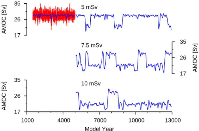
Fig. 1. Time series of the maximum of the North Atlantic Ocean meridional overturning (AMOC), calculated north of 30◦N and be-low 500-m water depth. Positive values indicate poleward fbe-low in the upper branch of the overturning cell. (Top) Unsmoothed an-nual values (red) from the unperturbed control experiment (prior to model year 5000). The corresponding output from a 101-year wide Hanning filter is overlain (blue). After model year 5000 a 5 mSv freshwater perturbation is applied in the Labrador Sea. The resulting AMOC time series (smoothed) oscillates between approx-imately 22 and 28 Sv. (Center) AMOC for a 7.5 mSv freshwater perturbation starting in model year 5000 (smoothed time series). (Bottom) As before but for a 10 mSv forcing.

et al., 2004). Therefore, disentangling these interglacial cli-mate fluctuations may also help to better understand glacial climate fluctuations.

2 Setup of the coupled climate-model experiments

To test the potential of the climate system to gener-ate low-frequency climgener-ate oscillations, we use the global atmosphere-ocean model ECBilt-CLIO, version 3 (more in-formation about the model including the source code is avail-able from www.knmi.nl/onderzk/CKO/ecbilt.html). This coupled model of intermediate complexity derives from the atmosphere model ECBilt (Opsteegh et al., 1998) and the ocean and sea-ice model CLIO (Goosse and Fichefet, 1999). The atmospheric component solves the quasi-geostrophic equations with T21 resolution (∼5.6◦) for three layers and uses simplified parameterizations for atmospheric thermody-namics. The model contains a full hydrological cycle. Vari-ability associated with large-scale weather patterns is explic-itly computed. The primitive-equation, free-surface ocean component has a horizontal resolution of 3◦and 20 levels in the vertical and uses a rotated subgrid in the North Atlantic Ocean to avoid the convergence of meridians near the north pole. It includes parameterizations for mixed-layer dynam-ics, downsloping currents and Gent-McWilliams (1990) pa-rameterization of subgrid-scale processes. The ocean model is coupled to a thermodynamic-dynamic sea-ice model with

viscous-plastic rheology. There is no local flux correction in ECBilt-CLIO. However, precipitation over the Atlantic and Arctic basins is reduced by 8.5% and 25%, respectively, and homogeneously redistributed over the North Pacific.

Beside a 5000-yr (year) long control run, simulating the modern (i.e., pre-industrial with respect to atmospheric greenhouse-gas concentration, orbital configuration, and land cover) climate, we conducted three experiments in which a perturbation of approximately 30, 45 and 60 cm/yr, respectively was continuously added to the precipitation field over the southern Labrador Sea. The resulting freshwa-ter forcings amount to 5, 7.5 and 10 mSv (milli-Sverdrup; 1 Sv=106m3/s), respectively, which is at least one order of magnitude below the values typically used in freshwater-hosing experiments to yield a complete shut-down of deep-water formation in the North Atlantic (Stouffer et al., 2006). The local perturbation was globally compensated to close the mass balance. The applied precipitation anomalies are of the same order of magnitude as the annually averaged precipita-tion over the Labrador Sea area which amounts to 43 cm/yr in the control run. All other boundary conditions in the sensitiv-ity experiments were kept the same as in the control run. For each sensitivity experiment, the model was integrated for an-other 8000 yr, starting from the final state of the control run as initial condition. All model results presented below are based on annual mean values.

3 Simulation results

In the unperturbed control simulation the strength of the AMOC varies between 20 and 35 Sv with a mean value of 28 Sv and a standard deviation of ∼2 Sv (Fig. 1, top). Spec-tral analysis reveals that the variability of the AMOC shows a slight tendency towards characteristic timescales of ap-proximately 12 and 200 years (not shown; see Goosse et al. (2003) for a discussion of the variability in ECBilt-CLIO). Since our main interest is in low-frequency variability, i.e., in timescales of at least a few hundred years, we turn to smoothed AMOC time series in the following. Smoothing was performed with a 101-year wide Hanning filter. For the unperturbed control experiment, the smoothed AMOC strength lies between 25 and 29 Sv (Fig. 1, top).

For the freshwater perturbation of 5 mSv the character of the modeled AMOC changes fundamentally. The forcing gives rise to a bi-modal AMOC distribution with values of approximately 28 and 22 Sv (Fig. 1, top). In the following these states of the AMOC will be referred to as “strong” and “weak” states. It is noteworthy that the AMOC oscil-lates between two states with positive AMOC values, that is, deep-water formation in the North Atlantic Ocean never ceases during the oscillations. Using an arbitrary threshold value of 25 Sv to separate weak and strong states, we find that the model spends 80% of the time in the strong state. Accordingly, the weak state can be viewed as a perturbation

a

b

c

d

Fig. 2. Mixed-layer depth and meridional overturning streamfunction in the Atlantic Ocean. (a) Mixed-layer depth [m] for the strong state, with deep mixing in the Labrador Sea and Nordic Seas. (b) Meridional overturning streamfunction [Sv] for the strong state. Positive values indicate clockwise rotation. (c, d) As a, b but for the weak state without deep-water formation in the Labrador Sea. All plots are based on annual mean values from the 7.5 mSv experiment, averaged over model years 8000–8050 (strong state) and 8900–8950 (weak state).

of the strong state, lasting between approximately 100 and 700 years.

If the freshwater forcing is increased to 7.5 mSv the princi-pal bi-modality of the AMOC is maintained (Fig. 1, center). However, with the increased magnitude of the forcing, the model stays only 33% of the time in the strong state. This suggests a tendency for remaining longer in the weak state as the freshwater forcing in the Labrador Sea increases. In this experiment, a total of six weak-to-strong transitions can be observed. The duration between subsequent transitions (in the order of their appearance) is approximately 540, 1360, 310, 2660, and 2220 years. Finally, by increasing the fresh-water perturbation to 10 mSv, the model resides in the strong state for only 14% of the time. Accordingly, the previously identified propensity of the model to stay in the weak state for an increased freshwater perturbation gains further support.

To better understand the origin of the AMOC variations we turn to changes in deep-water formation sites in the North Atlantic Ocean. For the strong state, mixed-layer depth points to two sites where deep mixing and, hence, deep-water formation takes places, namely the Nordic Seas and the Labrador Sea (Fig. 2a). The corresponding meridional over-turning streamfunction indicates that approximately 16 Sv of the newly formed deep water in the North Atlantic are ex-ported across 30◦S into the Southern Ocean (Fig. 2b). Be-low this layer, approximately 5 Sv of Antarctic Bottom Water

enter the Atlantic basin. Both mixed-layer depth and merid-ional overturning streamfunction are practically identical be-tween the strong state in the 7.5 mSv experiment (Fig. 2a, b) and the unperturbed control experiment (i.e., before model year 5000), which is therefore not shown. In contrast to the strong state, deep-mixing in the weak state is limited to the Nordic Seas (Fig. 2c), where the mixed-layer depth also in-creases (cf. Figs. 2a, c). Although the absence of deep-water formation in the Labrador Sea leads to a reduction in the maximum of the meridional overturning streamfunction by 6 Sv (Fig. 2b, d) the export to the Southern Ocean decreases by only 2 Sv to a value of 14 Sv. The changes in deep-water formation in the North Atlantic Ocean have no significant effect on the inflow of Antarctic Bottom Water which re-mains at 5 Sv. Mixed-layer depth and meridional overturn-ing streamfunction for the weak and strong states show only negligible differences between the different sensitivity exper-iments. Hence, we limit the presentation of results to those shown in Fig. 2.

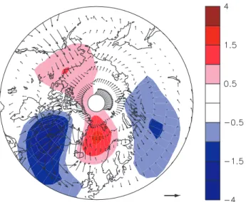
The cessation of deep-water formation in the Labrador Sea in the weak state causes a drop in surface-air temperature in this region by up to 3◦C (Fig. 3). At the same time, air temperature rises by up to 1.5◦C north of Iceland associated with an increase in oceanic heat transport by approximately 0.05 PW (not shown). This increased heat transport is due to the slightly enhanced deep-water formation in the Nordic

Fig. 3. Near-surface (2 m) air-temperature difference [◦C] between weak state and strong state in the northern hemisphere. Anomalies are based on annual mean values from the 7.5 mSv experiment, av-eraged over model years 8000–8050 (strong state) and 8900–8950 (weak state). Arrows indicate corresponding wind field anomalies at the 800 hPa level (length of scale arrow in lower right corner is 0.7 m/s).

Seas and a deepening of the Icelandic Low, which enhances the wind-driven northward transport of warm Atlantic water into the Nordic Seas. It should be noted that the zero line between positive and negative temperature anomalies runs through central Greenland as well as Scandinavia (Fig. 3). While the principal pattern of these temperature anomalies is rather stable during the course of the weak state, the actual extent of the anomalies may vary. For example, the warm anomaly may be restricted to Iceland and the area immedi-ately north of it but may not encompass mainland Scandi-navia as is the case depicted in Fig. 3 (not shown).

In summary, the coupled ocean-atmosphere model ex-hibits internal oscillations of the AMOC at multicentennial-to-millennial timescales upon weak and continuous freshwa-ter forcing in the Labrador Sea. The oscillations are charac-terized by a strong state with deep-water formation in both, the Nordic Seas and Labrador Sea and a weak state in which deep water forms only in the Nordic Seas. The minimum (22 Sv) and maximum (28 Sv) values of the AMOC during the oscillations are virtually independent of the magnitude of the freshwater perturbation.

4 Discussion

In order to disentangle the dynamics underlying the mod-eled AMOC oscillations one has to answer the following two questions: (i) why does deep-water formation in the Labrador Sea switch between on and off states? and (ii) what determines the timescale of the oscillations? In our analysis

17 24 31 5000 7000 9000 11000 13000 32.5 33.5 34.5 35.5 AMOC [Sv] Salinity [psu] Model Year LS DS

Fig. 4. Surface-salinity variations in the North Atlantic Ocean and meridional overturning in the 7.5 mSv experiment. (Top) Salinity immediately north of Denmark Strait (DS, red) and in the central Labrador Sea (LS, black). Salinities are averaged from the surface to 50 m depth. (Bottom) Meridional overturning (as in Fig. 1, cen-ter). All time series are smoothed by a 101-year wide Hanning filter.

of the model results we will set out from the first question before tackling the second.

4.1 Origin of the oscillations

Today, the deep-water formation areas in the Nordic Seas and Labrador Sea are linked through the subpolar gyre, which advects low-salinity surface water from the Arctic Ocean via the East and West Greenland Currents to the Labrador Sea (e.g. Tomczak and Godfrey, 2002). With regard to the model results, the key elements to note are: Firstly, the deep-water formation site in the Labrador Sea is located “downstream” of the deep-water formation site in the Nordic Seas. Sec-ondly, deep water forms in the Labrador Sea despite the ad-vection of low-salinity water from the “upstream” area. In other words, today the Nordic Seas exert a counteracting ef-fect on mixing in the Labrador Sea and, therefore, deep-water formation in that area.

This oceanographic situation is well captured in the model, which resolves the two deep-water formation sites in the North Atlantic Ocean (a condition not always met by coarse-resolution climate models) and advects low-salinity surface water through Denmark Strait into the Labrador Sea. Imme-diately north of Denmark Strait, near-surface salinity is ap-proximately 1.5 psu lower than in the central Labrador Sea, where deep mixing occurs. The same situation prevails dur-ing the strong state of the AMOC oscillations (Fig. 4).

A contrasting situation arises for the weak state, in which a halocline forms in the Labrador Sea that prevents deep mix-ing. Hence, freshwater entering the Labrador Sea as runoff or precipitation leads to the build-up of a low-salinity sur-face layer in the Labrador Sea, thus re-inforcing the

halo-cline. Compared to the strong state, near-surface salinity drops by 2 psu to 33 psu in the central Labrador Sea (Fig. 4). At the same time, an anomalous wind pattern (Fig. 3) pushes saline surface water into the Nordic Seas. Subsequent hor-izontal mixing within the Nordic Seas raises salinity in the Greenland Sea by approximately 0.8 psu. Accordingly, sur-face salinity north of Denmark Strait is now almost 1.3 psu

higher than in the central Labrador Sea (Fig. 4). Advection

of this relatively saline water into the Labrador Sea helps to erode the halocline, hence, to re-establish deep-water forma-tion in the Labrador Sea. It should be noted that density vari-ations of the surface-water masses are dominated by salin-ity variations since average surface temperature vary only little around their mean values of −0.3 and −0.6◦C in the Labrador Sea and Greenland Sea, respectively.

Although the amount of freshwater forcing that moves the model into the oscillating regime will most likely depend on the magnitude of the overturning in the Atlantic Ocean, we surmise that the existence of the oscillation depends less strongly on the overall strength of the AMOC than on the ex-istence of two localities for deep-water formation. Accord-ingly, we consider the relatively large value of the AMOC in the control experiment (cf. Sect. 3) only of minor importance with respect to the existence of the oscillations.

In summary, independently of the state of the AMOC (weak vs. strong), the “upstream” deep-water formation area in the Nordic Seas always tends to induce a change in the mode of operation of the “downstream” Labrador Sea. Thus the switching between the strong and weak states of the AMOC depends critically on the influence that the upstream density reservoir exerts on the downstream reservoir. The lack of AMOC oscillations in the control experiment indi-cates that the effect of the upstream reservoir for modern boundary conditions is insufficient to turn off the deep mix-ing in the Labrador Sea. Only when a small amount of fresh-water is added to the Labrador Sea, the model crosses a crit-ical threshold and the oscillations appear. In other words, a small positive freshwater anomaly is sufficient to raise the sensitivity of the Labrador Sea to a level allowing a strong re-sponse to the influx of low-density water from the upstream reservoir.

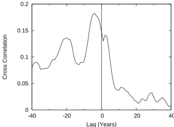
Cross-correlating maximum mixed-layer depth in the Labrador Sea with salinity (averaged over the top 50 m) im-mediately north of Denmark strait provides another way of looking at the proposed link between the two deep-water for-mation sites (Fig. 5). Salinity and mixed-layer depth show the expected positive correlation and the lead of salinity over mixed-layer depth of approximately 4 years is consistent with the postulated causal link.

Given this explanation of what controls the switching between active and inactive deep-water formation in the Labrador Sea, we can now turn to the second question re-garding the timing of these switches.

0 0.05 0.1 0.15 0.2 -40 -20 0 20 40 Cross Correlation Lag (Years)

Fig. 5. Cross correlation between maximum mixed-layer depth in the Labrador Sea and surface salinity (averaged over top 50 m) im-mediately north of Denmark Strait in the 7.5 mSv experiment. Max-imum of the correlation function at a lag of −4 years indicates that salinity anomalies precede mixed-layer anomalies by this amount of time. Analysis based on unsmoothed annual mean values.

4.2 Timescale of the oscillations

The duration between subsequent transitions varies widely from 310 to 2660 years in the 7.5 mSv experiment (Sect. 3; Fig. 1) and does not indicate a preferred timescale within this range. The average duration is approximately 1420 years and the standard deviation amounts to 1020 years. Hence, the to-tal range of values is almost completely covered by the in-terval of one standard deviation around the mean, supporting the notion that the durations are more or less uniformly dis-tributed (with only 5 durations at hand, no meaningful sta-tistical test of the distribution can be performed). The lack of a dominant timescale argues against a deterministic pro-cess controlling the timing of the AMOC oscillations and is easier to reconcile with a stochastic origin. (We use the term “stochastic” in a somewhat loose sense. In the model any “randomness” is generated by the interactions of determinis-tic processes which lead to high-frequency noise.)

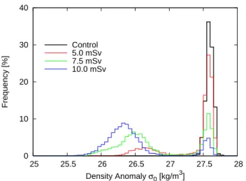
Starting from a state with active deep-water formation in the Labrador Sea, a randomly occurring negative density per-turbation of sufficient magnitude will reduce vertical mixing for example only in a single grid cell of the model. Due to the strong non-linear feedback associated with vertical mixing (e.g. Rahmstorf, 1995) a complete cessation of vertical mix-ing in the entire Labrador Sea can then result. For the control experiment this situation apparently never arises. One can assess the magnitude of the perturbations that occur in the control experiment from the surface density distribution in the Labrador Sea (Fig. 6). From this data, the probability that density falls below 27.35 kg/m3 is practically zero. A different situation arises when the Labrador Sea is perturbed by continuous freshwater input in the 5, 7.5 and 10 mSv

0 10 20 30 40 25 25.5 26 26.5 27 27.5 28 Frequency [%] Density Anomaly σ₀ [kg/m3] Control 5.0 mSv 7.5 mSv 10.0 mSv

Fig. 6. Histogram of surface density anomalies in the central Labrador Sea for all experiments. Anomalies (i.e., water density minus 1000 kg/m3) are averaged from the surface to 50 m depth.

The high-density mode at 27.6 kg/m3corresponds to active deep-water formation in the Labrador Sea (“strong” mode), whereas the low-density modes between 26.3 and 26.7 kg/m3 result when no deep mixing occurs (“weak” mode). Note that the control experi-ment (black) is characterized by a high-density mode only.

periments. While these perturbations by themselves are in-sufficient to shut down convection permanently, they make deep-water formation in the Labrador Sea more vulnerable to the randomly occurring negative density anomalies. It is the combined effect of the continuous freshwater forcing to-gether with random density anomalies that has the potential for bringing deep-water formation to a halt. Once convec-tion has ceased, lateral advecconvec-tion of water masses with rel-atively high densities, originating partly in the Nordic Seas (cf. Fig. 4), will start to erode the halocline that prevents deep-mixing in the Labrador Sea. As for the shutdown of deep-water formation it is, however, the superimposed effect of positive density anomalies occurring at random that ulti-mately re-initiate convection in the Labrador Sea.

Given the noise-induced transitions between the states with and without convection in the Labrador Sea, the change in the ratio of the duration of strong state to weak state of the AMOC oscillations (cf. Fig. 1) can be explained. Starting from a strong state, a larger value of the continuous fresh-water forcing brings the Labrador Sea closer to the point at which a random negative density anomaly can stop the deep mixing. Thus, the probability for a shutdown of convection in the Labrador Sea increases with increasing freshwater forc-ing (Fig. 6).

Once the system is in the weak mode, the likelihood for a large positive density anomaly determines how long this mode prevails. Since a larger freshwater forcing moves the Labrador Sea towards less dense surface waters, the proba-bility for a weak-to-strong transition decreases with increas-ing freshwater forcincreas-ing. This effect of the freshwater forcincreas-ing

can also be inferred from the histograms which show that the peak associated with the weak mode is shifted towards smaller densities for increasing values of the freshwater forc-ing (Fig. 6). In summary, the larger the freshwater forcforc-ing, the more likely is a transition from strong to weak modes and the more unlikely is a mode switch in the opposite direc-tion. The change in the likelihood for each state with varying freshwater forcing manifests itself in the shift in the ratio be-tween strong and weak modes discussed above (cf. Fig. 1). 4.3 Conceptual model of the oscillations

Probably the simplest model that captures the basic mech-anisms of the low-frequency oscillations consists of two prognostic variables, T and S, representing spatially aver-aged temperature and salinity of the upper (say, the topmost 200 m) Labrador Sea. Hydrographic conditions in the up-per Labrador Sea depend on the wind- and density-driven inflows from the subtropical Atlantic, the influx of subpolar water from the Greenland Sea (via the East Greenland Cur-rent through Denmark Strait) and surface fluxes. The deter-ministic governing equations for Labrador Sea temperature and salinity can therefore be formulated as

dS dt = 1 V h (q1+φ)S1+q2S2−(q1+q2+φ + P + P′)S i , (1) dT dt = 1 V h (q1+φ)T1+q2T2−(q1+q2+φ)T i +H, (2)

where V denotes the volume of the upper Labrador Sea (3×1014m3), q1 is the wind-driven volume flux from the

subtropical Atlantic, φ is the density-driven (overturning) volume flux from the subtropical Atlantic, q2 is the

vol-ume flux from the Greenland Sea, P denotes a basic sur-face freshwater flux into the Labrador Sea (78 mSv), P′ is a freshwater flux perturbation, H denotes the surface heat flux, and t is time. S1, T1and S2, T2 denote salinities and

temperatures of the inflowing subtropical and subpolar wa-ter masses, respectively. To keep the model as simple as possible, the wind-driven volume fluxes are assumed to be constant (q1=2 Sv, q2=2 Sv; after Fig. 10.50 in Dietrich et

al., 1975). Likewise, any temperature and salinity changes in the water masses originating from the subtropical Atlantic and the Greenland Sea are neglected (S1=35.3 psu, T1=8◦C, S2=34.6 psu, T2=1.5◦C). The overturning φ couples the pair

of differential equations through a linear dependence on the density difference between the Labrador Sea and the subtrop-ical Atlantic, i.e. φ=κ [α (T1–T)–β (S1–S)], where α and β

denote the thermal and haline expansion coefficients of sea-water (α=0.1 K−1, β=0.8 psu−1). The tuning parameter κ is set to 70 Sv. If φ becomes lower than zero, φ is set to zero (state of no overturning or “off” mode). For the sur-face heat flux H, a simple restoring term is used, i.e., H=(2–

is the relaxation time scale. This simple approach param-eterizes the damping of surface temperature anomalies by atmospheric heat advection and/or longwave radiation. An analogy for salinity does not exist since the atmosphere is insensitive to the presence of salinity anomalies.

In order to analyze the stability behavior of the simple de-terministic model, an equilibrium hysteresis with respect to surface freshwater forcing is calculated. It is well known that the competition between thermal and saline forcings of the overturning may result in multiple equilibria (Stommel, 1961). Plotting the overturning φ against the anomalous freshwater forcing P′reveals a regime of bi-stability for in-termediate forcing amplitudes (Fig. 7). With P′=0 Sv, for instance, one stable equilibrium (“off” mode) has zero over-turning and a Labrador Sea salinity of S∼=34.3 psu, while the other stable equilibrium (“on” mode) yields an overturn-ing of φ=10 Sv and a salinity of ∼35.0 psu. For very large positive/negative values of P′_{, only the “off”/“on” mode of}

Labrador Sea overturning provides a stable solution. Since the inflow of subpolar water (S2=34.6 psu) has a higher/lower

salinity than the Labrador Sea in the “off”/“on” mode, it will always counteract the current state of overturning in the Labrador Sea. To demonstrate this, we calculate another equilibrium hysteresis with q2set to zero (Fig. 7, red curve).

As a result of the missing northern inflow, the hysteresis loop widens, i.e., larger positive or negative freshwater perturba-tions P′are necessary to induce a transition from one mode to the other.

The simple model possesses no internal variability. In the bi-stable regime of ocean circulation, however, occasional state transitions can be introduced by a stochastic forcing component (cf. Cessi, 1994). We add a term σ ξ S0/V to

Eq. (1) to introduce a stochastic component in the salinity balance, where ξ represents Gaussian “quasi white noise” with zero mean and unit variance (a non-vanishing autocor-relation up to 3 days is introduced by the 3-days time step of the Euler forward scheme used to solve the differential equa-tions), σ measures the standard deviation of the stochastic forcing and S0 denotes a reference salinity (35 psu).

Set-ting σ =0.2 Sv and applying no additional freshwater flux (P′=0 Sv), we obtain numerous transitions from one mode to the other during a 50 000 year integration, resulting in multicentennial-to-millennial variations of the overturning circulation (Fig. 8). The mean residence time in a circula-tion mode before switching back to the other state (or the Kramers rate) and, hence, the timescale of the oscillations is given by the noise intensity (cf. Cessi, 1994). The stronger the noise, the larger is the probability for a flip into the other equilibrium, and the shorter is the mean residence time in one mode. Note, however, that the underlying bi-stability of the deterministic system may be completely masked if the am-plitude of the stochastic forcing is too strong (cf. Monahan, 2002; Stommel and Young, 1993). The value of σ =0.2 Sv was chosen such that the oscillations produced by the simple stochastic model are similar to the oscillations observed in

−60 −40 −20 0 20 0 2 4 6 8 10 12 14 16 18 Freshwater Input [mSv] Overturning [Sv]

All inflows included

No Greenland Sea inflow

Fig. 7. Equilibrium hysteresis loops (Labrador Sea overturning

φ vs. freshwater input P′) for the deterministic conceptual model with (black) and without (red) inflow from the Greenland Sea to the Labrador Sea. The hysteresis loops have been obtained by slowly varying the freshwater input into the Labrador Sea in the direction indicated by the arrows.

ECBilt-CLIO (given that the “off”/ “on” mode of the concep-tual model corresponds to the weak/strong mode in ECBilt-CLIO, where Labrador Sea convection is switched off/on). Moreover, the conceptual model captures the response of the 3-dimensional climate model to additional constant freshwa-ter inputs. With positive/negative constant perturbation, the system spends more time in the “off”/“on” mode (Fig. 8, left column; Fig. 9), since larger random perturbations are required to induce a transition to the “on”/“off” mode. In the absence of a subpolar water inflow from the Greenland Sea (q2=0 Sv) state transitions become unlikely (Fig. 8, right

column) due to the different stability behavior of the system associated with the wider hysteresis loop. In other words, the inflow from the Greenland Sea via Denmark Strait favors stochastic switches from one mode to the other.

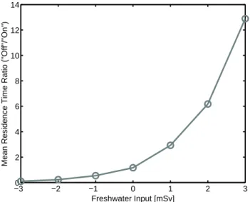
With Greenland Sea inflow a systematic relationship emerges between the mean residence-time ratio (i.e., the ra-tio between the mean residence times in the “off” mode and the “on” mode) and the constant freshwater perturbation P′ (Fig. 9). The higher the anomalous freshwater input into the Labrador Sea, the longer is the mean residence time in the “off” mode. Histograms of Labrador Sea density show, how-ever, that both modes are significantly populated for a cer-tain range of constant freshwater input P′ (Fig. 10). Over this P′-range, small freshwater inputs shift the frequency from the high- to the low-density mode of the probability density function – exactly as in ECBilt-CLIO (Fig. 6). For large freshwater inputs, the bi-modal structure of the proba-bility density vanishes (not shown). Note that the variance of the “off” mode distribution is larger than that of the “on”

0 10 20 30 40 50 26.8 27 27.2 27.4 27.6 27.8 −2 mSv 0 10 20 30 40 50 26.8 27 27.2 27.4 27.6 27.8 −2 mSv 0 10 20 30 40 50 26.8 27 27.2 27.4 27.6 27.8 +0 mSv Density [kg/m 3 ] 0 10 20 30 40 50 26.8 27 27.2 27.4 27.6 27.8 +0 mSv 0 10 20 30 40 50 26.8 27 27.2 27.4 27.6 27.8 +2 mSv kyr Density [kg/m 3 ] 0 10 20 30 40 50 26.8 27 27.2 27.4 27.6 27.8 +2 mSv kyr

All inflows included No Greenland Sea inflow

Density [kg/m

3 ]

Fig. 8. Typical time series of Labrador Sea density anomalies in the stochastically forced (σ =0.2 Sv) conceptual model with (black, left column) all inflows included and (red, right column) Greenland Sea inflow set to zero. From top to bottom, the additional constant freshwater influx P′increases from −2 mSv to +2 mSv.

mode, as it is in ECBilt-CLIO. This is due to a regulation of Labrador Sea density by the overturning circulation on short timescales which is only active in the “on” mode: if Labrador Sea density increases, the overturning and hence the inflow of warm, low-density subtropical water increases, counter-acting the initial density increase in the Labrador Sea. The conceptual model is able to capture this mechanism due to the inclusion of a variable Labrador Sea temperature (Eq. 2). In summary, the simple non-linear stochastic model re-produces the low-frequency oscillations observed in ECBilt-CLIO. It captures not only the occasional transitions from one equilibrium to the other, but also the variance of the fluc-tuations around each state. In doing so, it is capable to elu-cidate the physics behind the oscillations found in ECBilt-CLIO. These oscillations can be attributed to an underlying bi-stability in Labrador Sea convection and state transitions induced by noise. A slightly more complex approach for a conceptual model could have accounted for variations in Greenland Sea salinity variations. As shown in Fig. 4, Green-land Sea salinity slightly varies between the weak and strong mode in ECBilt-CLIO (substantial variations in subtropical salinities have not been found). An increase/decrease in

Greenland Sea salinity in the “off”/“on” mode would have a counteracting effect on the respective state of circulation. In other words, the equilibrium hysteresis would become nar-rower as compared to the case with fixed Greenland Sea salinity. This would favor state transitions under stochastic forcing, resulting in a higher frequency of the oscillations. A reduction in the noise intensity σ could compensate for this effect, leading to the same oscillations as those presented in Fig. 8. The conclusions drawn from our minimal model would be largely unaffected.

4.4 Comparison with oscillations found in other model ex-periments

The timescale of the oscillations in our experiments is sim-ilar to those resulting from so-called “deep-decoupling os-cillations” (Winton, 1993), which have been observed in 2-dimensional (e.g. Winton, 1993; Paul and Schulz, 2002) and 3-dimensional (Timmermann and Goosse, 2004) models of the ocean. However, the two types of oscillations have to be clearly distinguished. The oscillations described here are in-trinsically linked to the 3-dimensional flow field of the North

−30 −2 −1 0 1 2 3 2 4 6 8 10 12 14 Freshwater Input [mSv]

Mean Residence Time Ratio ("Off"/"On")

Fig. 9. Relation between the mean residence time ratio (i.e. the ratio between the mean residence times in the “off” mode and the “on” mode) and the constant freshwater input P′ in the stochastically forced (σ =0.2 Sv) conceptual model.

Atlantic Ocean, while deep-decoupling oscillations are asso-ciated with diffusive heat transport in the subsurface layer. Indeed, a crucial role of the freshwater transport through Denmark Strait in controlling the convection seesaw between the Labrador Sea and Nordic Seas has also been observed in a more comprehensive 3-dimensional climate model (Oka et al., 2006). However, the variability in this model oc-curs at interdecadal timescales and not at multicentennial-to-millennial timescales as seen in our model experiments.

Abrupt changes in the strength of the AMOC at millen-nial timescales were also found in an earlier version of the ECBilt-CLIO model (Goosse et al., 2002). The authors de-scribe a spontaneous weakening of the overturning strength that occurred twice within an approximately 10 000-year long experiment. Each event lasted for 100 to 250 years. Al-though the resulting time series bear some similarity with the results of our 5-mSv experiment, the underlying mechanisms are different. In the model version employed by Goosse et al. (2002) deep convection in the North Atlantic Ocean oc-curred only in the Nordic Seas and not in the Labrador Sea. In their model, the changes in deep-water production rate were associated with spontaneous shifts in convection depth and location within the Nordic Seas. While the underlying mechanism thus differs from our experiments, a commonal-ity exists in that the timings of the events occur by chance. 4.5 Relevance for past climate variations

Whether or not the oscillations described in this study did oc-cur in the past, can be tested by contrasting deep-water for-mation proxies from the Labrador Sea with proxies from the Nordic Seas. Indeed, a paleoceanographic reconstruction for

27 27.1 27.2 27.3 27.4 27.5 27.6 27.7 0 2 4 6 8 10 12 14 16 18 Density Anomaly [kg/m3] Frequency [%] −3 mSv −2 mSv −1 mSv +0 mSv +1 mSv +2 mSv +3 mSv

Fig. 10. Probability density functions of Labrador Sea density-anomalies in the stochastically forced (σ =0.2 Sv) conceptual model for different constant freshwater perturbations P′between −3 mSv and +3 mSv.

the Labrador Sea suggests changes in deep convection at mil-lennial timescales throughout the Holocene (Hillaire-Marcel et al., 2001). Although these authors interpret the record in terms of varying sea-ice export from the Arctic Ocean, the results are also compatible with the oscillations found in our model experiments. Paleoceanographic records from the Nordic Seas are also indicative of millennial-scale varia-tions during the Holocene (e.g. Andersson et al., 2003; Rise-brobakken et al., 2003). However, due to stratigraphic un-certainties, it is currently impossible to test the seesaw con-vection pattern predicted by the model using paleoclimatic data. We would like to stress, however, that the existing re-constructions are in harmony with our model results.

It has long been recognized that temperature reconstruc-tions from central Greenland show only little variability dur-ing the Holocene (specifically, if compared to the last glacial period; e.g. Grootes and Stuiver, 1997), while other regions in the North-Atlantic realm document considerable climate fluctuations (e.g. Mayewski et al., 2004). This observation is in line with our model experiments which suggest, based on the predicted surface-air temperature anomalies (Fig. 3), that central Greenland is rather insensitive to changes during interglacials. Larger temperature variations can be expected to be documented in southern Greenland (cf. Fig. 3), which is in agreement with paleoclimatic evidence from borehole records (Dahl-Jensen et al., 1998).

Based on temperature and precipitation proxies, it has been suggested that climate anomaly patterns at millennial timescales in the North-Atlantic region during the Holocene resemble the seesaw-pattern associated with the North At-lantic Oscillation (NAO; e.g. Nesje et al., 2001; Schulz and Paul, 2002). However, the millennial timescale of the

Holocene variations is difficult to reconcile with the dynam-ics underlying the NAO which favor variations at annual-to-decadal timescales (e.g. Hurrell et al., 2003). Moreover, Visbeck et al. (1998) showed that the oceanic response to atmospheric NAO forcing does not result in a seesaw-type temperature-anomaly pattern at timescales longer than some decades. Our model results indicate that the low-frequency oscillations associated with the on and off states of deep con-vection in the Labrador Sea give rise to a temperature see-saw between western Scandinavia and West Greenland that is akin to the seesaw associated with the NAO (e.g. Hur-rell et al., 2003). However, the underlying dynamics be-tween the modeled oscillations and the NAO differ funda-mentally, suggesting that it might be misleading to interpret climate anomaly patterns in terms of the dominant interan-nual modes of present-day climate variability across a wide range of timescales.

With respect to reconstructed climate variations during the Holocene, our results offer a potential mechanism to explain the observed low-frequency variability by an internal mech-anism. However, such an interpretation immediately leads to the question, which mechanism moves the system into the bi-stable regime (i.e., provides the continuous freshwa-ter forcing to the Labrador Sea). The simplest answer may be that the Holocene climate has been in this mode for most of the time and that the random nature and small amplitude of the oscillations simply hampered their coherent detection at a hemispheric scale. (In addition, the detection is impeded by stratigraphic uncertainties.) It may equally well be that the internal oscillations get phase-locked to external (e.g. so-lar) forcing at multicentennial timescales (Bond et al., 2001), thus providing an amplifier for the inferred solar forcing of Holocene climate change. The potential of this mechanism with respect to Holocene climate variability will be the sub-ject of a forthcoming study. Finally, we would like to point out that the temperature fluctuations associated with the os-cillations are much smaller than the variations associated with the glacial Dansgaard-Oeschger events (e.g. Voelker, 2002). Moreover, the temperature seesaw between Labrador Sea and Nordic Seas is not consistent with the overall cool-ing in the North-Atlantic region durcool-ing Dansgaard-Oeschger stadials (e.g. Voelker, 2002). Hence, while we think that the low-frequency oscillations are important with respect to in-terglacial climate variability, their role in generating glacial climate variability is probably small.

5 Summary and conclusions

Our model experiments suggest that interactions between the Nordic Seas and the Labrador Sea can result in oscil-lations of the overturning circulation of the Atlantic Ocean at multicentennial-to-millennial timescales. A continuous freshwater input into the Labrador Sea can push the large-scale ocean circulation into a bi-stable regime, which is

char-acterized by phases of active and inactive deep-water forma-tion in the Labrador Sea. In contrast, deep-water formaforma-tion in the Nordic Seas is active during all phases of the oscil-lations. The near-surface flow through Denmark Strait cou-ples the two deep-water formation regions through the ad-vection of density anomalies which always tend to coun-teract the deep-water formation mode of the Labrador Sea. The actual timing of the transitions between the circula-tion states occurs randomly. The oscillacircula-tions constitute a 3-dimensional phenomenon and have to be clearly distin-guished from low-frequency oscillations seen previously in 2-dimensional models of the ocean. Experiments with other 3-dimensional climate models, specifically more comprehen-sive models, should be carried out to test the robustness of the mechanism that gives rise to the low-frequency AMOC oscillations in our climate model of intermediate complexity and their potential interactions with future climate change.

Acknowledgements. We thank P. Herrmann for developing most

useful netCDF routines for ECBilt-CLIO and H. Goosse for his continued improvement of the model. We are grateful to the two referees for their comments and recommendations which helped us greatly to improve the text. This work was supported by the Deutsche Forschungsgemeinschaft through DFG Research Center “Ocean Margins”. This is RCOM publication 0465.

Edited by: P. Wang

References

Andersson, C., Risebrobakken, B., Jansen, E., and Dahl, S. O.: Late Holocene surface ocean conditions of the Nor-wegian Sea (Vøring Plateau), Paleoceanography, 18, 1044, doi:10.1029/2001PA000654, 2003.

Bianchi, G. G. and McCave, I. N.: Holocene periodicity in North Atlantic climate and deep-ocean flow south of Iceland, Nature, 397, 515–517, 1999.

Bond, G., Kromer, B., Beer, J., Muscheler, R., Evans, M. N., Show-ers, W., Hoffmann, S., Lotti-Bond, R., Hajdas, I., and Bonani, G.: Persistent solar influence on North Atlantic climate during the Holocene, Science, 294, 2130–2136, 2001.

Bond, G., Showers, W., Cheseby, M., Lotti, R., Almasi, P., de-Menocal, P., Priore, P., Cullen, H., Hajdas, I., and Bonani, G.: A pervasive millennial-scale cycle in North Atlantic Holocene and glacial climates, Science, 278, 1257–1266, 1997.

Cessi, P.: A simple box model of stochastically forced thermohaline flow, J. Phys. Oceanogr., 24, 1911–1920, 1994.

Chapman, M. R. and Shackleton, N. J.: Evidence of 550-year and 1000-year cyclicities in North Atlantic circulation patterns dur-ing the Holocene, The Holocene, 10, 287–291, 2000.

Dahl-Jensen, D., Mosegaard, K., Gundestrup, N., Clow, G. D., Johnsen, S. J., Hansen, A. W., and Balling, N.: Past temperatures directly from the Greenland ice sheet, Science, 282, 268–271, 1998.

Dietrich, G., Kalle, K., Krauss, W., and Siedler, G.: Allgemeine Meereskunde, Gebr. Borntraeger, Berlin, 593, 1975.

Gent, P. R. and McWilliams, J. C.: Isopycnal mixing in ocean cir-culation models, J. Phys. Oceanogr., 20, 150–155, 1990.

Goosse, H. and Fichefet, T.: Importance of ice-ocean interactions for the global ocean circulation: A model study, J. Geophys. Res., C104, 23 337–23 355, 1999.

Goosse, H., Renssen, H., Selten, F. M., Haarsma, R. J., and Op-steegh, J. D.: Potential causes of abrupt climate events: A nu-merical study with a three-dimensional climate model, Geophys. Res. Lett., 29, 1860, doi:10.1029/2002GL014993, 2002. Goosse, H., Selten, F. M., Haarsma, R. J., and Opsteegh, J. D.:

Large sea-ice volume anomalies simulated in a coupled climate model, Clim. Dyn., 20, 523–536, 2003.

Grootes, P. M. and Stuiver, M.: Oxygen 18/16 variability in Green-land snow and ice with 10−3- to 105-year time resolution, J. Geo-phys. Res., C102, 26 455–26 470, 1997.

Hall, A. and Stouffer, R. J.: An abrupt climate event in a coupled ocean-atmosphere simulation without external forcing, Nature, 409, 171–174, 2001.

Hall, I. R., Bianchi, G. G., and Evans, J. R.: Centennial to millennial scale Holocene climate-deep water linkage in the North Atlantic, Quatern. Sci. Rev., 23, 1529–1536, 2004.

Hillaire-Marcel, C., de Vernal, A., Bilodeau, G., and Weaver, A. J.: Absence of deep-water formation in the Labrador Sea during the last interglacial period, Nature, 410, 1073–1077, 2001.

Hurrell, J. W., Kushnir, Y., Ottersen, G., and Visbeck, M.: An Overview of the North Atlantic Oscillation, in: The North At-lantic Oscillation, edited by: Hurrell, J. W., Kushnir, Y., Ottersen, G., and Visbeck, M., Washington D.C., 1–35, 2003.

Knutti, R. and Stocker, T. F.: Limited predictability of future ther-mohaline circulation close to an instability threshold, J. Clim., 15, 179–186, 2002.

Mayewski, P. A., Rohling, E. E., Stager, J. C., Karl´en, W., Maasch, K. A., Meeker, L. D., Meyerson, E. A., Gasse, F., van Kreveld, S., Holmgren, K., Lee-Thorp, J., Rosqvist, G., Rack, F., Staub-wasser, M., Schneider, R. R., and Steig, E. J.: Holocene climate variability, Quatern. Res., 62, 243–255, 2004.

Monahan, A. H.: Stabilisation of climate regimes by noise in a sim-ple model of the thermohaline circulation, J. Phys. Oceanogr., 32, 2072–2085, 2002.

Nesje, A., Matthews, J. A., Dahl, S. O., Berrisford, M. S., and Andersson, C.: Holocene glacier fluctuations of Flatebreen and winter-precipitation changes in the Jostedalsbreen region, west-ern Norway, based on glaciolacustrine sediment records, The Holocene, 11, 267–280, 2001.

O’Brien, S. R., Mayewski, P. A., Meeker, L. D., Meese, D. A., Twickler, M. S., and Whitlow, S. I.: Complexity of Holocene cli-mate as reconstructed from a Greenland ice core, Science, 270, 1962–1964, 1995.

Oka, A., Hasumi, H., Okada, N., Sakamoto, T., and Suzuki, T.: Deep convection seesaw controlled by freshwater export through the Denmark Strait, Ocean Modell., 15, 157–176, 2006. Oppo, D. W., McManus, J. F., and Cullen, J. L.: Deepwater

vari-ability in the Holocene epoch, Nature, 422, 277–278, 2003. Opsteegh, J. D., Haarsma, R. J., Selten, F. M., and Kattenberg, A.:

ECBILT: a dynamic alternative to mixed boundary conditions in ocean models, Tellus, 50A, 348–367, 1998.

Paul, A. and Schulz, M.: Holocene climate variability on centennial-to-millennial time scales: 2. Internal feedbacks and external forcings as possible causes, in: Climate development and history of the North Atlantic Realm, edited by: Wefer, G., Berger, W. H., Behre, K.-E., and Jansen, E., Springer Verlag, Berlin, pp. 55–73, 2002.

Rahmstorf, S.: Bifurcations of the Atlantic thermohaline circulation in response to changes in the hydrological cycle, Nature, 378, 145–149, 1995.

Risebrobakken, B., Jansen, E., Andersson, C., Mjelde, E., and Hevrøy, K.: A high-resolution study of Holocene paleoclimatic and paleoceanographic changes in the Nordic Seas, Paleoceanog-raphy, 18, 1017, doi:10.1029/2002PA000764, 2003.

Sarnthein, M., van Kreveld, S., Erlenkeuser, H., Grootes, P., Kucera, M., Pflaumann, U., and Schulz, M.: Centennial-to-millennial-scale periodicities of Holocene climate and sediment injections off the western Barents shelf, 75◦N, Boreas, 32, 447–461, 2003. Schulz, M. and Paul, A.: Holocene climate variability on centennial-to-millennial time scales: 1. Climate records from the North-Atlantic realm, in: Climate development and history of the North Atlantic Realm, edited by: Wefer, G., Berger, W. H., Behre, K.-E., and Jansen, E., Springer Verlag, Berlin, pp. 41–54, 2002.

Schulz, M., Paul, A., and Timmermann, A.: Glacial-Interglacial Contrast in Climate Variability at Centennial-to-Millennial Timescales: Observations and Conceptual Model, Quatern. Sci. Rev., 23, 2219–2230, 2004.

Stommel, H.: Thermohaline convection with two stable regimes of flow, Tellus, 13, 224–228, 1961.

Stommel, H. and Young, W.: The average T-S relation of a stochastically-forced box model, J. Phys. Oceanogr., 23, 151– 158, 1993.

Stouffer, R. J., Yin, J., Gregory, J. M., Dixon, K. W., Spelman, M. J., Hurlin, W., Weaver, A. J., Eby, M., Flato, G. M., Hasumi, H., Hu, A., Jungclaus, J. H., Kamenkovich, I. V., Levermann, A., Montoya, M., Murakami, S., Nawrath, S., Oka, A., Peltier, W. R., Robitaille, D. Y., Sokolov, A., Vettoretti, G., and Weber, S. L.: Investigating the causes of the response of the thermohaline circulation to past and future climate changes, J. Clim., 19, 1365– 1387, 2006.

Timmermann, A. and Goosse, H.: Is the wind stress forcing essen-tial for the meridional overturning circulation?, Geophys. Res. Lett., 31, L04303, 10.1029/2003GL018777, 2004.

Tomczak, M. and Godfrey, J. S.: Regional oceanography: an intro-duction, pp. 391, 2002.

Visbeck, M., Cullen, H., Krahmann, G., and Naik, N.: An ocean model’s response to North Atlantic Oscillation-like wind forcing, Geophys. Res. Lett., 25, 4521–4524, 1998.

Voelker, A. H. L. and participants: Global distribution of centennial-scale records for Marine Isotope Stage (MIS) 3: a database, Quatern. Sci. Rev., 21, 1185–1212, 2002.

Winton, M.: Deep decoupling oscillations of the oceanic thermoha-line circulation, in: Ice in the climate system, edited by: Peltier, W. R., Springer Verlag, Berlin, pp. 417–432, 1993.