HAL Id: hal-00297555
https://hal.archives-ouvertes.fr/hal-00297555
Submitted on 15 May 2006
HAL is a multi-disciplinary open access
archive for the deposit and dissemination of
sci-entific research documents, whether they are
pub-lished or not. The documents may come from
teaching and research institutions in France or
abroad, or from public or private research centers.
L’archive ouverte pluridisciplinaire HAL, est
destinée au dépôt et à la diffusion de documents
scientifiques de niveau recherche, publiés ou non,
émanant des établissements d’enseignement et de
recherche français ou étrangers, des laboratoires
publics ou privés.
moisture?
N. Altimir, P. Kolari, J.-P. Tuovinen, T. Vesala, J. Bäck, T. Suni, M.
Kulmala, P. Hari
To cite this version:
N. Altimir, P. Kolari, J.-P. Tuovinen, T. Vesala, J. Bäck, et al.. Foliage surface ozone deposition:
a role for surface moisture?. Biogeosciences, European Geosciences Union, 2006, 3 (2), pp.209-228.
�hal-00297555�
www.biogeosciences.net/3/209/2006/ © Author(s) 2006. This work is licensed under a Creative Commons License.
Biogeosciences
Foliage surface ozone deposition: a role for surface moisture?
N. Altimir1,2, P. Kolari1, J.-P. Tuovinen3, T. Vesala2, J. B¨ack1, T. Suni2,4, M. Kulmala2, and P. Hari1 1Department of Forest Ecology, University of Helsinki, P.O. Box 27, FI-00014 Helsinki, Finland
2Department of Physical Sciences, University of Helsinki, P.O. Box 68, FI-00014 Helsinki, Finland
3Finnish Meteorological Institute, Climate and Global Change Research, P.O Box 503 FI-00101 Helsinki, Finland 4Land Air Interactions, CSIRO Marine and Atmospheric Research, Canberra,Australia
Received: 26 September 2005 – Published in Biogeosciences Discuss.: 22 November 2005 Revised: 7 March 2006 – Accepted: 23 March 2006 – Published: 15 May 2006
Abstract. This paper addresses the potential role of
sur-face wetness in ozone deposition to plant foliage. We stud-ied Scots pine foliage in field conditions at the SMEARII field measurement station in Finland. We used a combina-tion of data from flux measurement at the shoot (enclosure) and canopy scale (eddy covariance), information from fo-liage surface wetness sensors, and a broad array of ancillary measurements such as radiation, precipitation, temperature, and relative humidity. Environmental conditions were de-fined as moist during rain or high relative humidity and dur-ing the subsequent twelve hours from such events, circum-stances that were frequent at this boreal site. From the mea-sured fluxes we estimated the ozone conductance using it as the expression of the strength of ozone removal surface sink or total deposition. Further, we estimated the stomatal con-tribution and the remaining deposition was interpreted and analysed as the non-stomatal sink.
The combined time series of measurements showed that both shoot and canopy-scale ozone total deposition were en-hanced when moist conditions occurred. On average, the es-timated stomatal deposition accounted for half of the mea-sured removal at the shoot scale and one third at the canopy scale. However, during dry conditions the estimated stomatal uptake predicted the behaviour of the measured deposition, but during moist conditions there was disagreement. The es-timated non-stomatal sink was analysed against several envi-ronmental factors and the clearest connection was found with ambient relative humidity. The relationship disappeared un-der 70% relative humidity, a threshold that coincides with the value at which surface moisture gathers at the foliage surface according to the leaf surface wetness measurements. This suggests the non-stomatal ozone sink on the foliage to be modulated by the surface films. We attempted to extract such potential modulation with the estimated film formation via Correspondence to: N. Altimir
the theoretical expression of adsorption. Whereas this pro-cedure could predict the behaviour of the non-stomatal sink, it implied a chemical sink that was not accountable as sim-ple ozone decomposition. We discuss the existence of other mechanisms whose relevance in the removal of ozone needs to be clarified, in particular: a significant nocturnal stomatal aperture neglected in the estimations, and a potentially large chemical sink offered by reactive biogenic organic volatile compounds.
1 Introduction
Ozone (O3) is the main precursor of the important
hy-droxyl radical (OH), which governs the oxidative properties and self-cleansing mechanisms of the troposphere (Monks, 2005). Current tropospheric O3concentrations are
consid-ered a toxic threat to vegetation (Ashmore, 2005), and the en-suing injuries have been related to the uptake of O3through
the stomatal pores and oxidative effects damaging the inter-nal leaf tissue (Sandermann, 1996). It is considered more ap-propriate to establish cause-effect relationships based on the amount of O3 going into the foliage instead of the amount
of O3 present in the air (Ashmore et al., 2004). The
con-sequences for the plant are vastly different depending on whether the O3is removed by reactions inside the mesophyll
or outside at the foliage surface. Thus, it is relevant to be able to estimate not only the total amount of O3 deposited
onto a canopy but also the partition of the deposition fluxes, that is, where in the canopy and with what parts of it the O3
molecules ultimately react.
The flux of ozone towards a plant canopy is governed by the turbulent properties of the air flow around and within the canopy, the transfer at the diffusive boundary layer, and the properties of the sinks by which ozone is ultimately removed and/or deposited. The sink strength is determined by the combined effect of all removal pathways for ozone, which
include the stomatal uptake and the removal at the various canopy and forest surfaces.
To generate the flux of O3into a plant canopy, two kinds
of basic processes take place: chemical reactions and mass transport. O3 is a reactive molecule that readily oxidises a
variety of compounds, whether in gas-phase or in homoge-neous or heterogehomoge-neous reactions. Transport phenomena act by controlling the access of O3to the potential reaction
part-ners/sites. Turbulent transport facilitates such access through canopy-scale mixing, whereas molecular diffusion is less ef-ficient but controls the transport at smaller scales, e.g. close to surfaces. There is no known biological use to the flux of O3, but plant activity influences the flux of O3 through its
effect on the above-mentioned two basic processes.
The biological action in the process of ozone deposition is introduced most commonly through a description of stomatal behaviour based on measurements or estimations of transpi-ration (Baldocchi et al., 1987; Meyers et al., 1998; Simpson et al., 2003), which predict the dynamics of stomatal aperture to govern the deposition during the active seasons and ex-plain most of the daily and annual pattern. However, taking into account turbulent and diffusive transport , the stomatal uptake is not sufficient to predict the magnitude of the canopy sink. The so-called non-stomatal sinks have been invoked to explain the disagreement. The contribution of non-stomatal sinks to the total removal at the canopy scale can be on the order of 50% to 70% as reported from canopy scale mea-surements, This has been studied for a variety of ecosystems such as forests of Sitka spruce (Coe et al., 1995), spruce-fir (Zeller and Nikolov, 2000), or ponderosa pine (Kurpius and Goldstein, 2003), as well as low vegetation such as moor-land (Fowler et al., 2001), barley field (Gerosa et al., 2004), and at a miscellaneous Mediterranean sites (Cieslik, 2004). Measurements at the shoot scale have also revealed levels of deposition that exceed the prediction by stomatal uptake such as the measurements on Scots pine (Rond´on et al., 1993; Altimir et al., 2004) or laboratory measurements on poplar (van Hove et al., 1999). Non-stomatal deposition, particu-larly that involving external plant surfaces, is a major un-known in present understanding of biosphere-atmosphere gas exchange (Erisman et al., 2005; Wesely and Hicks, 2000).
This somewhat generic term of non-stomatal deposition compiles several processes that generally refer to gas-phase and/or heterogeneous chemical sinks inside and above the canopy. The relevance of various gas-phase reactions where ozone is involved has been discussed. The nitrogen oxides emitted from the soil may result in a significant consump-tion of O3(Duyzer et al., 1983; Pilegaard, 2001).
Quench-ing of organic volatiles in the atmosphere may also play a role (Kurpius and Goldstein, 2003, Goldstein et al., 2004; Mikkelsen et al., 2000, 2004), including reactions leading to aerosol formation (Bonn and Moortgat, 2003). The inten-sity of these reactions and their relevance as O3 sinks
de-pends on the presence and relative abundance of the various above-mentioned reactants. As to the foliage surfaces, it has
been argued that they can sustain ozone removal in several ways. Rond´on et al. (1993) and Coe et al. (1995) speculated on the possibility of photochemical reactions mediated by the foliage surface, based on the correlation of ozone depo-sition with temperature and solar radiation. Similar results were reported in Fowler et al. (2001), who also proposed that the non-stomatal flux could represent thermal decomposition of ozone at the surfaces. Several works have discussed the effect of wetness on the plant surfaces; for a summary on related studies see Massman (2004). There is a number of works that report either dew, rain, or high humidity increas-ing O3deposition as in the canopy measurements over
decid-uous and mixed forest in Finkelstein et al. (2000), the decidu-ous forest in Fuentes et al. (1992), the pine forest in Lamaud et al. (2002), as well as in the mixed and deciduous forests and fields of corn, soybean, and pasture studied in Zhang et al. (2002) and the field chamber measurements on Scots pine in Altimir et al. (2004). Variability in the reported ef-fects exists, whereas dew seemed to enhance O3deposition
to a grapevine field (Grantz et al., 1995) the effect was the contrary for a cotton field (Grantz et al., 1997) and Fuentes et al. (1994) report enhancement in maple but not in poplar leaves.
Sumner et al. (2004) showed the presence of water on sur-faces to be ubiquitous and discussed the need to address the implications for heterogeneous atmospheric chemistry. Sur-faces can hold a variable amount of wetness as a result of dew formation, rain, or ambient moisture. Dew and rain are held on the surface as droplets of liquid water (e.g. Brewer and Smith 1997); in addition, the waxy hydrophobic epicu-ticular surfaces can hold water monolayers, forming films or clusters that grow depending on the surrounding air humidity. The formation, growth and fate of water films on organic sur-faces depend on the chemical composition and corrugation degree of the surface (Rudich et al., 2000). The existence of water films on foliage surfaces and its influence on the deposition of gases has been extensively proposed in many studies (Burkhardt and Eiden, 1994; Burkhardt et al., 1999; Eiden et al., 1994; Kerstiens et al., 1992; Klemm et al., 2002; van Hove et al., 1989, 1996; Flechard et al., 1999; Sutton et al., 1998).
Measurements of O3fluxes close to the foliage are
espe-cially suitable to determine the relevance, or existence, of the mentioned O3 removal processes for which the foliage
surfaces might have a central role such as, in addition to the stomatal uptake, scavenging reactions mediated at the foliage surface and possibly controlled by several environmental fac-tors. The environmental drivers are connected to each other – e.g. temperature and relative humidity (RH )- and to the general daily course of environmental variables, including the existence of turbulence and the control of stomatal ac-tion. So, it may appear complex to address the relevance of one factor over the rest as to the control of the mechanism generating the deposition sink. The shoot enclosure provides a constrained approach that facilitates the examination and
together with a direct measure of the surface moisture it is possible to isolate the effects of surface moisture and tem-perature.
We analyse the dependence of ozone flux to foliage on environmental and biological factors aiming to identify the main removal processes, with special reference to the role of stomatal uptake and surface wetness. We used a combination of data from flux measurements on Scots pine foliage at the shoot (enclosure) and canopy scale (eddy covariance) and in-formation from foliage surface wetness sensors. We proceed in the following steps: a) we look at the patterns of deposi-tion, environmental variables and the relation between them b) we calculate and analyse the non-stomatal contribution c) we examine how moisture modulates the sink at the foliage surface and discuss alternative mechanisms.
2 Methods
2.1 Site
The measuring site is a Scots pine stand at the SMEAR II station in Hyyti¨al¨a, Southern Finland (61◦510N, 24◦170E, 180 m a.s.l.); for a general description of the station and the stand see Vesala et al. (1998). The stand was partly thinned between January and March 2002 to achieve a stem density of 800–1100 stems per ha and a reduction of 25% of the biomass. The resulting all-sided leaf area index (LAI) in the thinned areas was 6 and remained 8 in the unthinned portion of the stand.
The main part of the data was collected during 2002 and 2003, during which measurements of canopy fluxes and an-cillary meteorological measurements were running continu-ously. Shoot chambers were installed all-year around but for these two years data on O3 shoot fluxes was available only
from March to September.
Year 2002 was slightly atypical with the January-August period warmer than average and a quick change in September into a most cold winter. During 2003 the weather was some-what more typical although July was simultaneously warmer and more humid than normal and the late summer and au-tumn were very dry until October.
We differentiated between data measured under contrast-ing ambient conditions: dry/wet and day/night. We defined dry conditions as those above zero temperatures when there was no rain and it had been at least 12 h with RH lower than 70%. Otherwise, conditions were wet during rain, or if RH >70%, or if there had been such conditions within the previous 12 h. We defined nighttime as those times for which the measured photosynthetically active radiation PAR was less than 10 µmol m−2s−1. Note that boreal nights are comparatively short during summer and long during winter.
At this boreal forest site the efflux of nitrogen oxides from the forest floor is close to zero (<0.1 ngN m−2h−1)(Pihlatie
et al., 2003) and therefore the potential O3sink generated by
soil NO emissions could be ignored.
2.2 Moisture-related and other measurements
General meteorological measurements were available during the study period. Many variables are monitored at SMEARII, from which we detail the most relevant to this study. Unless otherwise stated, all sensors were placed above the canopy top. PAR was measured with a quantum sensor LI-190SZ (LiCor, USA). Ambient RH was calculated from the mea-sured dew point temperature (chilled mirror sensor, M4 Dew point monitor, General Eastern USA) and air temperature was measured with PT-100 sensors. Rain intensity was recorded in mm from a precipitation meter ARG-100 tip-ping bucket counter (Vector Instruments, UK) placed on a canopy clearing. Rain occurrence was measured by a DRD 11-A Rain Detector (Vaisala, Finland), which is based on droplet detection. The sensor is on a 30◦plane and is slightly heated to avoid water accumulation or condensation on the surface. This precludes fog detection, but melts the snow and allows snow detection. Fog occurrence was recorded ac-cording to visual assessment but because this is done at the same hour regardless of the season the records cannot regis-ter early morning fogs during summer.
Additionally, we arranged campaign-wise recordings of needle surface wetness (SW), which was measured by means of clip-type sensors (Burkhardt and Gerchau, 1994) clasped onto the surface of pine needles. The electrical resistance, or impedance, between the sensor’s electrodes was measured in order to detect the changes produced by the presence of wet-ness or moisture between them. A sensor consisted of two electrodes that aligned on both sides of the foliage length-wise so that the only plane where moisture could build up was the foliage surface. The conductivity of the tissue itself was not considered relevant because it is small compared to the surface wetness; also, the systems run on AC to avoid po-larising the tissues. Several of these sensors were attached to living needles in the canopy (9) and inside the gas-exchange chambers (1 per chamber) during 2002 and 2003, each of them clasped to 2–3 needles pairs. All sensors were in-spected regularly and the sensors in the canopy were changed to new needles every 4–5 weeks to avoid measuring damaged foliage, a situation that would ensue in the long run.
A completely wet surface e.g. under sustained rain- typi-cally produced a signal few hundred-fold that of a relatively non-wetted surface. This was the response used in previous studies using these sensors in canopies (Klemm and Man-gold, 2001; Klemm et al., 2002). The sensors were also sen-sitive to changes in surface moisture that come along with changes in ambient RH (Eiden et al., 1994). We were in-terested in this range of the SW sensor detection not only because precipitation is excluded from the foliage inside the chambers but also for the general interest of surface moisture of foliage in absence of liquid droplets. But the signal thus
produced was comparatively smaller and closer in magnitude to existing measuring noise and/or disturbances. In this con-text, we improved the data quality by correcting the influence of temperature on the SW sensor signal. The temperature de-pendence of a metallic electrical resistor is linear and can be predicted from metal-specific parameters and reference val-ues. However, we favoured a daily estimation of the linear dependence to allow for all possible temperature effects of the system, not only the resistor, to be taken into account. To such effect, we used the signal of an empty sensor to esti-mate a daily intercept and slope of signal versus temperature. The raw signal from any other sensor was then modified by subtracting the temperature-related signal.
2.3 Flux measurements
2.3.1 Shoot-scale fluxes
Shoot-scale fluxes were measured by a gas-exchange enclo-sure technique. The general performance of the chambers has been evaluated in Hari et al. (1999) with respect to CO2,
in Kolari et al. (2004) with respect to water and in Altimir et al. (2002, 2004) and Kulmala et al. (1999) with respect to O3. We measured on shoots from the top of the canopy;
they were installed inside the chamber into a horizontal posi-tion, debudded to prevent new growth, and the needles gently bent to form a plane. We also measured an empty equivalent chamber. The chambers remained open most of the time but closed intermittently (50–100 times per day) for one minute. From the change of gas concentration inside the chamber during the closure, we calculated the flux generated by the shoot by solving the mass balance equation. In case of O3: V · dC (t)
dt =q · (Ca−C(t)) − V · K · C(t) − A · gT ,O3·C(t) (1)
where the left-hand term is the time derivative of O3mass
inside the chamber, and the right-hand terms are the O3mass
flux produced by the sampling towards the gas analysers, the chamber walls, and the shoot, respectively. V (m3)is the internal volume of the enclosure, q (m3s−1)is the air flow rate through the chamber generated by the gas sampling, Ca
(gO3m−3)is ambient O3concentration, K (s−1)is rate
con-stant of O3loss to the chamber walls, A (m2)is the shoot
all-sided needle area and gT ,O3(m s
−1)is total shoot
conduc-tance. K was fitted on measurements from an empty cham-ber (omitting A·gT ,O3·C(t)) and its value was used when
fit-ting gT ,O3 to measurements with a shoot. In both cases, the
fit was performed to all the points during the chamber clo-sure.
In case of CO2and water vapour:
V · dC(t )
dt =q · (Ca−C(t )) − A · F (2)
where F is the net flux of CO2or water vapour (g m−2s−1),
which is obtained by a linear fit to the initial third of the
chamber closure. At high relative humidities (RH >70%) the amount of water adsorbed on the chamber walls increased steeply and disturbed the water vapour flux measurements, therefore, H2O fluxes measured in those conditions are not
reliable. At lower humidity, measured fluxes were corrected for the chamber wall effect according to Kolari et al. (2004). 2.3.2 Canopy-scale fluxes
Canopy fluxes were measured by the eddy covariance (EC) micrometeorological technique. O3fluxes were measured at
a height of at 22 m, which is 8 m above of the canopy, on a tower equipped with a fast-response acoustic anemometer and a fast response chemi-luminescence O3analyser.
Simul-taneous CO2 and water vapour fluxes were available from
the same tower. EC data also provided the parameter input needed for the flux analysis such as the intensity of turbu-lence or friction velocity (u∗) (cf. A.1). The details on set-ups
and the processing of the data have been presented elsewhere (Rannik, 1998; Buzorious et al., 1998; Keronen et al., 2003; Suni et al., 2003).
Nigthtime O3flux data was screened so that only
measure-ments during sufficient turbulence were accepted (as repre-sented by u∗>0.2 m s−1). On this basis, 16% of the
noc-turnal data was rejected (9% of the day time data contained u∗<0.2 m s−1).
The thinning did not introduce any dramatic changes in the behaviour of the measured canopy fluxes, neither there was a detectable difference in the fluxes from thinned and unthinned portions (Vesala et al., 2005). We make here no separation between these areas. We know from previous footprint analysis that under all conditions the contribution of the thinned area to the measured fluxes is highest when wind direction is 60–180◦, which represents only 26% of the measured data (Vesala et al., 2005). Most of the time the measured flux is representing both areas.
2.4 Flux analysis and surface conductances
The O3fluxes thus obtained are taken as a measure of the net
flux, or deposition, over the shoot and forest stand surfaces. The mechanisms generating the flux are analysed from the values of the concentration-normalised flux, which is related to the total ozone surface conductance that reflects the over-all proportionality constant of the scavenging processes, as follows:
In case of the shoot-scale measurements, the flux is in principle produced by the diffusional transport through the boundary layer and into the stomatal apertures, and the ensu-ing scavengensu-ing reactions at the inner and outer surfaces. The viscous boundary layer on the needle surfaces is kept at a constant value due to the ventilation inside the chambers, so it does not contribute to the pattern in the measured flux. The measured O3flux, thus, reflects changes in the stomatal
the surface is negligible, the net removal holds a first-order relation with O3 concentration and we define gT ,O3 (as in
Eq. 1) as the overall proportionality constant. It can also be defined as a concentration-normalised flux but we refer to it as the total shoot O3conductance. Parameter gT ,O3 can be
further decomposed:
gT ,O3 =gsto,O3+gnonsto,O3 (3)
where gsto,O3 is the part controlled by the stomatal action
(see below for its estimation) and gnonsto,O3 gathers the rest
of influences.
At the forest-scale the flux is generated within a volume defined by the unit area and the measurement height and both the surface elements and air space contained in such forest volume can generate a net sink that decreases the O3
con-centrations by means of eventual chemical reactions, which we collectively refer as the canopy surface O3deposition or
removal. Provided it represents the sink in the forest sur-faces in a similar way as described for the shoot scale, it is a first-order process to O3concentration, and again we can
define an overall proportionally constant GT ,O3 or total stand
O3conductance. Assuming the flow is horizontally
homo-geneous and that there is no vertical advection, the vertical turbulent transport as measured by EC should reflect mostly the canopy surface exchange. Since the flux measurements are done at a distance from the surfaces, turbulence and vis-cosity need to be taken into account. Provided that there are no O3sources or sinks between the measuring height and the
surface, this is done thought the decomposition of the nor-malised measured flux (A.1). We then obtain GT ,O3 which
can be further decomposed, as in the shoot scale, into stom-atal uptake and reactions at the surfaces of the whole canopy, also the understory and soil.
GT ,O3 =Gsto,O3+Gnonsto,O3 (4)
The stomatal conductance of Eqs. (3)–(4) was estimated in two complementary ways:
1.) Water vapour flux and water vapour conductance
Water vapour conductance can be estimated as the pro-portionality constant between the water vapour flux and the difference in water vapour concentrations, analogously as for O3. At the shoot scale the water vapour conductance
was calculated as the water vapour flux normalised by the water pressure deficit. At the canopy-scale, we obtained a canopy-integrated surface conductance (B.1). At both scales, the calculation represents the stomatal conductance to water vapour when evapotranspiration equals transpiration, that is, in the absence of external wet surfaces. A noticeable increase of the surface foliage wetness happens over 70% RH (see results, Fig. 5) and therefore this value was set as the limit between dry and wet surfaces – in addition to avoiding rainfalls and the posterior 12 h from the occurrence
of RH >70%.
2.) Photosynthesis model and stomatal CO2
conductance
Conductances were also estimated through the optimal stomatal control model of photosynthesis (Hari et al., 1986; Hari and M¨akel¨a 2003). It is based on the optimal behaviour of stomata, which expects stomata behaviour to optimise carbon gain against water loss as determined by the cost of transpiration in CO2, λ. This model allowed the estimation
of stomatal conductance in almost all the range of ambient conditions, The model calculates the instantaneous carbon exchange of Scots pine at the shoot level using photosyn-thetically active radiation (PAR), water vapour deficit of air, concentration of atmospheric CO2, and air temperature as
driving variables (C.1–C.4) The parameters of the optimal stomatal control model of photosynthesis were derived by fitting the model to measurements of CO2exchange of Scots
pine shoots The method is described in detail by Hari and M¨akel¨a (2003) and M¨akel¨a et al. (2004). At the shoot scale the model was applied with shoot-specific parameters. At the canopy scale, the model was combined with an empirical model of light attenuation through the canopy, following Ross et al. (1998) and Vesala et al. (2000).
Thus we obtained shoot and canopy water vapour and CO2 conductances. These were scaled to ozone
conduc-tance through the ratio of diffusivities in air according to the values in Massman 1998, i.e. gsto,O3=0.66 gsto,wv and gsto,O3=1.04 gsto,CO2.
3 Results
3.1 Measured patterns of ozone deposition and environ-mental factors
Both shoot and canopy scales O3fluxes presented a marked
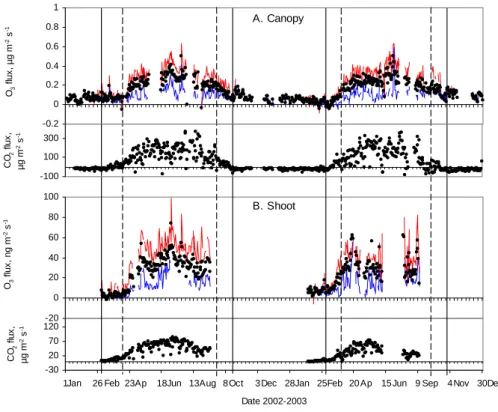
seasonal pattern (Fig. 1). O3 deposition followed the
sea-sonal changes of CO2 exchange (as a proxy of plant
activ-ity): it reached a maximum during summer, low values dur-ing winter and rised and declined in sprdur-ing and autumn. In-spection of the time series suggested that other processes in addition to the plant uptake can control the magnitude and pattern of O3deposition. This fact was more noticeable from
the start of the winter dormancy to the onset of the spring re-covery, seasons when the plant activity is at minimum and is not expected to govern the deposition. When CO2
ex-change reaches a minimum in autumn the deposition actually increases slightly before slowly declining. During winter the deposition is sustained at a level around 20% of the average summer level and rises sharply at the starting of the grow-ing season, similarly as in Keronen et al. (2003). Compar-atively, during summer, the vigorous plant activity seems to dominate O3deposition – likely through stomatal uptake. A
-0.2 0 0.2 0.4 0.6 0.8 1 O 3 fl u x , µ g m -2 s -1
Jan Feb Ap Jun Aug Oct Dec Jan Feb Ap Jun Sep Nov Dec -20 0 20 40 60 80 100 O 3 fl u x , n g m -2 s -1 -30 20 70 120 CO 2 fl u x , µg m -2 s -1 1 26 23 18 13 8 3 28 25 20 15 9 4 30 Date 2002-2003 A. Canopy B. Shoot -100 100 300 CO 2 fl u x , µg m -2 s -1
Fig. 1. Annual patterns of daily O3and CO2fluxes in SMEAR II during 2002-2003 measured at (a) canopy and (b) shoot scale. Positive values denote uptake by the plant. Black dots are values of whole-day averaged fluxes. Lines are day (red) and night (blue) averaged O3 flux.The flux of CO2relates to the intensity of forest activity. Seasons are also marked by the vertical lines (dashed ) the start and end of the thermal growing season, daily mean temperature >5◦C; and (solid): the start and end of thermal winter, daily mean temperature <0◦C.
salient feature is the existence of a remarkably non-constant nocturnal deposition as shown by the night time averaged fluxes in Fig. 1.
Details of the range and daily pattern of the O3deposition
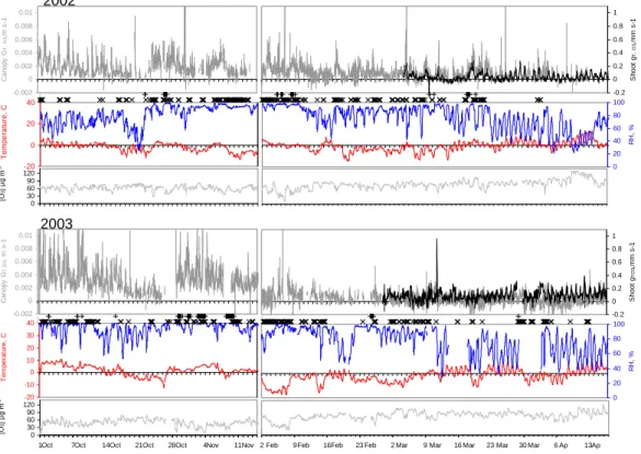
(Figs. 2–3) show a change in behaviour that is mostly ex-plained by the intensity of plant activity and concurrent mois-ture regime. At the transit from autumn to winter and from winter to spring (Fig. 2), the level of deposition remains low and the limits of the growing season are marked by the ap-pearance/disappearance of the daily pattern of O3deposition
(in general, maxima during day and minima during night). Moisture-related higher levels of deposition are seen on both years at the onset of the thermal winter as an increase in the general level of deposition that coincides with precipitation events and/or generally moist conditions. During the winter months deposition is sustained and seems to vary due to a combination of moisture and temperature changes. Temper-ature fluctuates around 0◦C and the move into minus temper-atures coincides with decreases on the deposition level.
Spring is the driest time of the year at this boreal site (cf. Fig. 4). This is reflected in the almost inexistent noctur-nal O3deposition during this season and an average level of
deposition smaller than during winter, a fact that is specially clear during spring 2002 (cf. Fig. 2). Spring 2003 behaves slightly different: O3deposition at the canopy-scale remains
generally low and correspondence with moisture or tempera-ture is less obvious, which suggests the deposition during this period might be related to some other environmental factor. Scrutiny of the complementary measurements showed that the air masses during that period were more polluted (av-erage daily concentration during summer, spring 2002, and spring 2003 were for NOx1, 2–4, and 5–8 ppb, and for SO2
were 0.3, 1, and 2–4 ppb, respectively).
During the growing season, the situation is less ambiguous (Fig. 3): the general level of O3deposition at both scales
cor-responds well with the ambient RH , not with temperature. In general, during drier periods there is a marked diurnal pattern with a daily maximum and nocturnal minimum whereas this cycle is lost during moist conditions. This behaviour is illus-trated during extended warm periods that happened in both summers: during the warm and dry July of 2002 deposition level show a clear daily pattern and a lower maxima com-pared to the warm and moist July of 2003.
3.1.1 Wetness and humidity conditions
The conditions we are referring as moist represent in fact a variety of situations which depend also whether we refer to the ambient air or to the foliage surface. Rainfall wets the foliage surface directly. The droplet detector indicates that
-0.002 0 0.002 0.004 0.006 0.008 0.01 C a n opy G T, O 3 , m s -1 -20 -10 0 10 20 30 40 T e m p er at ur e, C 0 30 60 90 120 [O 3 ] µ g m -3 0 20 40 60 80 100 RH , % -0.2 0 0.2 0.4 0.6 0.8 1 S hoot g TO 3,m m s -1
1Oct Oct Oct Oct Oct Nov Nov Feb Feb Feb Feb Mar Mar Mar Mar Mar Ap Ap7 14 21 28 4 11 2 9 16 23 2 9 16 23 30 6 13
-0.002 0 0.002 0.004 0.006 0.008 0.01 C a n opy G T, O 3 ,m s -1 -20 0 20 40 T e m p erat u re , C -0.2 0 0.2 0.4 0.6 0.8 1 S h oot g T, O 3 ,mm s -1 0 20 40 60 80 100 RH , % 2002 2003 0 30 60 90 120 [O 3 ] µ g m -3
Fig. 2. Time series of O3conductance and environmental factors during autumn and spring 2002–2003. Ozone conductance for the canopy (grey) and shoot (black). In addition of temperature (red) and RH (blue) we also mark the recorded fog episodes (+) and (X) droplet detection, to signal the occurrence of general moist conditions. Ozone ambient concentration is also shown.
-0.002 0.003 0.008 0.013 0.018 C anopy G T.O 3 , m s -1 -0.2 0.3 0.8 1.3 1.8 S h oot g TO 3 , m m s -1 -0.002 0.003 0.008 0.013 0.018 C anopy G T, O 3 , m s -1 -0.2 0.3 0.8 1.3 1.8 S hoot g TO 3, m m s -1 0 10 20 30 40 T e m p e rat ure, C 0 20 40 60 80 100 RH , % 0 10 20 30 40 T e m p er a ture, C 0 20 40 60 80 100 RH , %
18Ap May May June June July July July Aug Aug Sep Sep 2 17 1 16 1 16 31 15 30 14 29
2002 2003 0 30 60 90 120 [O 3 ] µ g m -3 0 30 60 90 120 [O 3 ] µ g m -3
Fig. 3. As in Fig. 2 but during the growing season.
0 20 40 60 80 100 F requenc y % droplets surface w etness 0 20 40 60 80 100 1 2 3 4 5 6 7 8 9 10 11 12 1 2 3 4 5 6 7 8 9 10 11 12 Time, months 2002-2003 F requenc y , % <50 50-70 70-80 80-95 >95
A
B
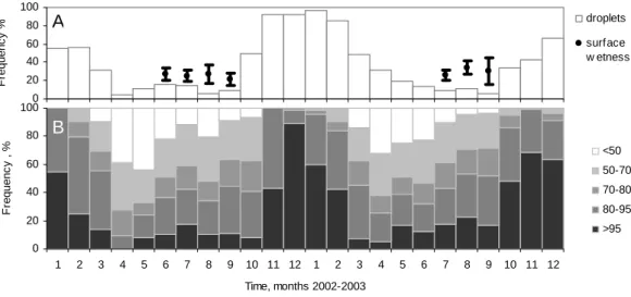
Fig. 4. The frequency occurrence of wetness, moisture and humidity, during 2002–2003. Monthly valuates of (a) Presence of wetness on the
foliage according to SW sensors (average ±SD of all sensors in the canopy) and occurrence of rainfall/snowfall according to droplet detector (note that the “drops” detected during winter should be mostly interpreted as snow cover); (b) Relative duration of different categories of ambient RH . 0 1 2 3 4 5 6 7 0 20 40 60 80 100 RH, % S u rf ac e Wet n e s s S e ns o r s ig nal 0 25 50 75 100 125 150 0 20 40 60 80 100 0.0 0.2 0.4 0.6 0.8 1.0 0 20 40 60 80 100 RH, % S u rf a c e We tnes s S e n s or s ign al A B
Fig. 5. The relation between the surface wetness and the ambient relative humidity. Values are 15-min averages for one sensor (a) inside a
chamber (b) outside the chamber in the canopy. For clarity, the signal has been levelled to 0 at the daily minimum value. Grey points show all data during 7 July–15 October 2002 (in the inset for the canopy). The coloured points highlight few-day time series that typify different situations, all of them in the absence of rain: white-sustained dry weather, black-sustained moist weather with occurrence of fog, red-variable weather with mixed situations. Note the signal inside the chamber remains in the lower range.
during the growing season droplets fall between 5 and 30% of the time. When the rainfall stops, the foliage remains wet for some time, as detected by the SW sensor: the foliage is still wet the following 2 to 12 h. This represents at least 10% more time than the rainfall duration (Fig. 4a). The ambient RH (Fig. 4b) varies with the seasons with April-May be-ing the driest months and November–February bebe-ing almost permanently saturated (on account of the low temperatures rather than high water vapour content in the air). The clear-est trend along the growing season is the gradual decrease of very low RH (<50%) and the rise of the highest (>80%)
towards the fall whereas the occurrence of medium values re-mains similar. The water vapour can condense and form fog or mist when the ambient temperature goes below the mea-sured dew point temperature, which happens few to several days per month. During summer these are mainly radiation fogs and otherwise probably evaporative fogs – we assume no guttation from the foliage. By contact with cold surfaces the same conditions lead to dew formation, collection of wa-ter as visible droplets on surfaces.
The ambient humidity gathers on the foliage surfaces also below saturation point, a fact that is detected by the SW
6 A. All summer 0 0.002 0.004 0.006 0.008 0.01 0.012 0.014 0 6 12 18 C anop y G T, O 3 , m s -1
D. Summer during rain
0 6 12 18 0 0.2 0.4 0.6 0.8 1 1.2 1.4 1.6 1.8 2 S hoot g t,O 3 , mm s -1
C.Summer after rain
0 6 12 18
B. Summer dry days
0 6 12 18
shoot canopy
time of day, hours
midnight rain midday rain
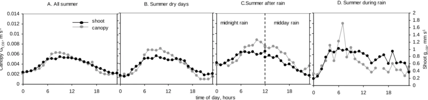
Fig. 6. Diurnal patterns of ozone deposition at canopy and shoot scales under different weather conditions. Hourly values averaged including
2002–2003 thoughtout the periods: (a) mid-April to end of September, and extracted from this period are: (b) 28 dry days, (c) 13 rainfalls ending at midnight ; 10 rainfalls ending at midday, (d) 36 rain events. See the text for explanations. Note the different y-axis range for the different scales, ratio canopy: shoot is 7.
sensor on the foliage enclosed in the gas exchange cham-ber as well as on foliage outside the chamcham-bers (Fig. 5). Ac-cording to the SW response to the ambient RH , there is a moisturising effect at RH >70%, that is – with exception of April–May – at least half of the time (cf. Fig. 4b).
3.2 The effect of rain fall
Rainfall wets the foliage but it does not reach the shoot enclosed in the chamber. We make use of this difference to see how rainfall and raindrops on the foliage affect O3
deposition, since any specific effect should be apparent in the canopy but not in the chamber. In general, the mea-sured O3 deposition on the canopy and on the shoot
pre-sented similar daily patterns with the obvious magnitude dif-ference between scales. The averaged summer values at both scales related to each other approximately in a linear fash-ion (Fig. 6a); similarly during dry summer days (Fig. 6b), although the canopy cycle presents comparatively more am-plitude.
During rainfalls the daily cycle was clearly disrupted in the chamber shoot deposition, which seemed to be generally enhanced compared to the canopy (Fig. 6d). This would sug-gest that while the rain falls the canopy deposition is inhib-ited. Once the rain stopped the drops remained in the foliage during the following hours and the affection to O3deposition
seemed to depend on the timing of the rainfall end. For clar-ity, we chose two groups of rain events: rainfalls that finished either around noon or around midnight, and considered the immediate 12 h after. During the afternoon, O3 deposition
towards the wet canopy was enhanced whereas the cham-ber shoot deposition was not, the implication being that rain drops enhanced O3deposition. After a midnight rain, both
canopy and chamber shoot deposition were higher than their averages, so since the shoot deposition was also enhanced we can not conclude the deposition enhancement would be due to the drops.
To fully interpret these observations, however, it is not enough to consider the presence or absence of rain drops on the foliage. There is one condition, RH , that varies with the timing of rain and explains the rise in the shoot O3
deposi-tion inside the chamber despite the absence of drops. Canopy can be wet in the afternoon when the ambient RH remains low; but RH remains close to 100% when a canopy is wet through the night and early morning or while it is actually raining whatever the time of the day. High RH does occur also inside the chamber and increases the sink strength of O3
deposition after a nighttime rainfall.
3.3 Stomatal uptake and non-stomatal sink
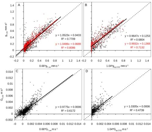
During conditions when surface moisture is supposedly at minimum – what we have termed dry conditions – we found a good agreement between the estimations of stomatal uptake and the measured deposition (Fig. 7). In all cases, the slopes of the linear regression were close to 1. At both scales, the measured total conductance (gT ,O3, GT ,O3)was only slightly
better explained (larger r2) by the estimation of stomatal conductance through the water vapour conductance (gsto,wv,
Gsto,wv)than from the conductance obtained with the
photo-synthesis model (gsto,CO2, Gsto,CO2).
For the canopy scale, an underestimation of GT ,O3 from
the canopy integrated photosynthesis model was expected because Gsto,CO2only described the contribution of the pine
foliage. This was actually the case when all the conditions were considered (data not shown), but it does not come ob-vious in the analysis of data during only dry condition
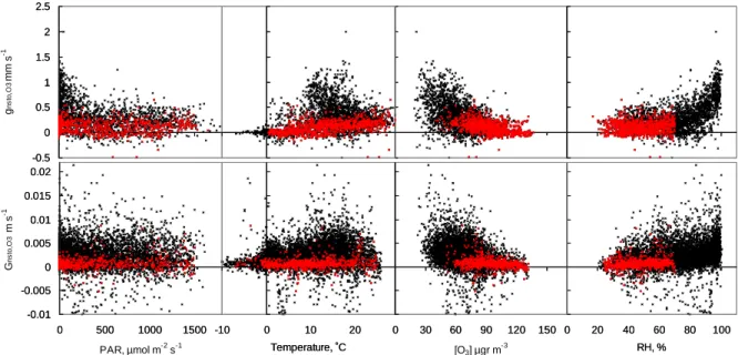
Under the whole range of ambient conditions, we found disagreement between the values of the estimated and mea-sured ozone conductances. According to Eqs. (3) and (4), this difference represents the non-stomatal sink, gnonsto,O3 or Gnonsto,O3.
The relationship of these differences with the environmen-tal variables is shown in Fig. 8. When all data is considered, the bigger differences take place at low irradiance, low ozone
Fig 7 y = 1.0523x + 0.0433 R2 = 0.7709 y = 1.0486x + 0.0688 R2 = 0.8086 -0.2 0 0.2 0.4 0.6 0.8 1 1.2 1.4 -0.2 0 0.2 0.4 0.6 0.8 1 1.2 1.4 0.66*gT ,wv mm s-1 gT,O 3 mm s -1 y = 0.9932x + 0.1368 R2 = 0.7132 y = 0.9647x + 0.1253 R2 = 0.6804 -0.2 0 0.2 0.4 0.6 0.8 1 1.2 1.4 1.04*gop,CO2 mm s-1 A B y = 1.0305x + 0.0006 R2 = 0.4739 -0 0 0.002 0.004 0.006 0.008 0.01 0.012 0.014 1.04*Gop,CO2 m s-1 y = 0.9775x + 0.0006 R2 = 0.6172 -0.002 0 0.002 0.004 0.006 0.008 0.01 0.012 0.014 -0 0 0.002 0.004 0.006 0.008 0.01 0.012 0.014 0.66*GT ,wv m s-1 GT, O 3 m s -1 C D
Fig. 7. Regression between measured and calculated ozone conductance from the estimation of water vapour (a, c) and CO2conductance (b,
d) during dry conditions. (a–b): shoot values hourly averaged, for April–September 2002 and 2003. Colours denote different shoots. (c–d):
half hourly canopy values for 2002–2003. Diagonal is the 1:1 line.
Table 1. Magnitude of stomatal and non-stomatal conductances.
Non-stomatal conductance was estimated according to Eq 3 and 4 using the stomatal conductance estimated from the photosynthesis conductance model. Average values from April to September; the different rows in the shoot data correspond to different shoots. Val-ues of the standard deviation are of the same magnitude than the averages, omitted for clarity.
Average conductance % of gnonsto,O3
mm s−1 from total
dry moist dry moist dry moist
gsto,O3 gnonsto,O3 Shoot 2002 0.08 0.15 0.08 0.21 50 58 0.18 0.36 0.11 0.36 38 50 0.18 0.37 0.12 0.33 40 47 2003 0.20 0.30 0.08 0.30 29 50 0.16 0.21 0.11 0.22 41 51
Gsto,O3 Gnonsto,O3 % of Gnonsto,O3
from total
Canopy 2002 0.9 1.73 0.65 2.44 42 59
2003 0.89 1.49 0.29 2.75 25 65
concentration, and high ambient relative humidity; three cir-cumstances that coincide in time. However, we find these bigger values at the mid-range of the recorded temperature.
The patterns at the canopy scale are more diffuse but are consistent with the trends showed by the shoot-scale data. For comparison, Fig. 8 also shows the smaller set of data representing drier conditions that was depicted in Fig. 7. In this case, there is a general lack of pattern except the shoot data would imply a correlation with temperature.
Table 1 summarises the magnitude of the estimated O3
conductances considering the stomatal and non-stomatal components under dry and moist conditions. On average, at the shoot scale both components have similar magnitudes. During moist conditions they are both larger than during drier conditions, by a factor of 1.4 for gsto,O3 and 2 for gnonsto,O3.
The contribution of the non-stomatal component is around 50% under moist conditions for all shoots, and slightly lower and more variable under dry conditions. The averages in Ta-ble 1 shows variation between shoots and years; most no-tably the shoots measured during 2003 seem to have weaker non-stomatal sink in dry conditions than in the previous year. Reasons can be found in the younger age of the foliage (one-year old in 2003 and two-year old in 2002) and in the fewer dates available for the average (the standard deviation is larger in 2003). Interestingly, the canopy scale also dis-plays a weaker non-stomatal sink in dry conditions during 2003. Otherwise, the non-stomatal contribution to the total canopy sink is 60% (dry) or larger (moist).
-0.01 -0.005 0 0.005 0.01 0.015 0.02 0 500 1000 1500 G ns to, O 3 m s -1 -0.01 -0.005 0 0.005 0.01 0.015 0.02 0 500 1000 1500 PAR, µmol m-2 s-1 -10 0 10 20 Temperature, ˚C -10 0 10 20 Temperature, ˚C 0 20 40 60 80 100 RH, % 0 20 40 60 80 100 RH, % -0.5 0 0.5 1 1.5 2 2.5 g ns to, O 3 mm s -1 -0.5 0 0.5 1 1.5 2 2.5 0 30 60 90 120 150 0 30 60 90 120 150 [O3] µgr m-3
Fig. 8. Regression of the non-stomatal O3sink against the range of various environmental factors. Non-stomatal conductance according to Eqs. (3) and (4) using the stomatal conductance estimated from the photosynthesis conductance model (the shapes are similar in case of estimation from water vapour flux). Data March–September 2002 from one shoot (hourly averages) and the canopy (half-hourly averages). Black: all data, Red: data during dry conditions as in Fig. 7.
3.4 Non-stomatal shoot deposition relation with ambient RH and temperature: a role for surface moisture
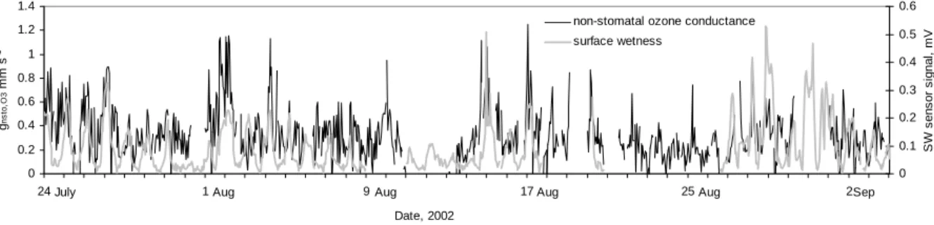
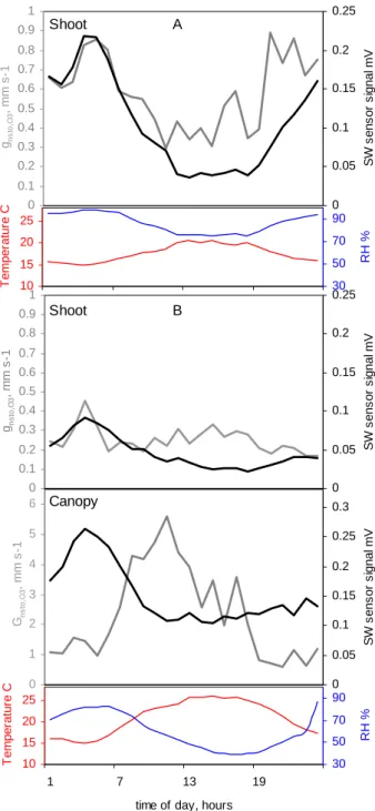
Whether the apparent relation of non-stomatal ozone deposi-tion with ambient RH relates to changes at the surface of the foliage we have checked with simultaneous measurements of surface moisture and gas exchange on the same shoot inside the gas exchange chamber. We found similitude in the two temporal patterns (Fig. 9), but it was also clear that the de-gree of accordance was not consistent between days. Day by day linear regression yielded stronger and weaker agree-ments (0.1<r<0.8) and almost one order of magnitude range in the slope, although the correlation was indeed predomi-nantly positive. A similitude in temporal patterns also ap-peared in the averaged daily development (Fig. 10). There was a coincidence between the highest peak of RH , the SW signal and the difference between predicted and measured ozone deposition The rise on ozone conductance happened on average a couple of hours earlier than the rise of stom-atal conductance and it coincided with the rise in surface wetness. During days with higher RH we found coincident morning and evening maxima in the surface wetness and the non-stomatal ozone deposition. During drier days the coin-cident maximum appeared only in the morning but was also evident in the canopy scale deposition.
It is conceivable that aqueous films gather at the surface of the needle and modulate the surface sink. This sink would then follow a pattern that reflects the film formation and the ozone decomposition mediated by it. The flux generated by such sink can be expressed:
Flux=ϕ · 8 (5)
where ϕ refers to the relative amount of water on the surface and φ relates to the chemical rate of ozone decomposition.
The behaviour of the surface moisture on the foliage as detected by the SW sensor (Fig. 5) can be considered the expression of the adsorption of vapour on the surface, and would suggest a process of the type described by BET ad-sorption isotherms (Adamson, 1960). We calculated ϕ as the relative coverage predicted from the BET isotherm (D1) and found indeed that the calculated ϕ and the measured SW agree with correlation coefficients r>0.8 most of the days. The value of ϕ was 1 at 70%RH , 2 at 85%RH , and raised sharply over 5 towards 100%RH .
The relation to the estimated non-stomatal ozone sink gnonsto,O3 (m s
−1)would be:
gnonsto,O3 =ϕ · V
Aκ (6)
where V , and A as in Eq. (1), κ is the rate constant of the chemical reaction that results in the O3removal,
decomposi-tion or scavenging, and it has units s−1as a chemical reaction of order 1. From Eq. (6) we extracted the value of κ, which is not enhanced by the ambient RH and displays the temper-ature relation typical of a chemical reaction rate (Fig. 11).
4 Discussion
4.1 Observation of ozone deposition and moisture effects In studies attempting to analyze the complex interactions be-tween ecological and physical factors, continuous long-term
0 0.2 0.4 0.6 0.8 1 1.2 1.4 24 1 9 17 25 2 Date, 2002 gns to ,O 3 mm s -1 0 0.1 0.2 0.3 0.4 0.5 0.6 S W s e ns o r s ign al , m V
non-stomatal ozone conductance surface wetness
July Aug Aug Aug Aug Sep
Fig. 9. Times series of hourly averages from chamber measurements on one shoot. Comparison between the calculated non-stomatal ozone
conductance (black) and the surface wetness signal (grey) for two different types of weather conditions, wetter (a) and drier (b). Canopy data is only shown for the drier case.
recordings in the field are irreplaceable in order to gather in-formation under the various environmental situations in the frequency and intensity they happen in nature. The simulta-neous measurement of many factors and phenomena allows the observation of correlations in the behaviour of their re-spective time series. We have therefore been able to relate the episodes of ozone deposition enhancement with the pre-vailing moisture regime at the site from the observation of the recorded time series. High time resolution was also an advantage to analyse episodic situations such as rainfalls as the capture of these somewhat more random occasions was maximised.
There are micrometeorological field studies that examined the non-stomatal ozone deposition to vegetation but did not consider or detect the effect of surface moisture. These stud-ies do not contradict the possibility of moisture enhancement rather they just did not focus on examining it. Whether the effect of the moisture was reported or not might have de-pended on whether the measurements included or not periods of high RH and whether the subsequent analysis allowed its discrimination The correlation with radiation and tempera-ture reported in Fowler et al. (2001) was based on day-time dry-conditions data, and Goldstein et al. (2004) used day-time means in their suggestion that non-stomatal ozone de-position was controlled by temperature through terpene oxi-dation. The highest ambient RH during any certain day hap-pens during night and at sunrise. Since a high time resolution in the data is needed in order to capture this, the use of av-eraged data probably obscures the effect. Such could have been also the case in Mikkelsen et al. (2004) where the sea-sonally grouped 5-year averages of nocturnal ozone deposi-tion is found to relate linearly with temperature. Chemical quenching was also considered important by Mikkelsen et al. (2000) on account of a simultaneous increase in terpene emission and ozone deposition, although the data also shows a many-fold enhancement of deposition during a low emis-sion cloudy day. The higher values measured after sunrise they relate to BVOCs (biogenic volatile organic compound) but they could as well be related to the higher RH at sunrise.
In accordance with our results, the majority of studies that have directly investigated the effect of wetness on O3
deposi-tion found actually an enhancement effect (see Introducdeposi-tion and Massman 2004). There are some reports of inhibition, which mainly refer to total canopy parameters including di-urnal data. For example, Grantz et al. (1997) reported re-duced O3canopy flux and Vdupon dewfall on a cotton field
but argued that it was mainly due, not to a reduction of the non-stomatal sink, but to a reduction of the stomatal uptake due to droplets blocking the stomatal pores. Such effect be-comes apparent from measurements of canopies formed by amphistomatous-leaf species (stomata on both sides of the leaf) such as cotton. The same would apply to maize (We-sely et al., 1978; Leuning et al., 1979), wheat (Hicks, 1987) and poplar (Fuentes et al., 1994).
Zhang et al. (2002) present a recent effort in the study of the non-stomatal conductance to O3 flux. They concluded
that not only dew and rain but also high ambient RH in-creased the O3 deposition to the canopy. The correlations
presented in their study, e.g. RH vs. canopy resistance, are weak (r<0.5) but nonetheless their suggestion regarding the modulation of the non stomatal conductance by RH seems to be valid, according to our own results. Their parame-terized nightime canopy O3deposition for mixed forests is
within the range of our observed values i.e. an average of around 0.001 m s−1for dry canopies and 0.003 m s−1for wet canopies. A thorough analysis of O3deposition for a conifer
forest is presented in Carrara 1998 and Lamaud et al., 2002. They did not measure the surface wetness directly but instead applied a data selection based on the ambient RH consider-ing foliage was dry at less than 70% and dew-wet at more than 95% RH . They reported that the non-stomatal O3
de-position on a dry canopy is negligible but that there is a clear enhancement on dew-wet foliage, and concluded the effect was stronger than the stomata uptake and independent of the dynamical turbulence.
The relevance of the moisture to the O3deposition at any
certain location depends of course on the particular envi-ronment under consideration. In dry and arid regions the
0 1 2 3 4 5 6 Gns to ,O 3 , m m s -1 0 0.05 0.1 0.15 0.2 0.25 0.3 S W s ens or s ignal m V 0 0.1 0.2 0.3 0.4 0.5 0.6 0.7 0.8 0.9 1 gns to ,O 3 , m m s -1 0 0.05 0.1 0.15 0.2 0.25 S W s ens or s ignal mV 10 15 20 25 1 7 13 19
time of day, hours
T e m per at ur e C 30 50 70 90 RH % 10 15 20 25 T e mper atur e C 30 50 70 90 RH % A B 0 0.1 0.2 0.3 0.4 0.5 0.6 0.7 0.8 0.9 1 gns to ,O 3 , m m s -1 0 0.05 0.1 0.15 0.2 0.25 S W s ens or s ignal m V Shoot Shoot Canopy
Fig 10
Fig. 10. Daily patterns of gnonsto,O3, surface wetness, RH and temperature. (a) moist conditions , 20–26 July 2002 and (b)) dry conditions, 12–18 July 2002. Data correspond to one of the shoots and the attached surface wetness sensor.
non-stomatal sink represents a significant proportion of the O3 deposition, e.g. as recorded at Mediterranean locations
(Cieslik, 2004). High air humidity regimes are rarer and sur-face moisture potentially less relevant, thus this sink is not likely related to surface wetness and would be instead modu-lated by different factors. Moisture enhancement would also not be expected to happen in freezing conditions and there-fore it does not explain the substantial deposition of O3
dur-10 -0.01 0 0.01 0.02 0.03 0.04 0.05 0.06 0.07 0.08 -10 0 10 20 30 Temperature C k s -1
Fig. 11. Relation between temperature and the estimated chemical
destruction rate according to Eqs. (5)–(6) as a 1st-order reaction rate.
ing winter at our site (Figs. 1–2, Keronen et al., 2003).Winter deposition implies a certain amount of removal might happen by contact to the frozen surfaces. At least the snow pack is believed to be an efficient sink for O3(Albert et al., 2002).
4.2 Approaches to ozone deposition parameterization Early parameterisations are based on tabulated values to be applied to different conditions. The detailed parameterisa-tion of Wesely (1989) took into account the characteristics of different gases according to their reactivity and solubil-ity and incorporated the effects of dew and rain. Zhang et al. (2002) proposed a parameterisation for the non-stomatal sink of ozone that introduced a moisture enhancement as determined by ambient relative humidity, canopy leaf area index and friction velocity, although without being explicit about the mechanistic details. The recent multilayer bio-chemical deposition by Wu et al. (2003) incorporates the thickness of the water film on the leaf and its pH to describe the O3conductance to a wet leaf; this study is thus more
de-scriptive although is based on empirical equations.
The lack of understanding on the mechanism driving O3
deposition to the wet foliage hinders its quantification and leads to its parameterization as constant values (Ganzeveld and Lelieveld, 2004). It seems that the amalgam of con-tradicting results and multiple apparent influences have ren-dered the parameterisation of the non-stomatal ozone sink elusive. This is particularly so for regional-scale models comprising many different vegetation types. For exam-ple the newest EMEP methodology applies a humidity fac-tor derived from Klemm et al. (2002) that is applied to a soluble gas such as SO2 but not to O3. An evaluation
of this model against long-term micrometeorological data from a spruce forest and moorland showed a large unex-plained variation in the surface conductance during the pe-riod when non-stomatal deposition dominates and suggested that these discrepancies might well be related to surface
ness (Tuovinen et al., 2004). Our results indicate that mois-ture significantly modulates the non-stomatal sink, suggest-ing that model results could indeed be improved by incorpo-rating this effect in the parameterisation of non-stomatal sur-face conductance, particularly in the regions that frequently experience high moisture regimes.
4.3 Analysis of the ozone deposition
The present approach to partition the O3canopy deposition
is similar to other studies. The surrogation approach is com-mon to most studies, i.e. scaling from the flux of another gas, typically water vapour. At the canopy scale, extracting the non-stomatal deposition via the three resistance analogue is an extended practice (e.g. Fowler et al., 2001; Gerosa et al., 2004; Lamaud et al., 2002). Some studies have used a multilayered or more sophisticated canopy model (e.g., Amthor et al., 1994; Kurpius and Goldstein, 2003; Zeller and Nikolov, 2000) but essentially followed the surrogation principle. Some authors have limited the analyses of the non-stomatal deposition to nocturnal measurements of total O3
fluxes (e.g. Mikkelsen et al., 2004). Whatever the case, the surface resistance is obtained as a residual, i.e., as the differ-ence between the measured total deposition and the aerody-namic and viscous resistances (cf. A.1) and such value accu-mulates unaccounted errors and is affected by the parameter-isation of the atmospheric resistance Ra, and particularly Rb
(Tuovinen et al., 1998).
Our treatment of the canopy scale O3fluxes does not
per-mit a complete partition of the canopy O3sinks, particularly
the role of the understory is poorly defined. Nonetheless, the results show the pine foliage uptake represents only a fraction of the total deposition. Based on the percentages on Table 1, a rough estimation of the contribution of the undestory sink would be around 12% in 2002 and 20% in 2002. Lamaud et al. (2002) found even larger proportion of the ozone deposi-tion to happen in the understory.
4.3.1 Canopy versus shoot
Previous analysis at the shoot scale (Altimir et al., 2004) showed the potential role of RH as a modulator of non-stomatal ozone sink and the present work shows the same phenomenon is observed at the canopy scale. We then used the shoot scale measurements to further analyse the possible mechanisms of the apparent RH enhancement. We observe the ozone fluxes at canopy and shoot scale with no attempt to scaling between them. Nonetheless, a direct comparison of the values tells the difference is around one order of mag-nitude and the ratio canopy:shoot is 7 (e.g. Fig. 6), a value that approaches the average LAI of the site. Also, it does seem that O3deposition measured at both scales is affected
similarly by the prevailing conditions although in principle a single shoot and a whole canopy represent aggregates that include different components.
4.3.2 Stomatal versus non-stomatal
The principal purpose in the wording of stomatal and non-stomatal is to reflect the partitioning of the ozone flux be-tween the portion that passes through the stomatal pore (stomatal) and that which does not (non-stomatal). This divi-sion is implicitly connected with the interest to know whether the ultimate sites of O3removal are in the mesophyll
(stom-atal) or in some other place (non-stom(stom-atal). However, the stomatal and non-stomatal fractions of deposition are not totally independent. Methodologically, since temperature, light, and VPD or RH affect both components it becomes in practice difficult to separate the effects on the basis of correlation, a difficulty already commented by Mikkelsen et al. (2004). Phenomenologically, the interrelations of all the components at the leaf-air interface are tight and e.g. the evaporation of surface water vapour and the emission of BVOC affect the so-called non-stomatal deposition and can be themselves dependent of the stomatal conductance.
In the methodology we have used, the estimated values of non-stomatal deposition are, numerically speaking, evi-dently dependent on the estimation of the stomatal compo-nent, which is approached via the behaviour of water vapour or CO2. Strictly speaking though, the estimated conductance
is likely to be a composite conductance and not a direct proxy of the stomatal aperture. In the case of the estimation of water vapour conductance from the measurements of water vapour exchange the cuticular evapotranspiration is actually included. The relation between the amount of surface mois-ture and the evaporation from the cuticular surface is obvi-ous. The relation can be tightened further with the possibility that the transpired water vapour contributes to the gathering of surface moisture detected by the SW sensors (Burkhardt et al., 1999). The better agreement in Fig. 7 between O3
and water vapour conductance could be due to the readily inclusion of the surface moisture and/or cuticular transpira-tion in gwv. If the difference between stomatal and cuticular
transpiration and surface wetness evaporation becomes un-clear, so does the discrimination between stomatal and non stomatal O3sinks based on estimations of water vapour
con-ductance. The lower the VPD or the higher the ambient RH the more difficult the distinction becomes. In case of extremely low VPD, also the estimation via photosynthesis-conductance models fails because the assumption of optimal-ity does not necessarily hold due to low evaporative demand, together with the relative inaccuracy in determining VPD. It has been argued that since mesic environments and low VPD conditions favour larger stomatal apertures the cumulative amount of O3deposition at such sites- e.g. temperate and
bo-real zones- would be larger than e.g. at Mediterranean zones (Grulke et al., 2003; Pannek and Goldstein, 2001). However, a destruction of O3at the outer surfaces of foliage promoted
by surface moisture would also increase in moist conditions and prevent a certain portion of the uptake thereby reducing the O3dose into the plant.
4.3.3 Water films on the foliage surface
The SW sensor response to RH recorded in this field study is comparable to the field and laboratory measurements on Norway spruce and Scots pine (Burkhardt and Eiden, 1994). This works showed the hydrophobic nature of the waxes that cover the foliage does not necessarily preclude the formation of water clusters or films. The sorption of water vapour can be prompted by the hygroscopic properties of the salts that are present on the foliage surface or more likely, there is a mixture of salts as well as any certain salt in a mixture of states. Other compounds likely to be on the surface such as oxidized organic compounds could further enhance the ef-fect (Demou et al., 2003). In addition, the foliage surface is structurally intricate and permits that even hydrophobic films could take up water since corrugation on the surfaces enhances water uptake on hydrophobic surfaces (Rudich et al., 2000; Sumner et al., 2004). We have interpreted the SW-RH relationship as water vapour adsorption on the foliage surface and have represented it according to a BET adsorp-tion isotherm. The case is clearly not a homogeneous mul-tilayered adsorption but one where adsorption is facilitated by deliquescence and capillary condensation (Eiden et al., 1994). The value of ϕ, as well as the SW signal, is related to the thickness of the water film although not strictly related to the number of water molecules stacked up in the film.
Existing estimations of the thickness of water films on fo-liage report a wide range of values. Van Hove and Adema (1996) determined the thickness of the apparent water layer on leaves to be between 10–100 µm corresponding to low-high humidity conditions, based on the calculation of NH3
adsorption and chamber measurements on bean and poplar (van Hove et al., 1989). According to Burkhardt and Ei-den (1994), water films are in the order of 1–50 nm during day, based on their estimation of particle load on spruce fo-liage and the absorbed water mass by particles. A similar approach was used on a model of NH3exchange by Flechard
et al. (1999), who considered the amount of liquid water held on the surface of a moorland canopy varied between 100 nm to 1 mm. They also monitored leaf wetness with SW sensors and saw transient rise in the sensor signal as leaves started to dry that were not reflected in the estimated amount of leaf surface water. They considered that the increase in concen-tration of ions upon evaporation increased the solution con-ductivity and produced the signal rise. We did not detect such phenomena on our SW canopy measurements, a fact that could be partially due to the different particle load between the two sites. Sites differences in SW retention appeared in the measurements of Klemm et al. (2002), as grasslands gathered and retained surface moisture longer than forests. The variability was not discussed in terms of species but at-tributed to different exposure to high RH due to orographic regime and to different pollution load on the foliage surfaces. There are many possible contributors to the build up of surface films on the foliage and this rather complicates the
survey of the compounds actually involved in film forma-tion and hinders possible simulaforma-tion. Addiforma-tionally, knowl-edge about the detailed spectra of compounds involved might be necessary also to understand how surface moisture modu-lates the ozone deposition, since the chemical composition of the film is likely relevant to O3 scavenging reactions.
For example, the chemistry of the solution formed on wet maple leaves is more reactive to O3than the one formed on
poplar leaves (Fuentes et al., 1994). Also different mecha-nisms of O3decomposition are expected to happen in acidic
or alkaline solutions (Sehersdted et al., 1991), a fact appar-ent in the material-specific behaviour reported in GrØntoft et al. (2004).
The values of a supposed chemical reaction reported in Fig. 11, in the order of 10−2s−1, are large compared with published values of first order chemical removal. Bulk chemical O3removal from material studies reports rates in
the range of 10−5 (GrØntoft et al., 2002). Sehersdted et al. (1991) reports reaction rates in the range of 10−4s−1 (at 30◦C) for decomposition of O3 in acidic aqueous
solu-tions and Hsu et al. (2002) offers k=3.77×10⁸e(−7025/T ) min−1 (2.4 10−4s−1at 20◦C). First order rate constant for
O3 removal averaged 8.8 10−3s−1 – thus a slightly larger
value – for a solution with a variety of hydrophobic organic acids (Westerhoff et al., 1999). Unimolecular decomposi-tion reacdecomposi-tions are also expressed as a second-order rate phe-nomena; in such case κ from Eq. (6) would range around 10−14cm3molecules−1s−1. This is also larger value than the reported rates of gas O3 thermal decomposition which
are in the range of 10−26cm3molecules−1s−1(e.g., Benson et al., 1957; Heimerl and Coffe, 1979). This comparison with available rates of O3decomposition suggest that such
reac-tion alone can not account for the level of chemical scaveng-ing presumed from the values in Fig. 11.
4.4 Other possible mechanisms
In this study, the portion of ozone deposition that the cal-culated stomatal uptake can not account for is related to the ambient RH , possibly via the ozone reaction with the liq-uid films on the foliage surface. There are other elements and possible mechanisms of ozone scavenging that deserve further scrutiny.
4.4.1 Nocturnal uptake
Many conclusions on the non-stomatal sinks have been drawn from nigthtime data based on the assumption that the stomatal conductance was negligible and therefore all noc-turnal deposition was non-stomatal. Such assumption is also important in our study because although we analyse both di-urnal and noctdi-urnal data, the effect of RH is more promi-nent at night. During night time, stomatal uptake of O3 in
C3 plants is often assumed to be zero, negligible or small on account of the lack of light resulting in the closure of