HAL Id: insu-02397197
https://hal-insu.archives-ouvertes.fr/insu-02397197
Submitted on 16 Dec 2020HAL is a multi-disciplinary open access archive for the deposit and dissemination of sci-entific research documents, whether they are pub-lished or not. The documents may come from teaching and research institutions in France or
L’archive ouverte pluridisciplinaire HAL, est destinée au dépôt et à la diffusion de documents scientifiques de niveau recherche, publiés ou non, émanant des établissements d’enseignement et de recherche français ou étrangers, des laboratoires
Two-dimensional model for the martian exosphere:
Applications to hydrogen and deuterium Lyman α
observations
D. Bhattacharyya, Jean-Yves Chaufray, M. Mayyasi, J.T. Clarke, S. Stone,
R.V. Yelle, W. Pryor, Jean-Loup Bertaux, Justin Deighan, S.K. Jain, et al.
To cite this version:
D. Bhattacharyya, Jean-Yves Chaufray, M. Mayyasi, J.T. Clarke, S. Stone, et al.. Two-dimensional model for the martian exosphere: Applications to hydrogen and deuterium Lyman α observations. Icarus, Elsevier, 2020, 339 (15 March), pp.art. 113573. �10.1016/j.icarus.2019.113573�. �insu-02397197�
Two-Dimensional Model for the Martian Exosphere: Applications to
1
Hydrogen and Deuterium Lyman α Observations
2 3
D. Bhattacharyya1, J. Y. Chaufray2, M. Mayyasi1, J. T. Clarke1, S. Stone3, R. V. Yelle3, W.
4
Pryor4, J. L Bertaux2, J. Deighan5, S. K. Jain5, and N. M. Schneider5
5 6
1. Center for Space Physics, Boston University, 725 Commonwealth Avenue, Boston MA
7
02215, USA
8
2. LATMOS/CNRS, 78280 Guyancourt, France
9
3. Lunar and Planetary Laboratory, University of Arizona, 1629 E University Blvd., Tucson
10
AZ 80092, USA
11
4. Science Division, Central Arizona College, Coolidge, AZ 85128, USA
12
5. Laboratory of Atmospheric and Space Physics, Boulder, CO 80303, USA
13 14 15 16 17 To be submitted to Icarus 18 19 20 43 Pages 21 1 Table 22 7 Figures 23 24 25 26 27 28 29 30
Proposed running title: 2-D radiative transfer model for Mars
31 32
Corresponding author address:
33
Dolon Bhattacharyya 34
Center for Space Physics 35 Boston University 36 725 Commonwealth Avenue 37 Boston MA 02215, USA 38 e-mail: [email protected] 39 40 41 42 43 44 45 46 47 48 49 50 51 52 53 54 55 56 57 58 59 60 61
Abstract
62
The analysis of Lyman α observations in the exosphere of Mars has become limited by the 63
assumption of spherical symmetry in the modeling process, as the models are being used to analyze 64
increasingly detailed measurements. In order to overcome this limitation, a two-dimensional 65
density model is presented, which better emulates the density distribution of deuterium and 66
hydrogen atoms in the exosphere of Mars. A two-dimensional radiative transfer model developed 67
in order to simulate multiple scattering of solar Lyman α photons by an asymmetric, non-68
isothermal hydrogen exosphere, is also presented here. The models incorporate changes in density 69
and temperature structure of the martian atmosphere with radial distance and solar zenith angle. 70
The 2-D models were applied to the MAVEN-IUVS echelle observations of deuterium and 71
hydrogen Lyman α as well as HST Lyman α observations of hydrogen at Mars. The asymmetric 72
2-D model provided better fits to the data and smaller thermal escape rates in comparison to the 73
symmetric 1-D model for the exosphere of Mars. However, intensity differences between both 74
models became small above ~2.5 martian radii indicating that the exosphere of Mars approaches 75
spherical symmetry at higher altitudes, in agreement with earlier studies. In addition, a new cross 76
calibration of the absolute sensitivities of two instruments on the Hubble Space Telescope and the 77
MAVEN-IUVS echelle mode is presented based on near-simultaneous observations of the 78
geocorona and Mars. 79 80 81 82 83 84 85 86 87 88 89 90 91
Keywords: Mars; Atmosphere; Ultraviolet observations; Radiative transfer
1. Introduction
93
Resonantly scattered solar Lyman α photons by martian exospheric hydrogen have been studied 94
for decades before the transition into 21st century [Barth et al., 1969, 1971; Anderson and Hord,
95
1971, 1972; Babichenko et al., 1976; Dostovalov and Chuvakhin, 1973]. This Lyman α emission 96
at 1215.67 Å was observed to extend to very high altitudes, beyond 30,000 km (~ 8.8 RMars) [Barth
97
et al., 1969]. Photochemical modeling indicated that most of the exospheric H atoms originated 98
from the photo-dissociation of water vapor by ultraviolet sunlight close to the planet’s surface 99
[Hunten and McElroy, 1970; McElroy and Donahue, 1972; Parkinson and Hunten, 1972]. This 100
realization piqued an interest towards understanding the properties of martian exospheric hydrogen 101
as it could provide an insight into the disappearance of Mars’ water. Since the majority of H atoms 102
at Mars were theorized to be escaping by the thermal mechanism of Jeans escape [Hunten, 1973, 103
1982], knowledge about the density distribution and the temperature of the H atoms was deemed 104
necessary to constrain the present-day escape rate of H/H2O from Mars.
105
Observations of the martian Lyman α emission conducted in the past decade revealed 106
significant seasonal changes in H escape rate, with the peak escape occurring close to Mars’ 107
southern summer solstice (Ls = 270˚) [Clarke et al., 2014; 2017; Chaffin et al., 2014; Bhattacharyya
108
et al., 2015; 2017b; Romanelli et al., 2016; Halekas et al., 2017; Rahmati et al., 2017; 2018]. These 109
large seasonal changes were not expected from earlier photochemical modeling of the martian 110
atmosphere [Hunten 1973; Krasnopolsky 2002], and are believed to be a result of a combination 111
of atmospheric upwelling and dust storm activity lifting water vapor to higher altitudes around 112
Mars’ perihelion [Chaffin et al., 2017; Fedorova et al., 2017; Heavens et al., 2018; Clarke, 2018]. 113
This discovery has implications for understanding the water escape history of Mars. Analysis of 114
the observations also revealed the possibility of the presence of an energetic population of 115
hydrogen along with thermal H in the martian exosphere, which could increase (~factor of 2) the 116
present-day escape rate of hydrogen from Mars [Chaufray et al., 2008; Bhattacharyya et al., 117
2017a]. More recently, an enhancement in martian hydrogen escape was also detected by the 118
Imaging Ultraviolet Instrument (IUVS) [McClintock et al., 2015] onboard the Mars Atmosphere 119
Volatile EvolutioN (MAVEN) spacecraft during a series of strong solar flare events and a coronal 120
mass ejection that swept past Mars [Mayyasi et al., 2018]. These findings about the martian 121
exosphere in the past decade indicate that the water escape scenario at Mars is complicated, and 122
all the significant factors that influence hydrogen escape at Mars have to be modeled, analyzed 123
and studied in detail before an accurate estimate of the timeline of Mars’s water loss is made. 124
Lyman α emission from deuterium at 1215.33 Å, the heavier isotope of hydrogen, on the 125
other hand, has only recently been studied in detail to determine the D/H ratio at Mars [Clarke et 126
al., 2017; Mayyasi et al., 2017b; 2019]. The deuterium to hydrogen ratio is a good indicator of a 127
planet’s water loss in the past through atmospheric escape. The lightest gases from every terrestrial 128
planet in our solar system are slowly evaporating into space. In the case of hydrogen and its heavier 129
isotope deuterium, hydrogen is escaping much faster than deuterium due to the difference in their 130
masses. Such an escape imbalance over long periods of time would enhance the D/H ratio in a 131
planet’s atmosphere, thereby providing an estimate of the amount of atmosphere that has escaped 132
the planet [Bertaux et al., 1993; Krasnopolsky et al., 1998]. 133
Global measurements of D/H ratio through observations of HDO and H2O in the martian
134
atmosphere revealed it to be 6 ± 3 times higher than the standard mean ocean water (SMOW) value 135
(1.5576 × 10⁻⁴) [Owen et al., 1988] indicating an extended history of atmospheric escape from
136
Mars. A more recent measurement of the martian D/H ratio by the Mars Science Laboratory (MSL) 137
constrained it to be 3 ± 0.2 × SMOW [Mahaffy et al., 2015b]. Further measurement of D/H from 138
observations of H2O and HDO indicated large latitudinal variations with enhancements of ~7 times
139
SMOW in certain areas, which lent further support to the earlier conclusion of bulk atmospheric 140
loss from Mars [Villanueva et al., 2015]. However, all these measurements were confined to the 141
lower atmosphere (below an altitude of ~60 km) and were indirect estimates of the D/H ratio 142
through HDO and H2O observations, with the assumption that HDO and H2O are the major sources
143
of D and H atoms in the martian exosphere. Observations of martian exospheric deuterium Lyman 144
α emission (1215.33 Å) with the IUVS-echelle instrument onboard MAVEN over two Mars years, 145
revealed that deuterium exhibits large seasonal variations like hydrogen, with its peak close to 146
southern summer solstice [Clarke et al., 2017; Mayyasi et al., 2017b; 2019]. This might result in a 147
different D/H ratio for the upper atmosphere. Therefore, it is imperative to combine the deuterium 148
and hydrogen observations with MAVEN and the Hubble Space Telescope (HST) taken in the past 149
decade and use the most advanced modeling techniques in order to obtain the martian exospheric 150
D/H value so as to put accurate constraints on the water and atmospheric loss incurred by Mars 151
over its 4.5-billion-year existence. 152
The MAVEN spacecraft has been in orbit around Mars from September 2014. Since then 153
its various suite of instruments has been studying the martian atmosphere. Images of the Lyman α 154
emission from hydrogen in the martian exosphere have revealed it to be spherically asymmetric in 155
structure [Chaffin et al., 2015]. Similar findings were made with HST [Bhattacharyya et al., 2017a] 156
and Mars Express (MEX) [Holmström, 2006] which found the hydrogen exosphere at Mars to be 157
spherically asymmetric below 2.5 martian radii (~8500 km). The Neutral Gas and Ion Mass 158
Spectrometer (NGIMS) [Mahaffy et al., 2015a] onboard MAVEN has measured atmospheric 159
temperature differences of > 100 K between the day and the night side of Mars [Stone et al., 2018]. 160
The MAVEN spacecraft, which had an apoapse of ~6000 km and periapse of ~150 km up until 161
early 2019, conducted observations of martian D and H Lyman α emissions in a region where the 162
exospheric structure is not spherically symmetric. Therefore, earlier models which assumed a 163
spherically symmetric, isothermal exosphere [Anderson and Hord, 1971; Anderson 1974; 164
Chaufray et al., 2008; Chaffin et al., 2014; 2015; 2018; Bhattacharyya et al., 2015; 2017a; 2017b], 165
might not accurately capture the actual physical properties of the H and D atoms at Mars. 166
The large difference in exospheric temperature between day and night at Mars, as observed 167
by MAVEN-NGIMS could affect the model-derived Jeans escape rate of hydrogen when assuming 168
a spherically symmetric atmosphere. For example, a 250 K exobase temperature and 104 cm-3
169
density for a symmetric exospheric would result in a Jeans escape rate of 2.01 × 1025 particles/sec
170
for H, which is ~1.86 times higher than the Jeans escape rate from an asymmetric non-isothermal 171
atmosphere, in which the temperature trend follows the NGIMS observations (section 2.1) and the 172
density trend follows the Hodges and Johnson [1968] formulation for light species (section 2.2). 173
Therefore, in this paper, a more physically accurate two-dimensional model of the martian 174
exosphere is presented which is being applied to study the H and D Lyman α emissions from 175
MAVEN and HST in order to provide better constraints on the H escape rates at Mars, which in 176
turn, would help estimate the actual amount of water lost by Mars. 177
Section 2 summarizes the two-dimensional atmosphere model for a symmetric, non-178
isothermal atmosphere unlike the standard Chamberlain model [Chamberlain, 1963] usually used 179
to derive exospheric density distributions of the lightest atomic species for terrestrial planets. 180
Section 3 summarizes the two-dimensional radiative transfer model which accounts for a non-181
spherical, non-isothermal atmosphere in order to simulate the optically thick H Lyman α emission 182
at Mars. Section 4 presents the application of the asymmetric model to MAVEN and HST 183
observations as well as comparisons between the symmetric and asymmetric model to MAVEN 184
observations of D and H Lyman α emissions and HST observations of H Lyman α emission. 185
Section 5 presents a discussion and summary of the results and implications of this work towards 186
characterizing the martian exosphere. Appendix A and B details the 2-D atmosphere model as well 187
as the non-spherical, non-isothermal radiative transfer model developed for the analysis of the 188
MAVEN and HST observations. 189
190
2. Two-Dimensional density model of the martian exosphere
191
It was expected, and MEX, HST, and MAVEN data have confirmed, that the martian upper 192
atmosphere is highly asymmetric in density and temperature [Holmström, 2006; Bhattacharyya et 193
al., 2017a; Chaffin et al., 2015; Stone et al., 2018]. This asymmetric nature of the martian 194
exosphere necessitates the usage of models which accounts for a non-symmetric, non-isothermal 195
exosphere while analyzing the data from various instruments. In the modeling process, the exobase 196
density and temperature are varied in the radial direction and with solar zenith angle (SZA) to 197
simulate the martian exosphere. While in the future a more complex local time dependence may 198
be considered in the modeling process, here variation of atmospheric characteristics with only solar 199
zenith angle is considered in an effort to improve the models, as SZA variation is a significant one 200
recorded in the MAVEN data [Stone et al., 2018]. 201
The 2-dimensional density model assumes that the arbitrary altitude at which the atmosphere 202
transitions from the collisional to collisionless regime (exobase altitude) to be 200 km at Mars. 203
The model atmosphere has an upper boundary at 50,000 km and a lower boundary at 80 km. Lyman 204
α is completely absorbed by CO2 at Mars at altitudes below 80 km. Thus, the region below 80 km 205
is opaque at this UV wavelength, which is why the altitude of 80 km is taken as the lower 206
atmospheric boundary in the modeling process. 207
The 2-D model has only one free parameter, the exobase density of either thermal D or H at 208
SZA = 0˚. The exobase temperature for thermal H/D is pre-determined from existing alternate 209
observations of other neutral species like CO2 and Ar present in the martian atmosphere. This is
210
necessary as there exists degeneracy between the temperature and density parameters when 211
analyzing optically thick emissions like Lyman α [Bhattacharyya et al., 2017]. Therefore, the 212
accuracy of modeling results is highly dependent on a correct representation of the temperature 213
structure for the martian atmosphere which necessitated the development of a 2-D model in light 214
of the MAVEN-NGIMS derived temperature differences between the day and night side of Mars. 215
216
2.1 Variation of temperature with SZA, solar longitude, and altitude
217
MAVEN observations of the martian atmosphere made over the course of approximately two Mars 218
years by the NGIMS instrument were used to determine the variation of Mars’ exospheric 219
temperature with SZA [Stone et al., 2018]. Figure 1 shows this trend as observed by MAVEN. The 220
black line represents the data averaged over a large number of measurements and the red line is 221
the closest decreasing fit to the data. The small variations in the data is most likely the result of 222
MAVEN’s constantly changing viewing geometry combined with changes in solar activity over 223
the two Mars years. The closest decreasing fit eliminates these variations in the data by assuming 224
that the temperature can only decrease with SZA. This delivers a dayside trend agreeable with 225
Mars Global Circulation Models (MGCM) [Bougher et al., 2015; Chaufray et al., 2018]. Given a 226
temperature at SZA = 0˚, the curve depicted by the red line is then used to determine the variation 227
of temperature with SZA. Figure 1 below, which is an adaptation of figure 2 from Mayyasi et al., 228
[2019], has been included in this paper in order to present a more robust discussion of the models 229
which make extensive use of this temperature trend. 230
Figure 1: Exobase temperature trend with solar zenith angle determined from analysis of NGIMS
232
observations of the martian atmosphere. The black line depicts measurements made by MAVEN –
233
NGIMS whereas the red line is the closest decreasing fit to the data.
234
The exobase temperature at SZA = 0˚ for thermal H and D at Mars for a particular solar 235
longitude (Ls) along Mars’ orbit is pre-determined by fitting the MAVEN-NGIMS derived
236
temperatures for the lower thermosphere at perihelion and aphelion with a sine wave given by 237
( ) = ( . + (1) 238
In the above equation y represents the temperature at SZA = 0˚ for a particular Ls, A is the
239
difference between the aphelion and perihelion derived NGIMS temperatures at SZA = 0˚ and B 240
is the aphelion temperature at SZA = 0˚. NGIMS observations at aphelion and perihelion included 241
a large sample of measurements covering solar zenith angles from ~50° to 110° at aphelion and 242
~5° - 140° at perihelion. This data was used to constrain the exobase temperature at SZA = 0˚ by 243
extrapolating the temperature curve of Figure 1 as well as shifting it up/down to match the derived 244
temperatures at their corresponding solar zenith angles for aphelion and perihelion. 245
Mars’ thermospheric temperatures at aphelion and perihelion were determined using NGIMS 246
observations of CO2 and Ar densities at MAVEN’s periapsis altitudes (~150-180 km). The slope
247
of the CO2 and Ar density measurements between 160 – 220 km were used to derive the
248
atmospheric scale height, and thereby the temperature of the background atmosphere. Since the 249
difference in the derived temperature values from the scale heights of CO2 and Ar were within the
250
measurement uncertainties, the values were averaged to determine the martian thermospheric 251
temperature at aphelion and perihelion for the available solar zenith angles. The temperature curve 252
represented in Fig. 1 was then utilized to approximate the exobase temperature at the sub-solar 253
point [Mayyasi et al., 2019]. The resulting aphelion and perihelion temperatures at the exobase 254
altitude of 200 km and SZA = 0° for Mars were determined to be 216 ± 39 K and 255 ± 29 K 255
respectively [Mayyasi et al., 2019]. These temperatures are only representative of exospheric 256
populations of D and H that are in thermal equilibrium with the bulk atmosphere (i.e. CO2) below
257
the exobase. Temperature of non-thermal D and H cannot be estimated using this method. 258
The temperature variations with altitude were determined from the analytical expression of 259
Krasnopolsky [2002]. At present this is the only existing analytical expression for determining 260
temperature variation with altitude and was established using Viking 1’s measurement of neutral 261
densities (CO2, N2, CO, O2 and NO) at Mars between 120-200 km. This functional form was
262
modified to include a SZA dependence and is written as: 263
( , ) = ( ) − ( ( ) − 125)$ **.+,-( %.)(%&'()) (2) 264
here represents a temperature at a reference altitude of 300 km, and is taken to be slightly higher 265
than the pre-determined temperature at the exobase altitude (200 km) such that the temperature 266
curve derived using eq. (2) intersects the known exobase temperature value. The variable z in the 267
equation represents an altitude range of 80 – 200 km. Beyond 200 km the temperature assumes the 268
value of the exobase temperature for a particular SZA. Figure 2 shows the temperature curves 269
derived for a solar longitude of 74° and 251.6° for Mars for a non-isothermal atmosphere. 270
2.2 Variation of Deuterium and Hydrogen density with SZA, solar longitude and altitude
271
The variation of density with SZA for both D and H is calculated by using the Hodges and Johnson 272
[1968] formulation for light species, where the species density at the exobase is determined to be 273
a function of only the exobase temperature and is given by the relation, 274
// = 12 3 3 (3) 275
In the above equation n represents the exobase density of the species and T represents the exobase 276
temperature of the species at a particular SZA. This relationship holds true for hydrogen because 277
H density near the exobase adjusts with local temperature changes such that the net local upward 278
ballistic flux is balanced by the net local downward ballistic flux. There is no influx of additional 279
H atoms into the exosphere as the ballistic transport timescale is shorter than the vertical diffusion 280
timescale of H into the exosphere through the lower atmosphere. This was confirmed through Mars 281
Global Circulation Model (MGCM) simulations for hydrogen [Chaufray et al., 2018]. In the 282
modeling process presented here, it was assumed that deuterium, the heavier isotope of hydrogen, 283
also obeys this relationship. 284
The density profile with altitude for D and H calculated at Mars extends from 80 km to 285
50,000 km in the model. The process of constructing the density profile with altitude involves 286
three different approaches applied to three different altitude ranges. 287
2.2.1 Above the exobase: 200 – 50,000 km
288
The region above the exobase is considered to be almost collisionless. In a 1-D situation, where 289
the exosphere is considered to be spherically symmetric and isothermal, the Chamberlain 290
approximation [Chamberlain, 1963] works well for different planetary bodies. Chamberlain’s 291
theory makes the assumption that the exospheric atoms at the exobase level obey the Maxwell-292
Boltzmann velocity distribution with a single mean temperature, which is the exobase temperature. 293
However, in the case of a non-spherically symmetric and non-isothermal atmosphere a classical 294
Chamberlain approach is not applicable. In order to simulate exospheric densities for an 295
asymmetric atmosphere, the approach developed by Vidal-Madjar and Bertaux [1972] was 296
adopted here. Under this approach, the exosphere is considered to be made up of populations of 297
particles which obey the Maxwell-Boltzmann velocity distribution with different mean 298
temperatures corresponding to different launch points on the exobase. The particle distribution 299
function has a Maxwellian form that depends on the velocity (Vc), the longitude (45) and the
300
latitude (65) at the critical altitude, i.e. the exobase of Mars and has the form given by: 301 75(45, 65, 85) = 95(45, 65) : ;<=>?@(A@,B@)C / $DE : <FGH@) I@ => ?@(A@,B@)C (4) 302
Here 95(45, 65) is the number density at the exobase as a function of the longitude and latitude, 303
J the mass of the species, KL the Boltzmann’s constant, 5(45, 65) the exobase temperature which
304
is also a function of longitude and the latitude, 5 the exobase altitude (200 km for Mars), 85 the 305
velocity at the exobase normalized to the escape velocity, M the mass of the planet and N the 306
universal gravitational constant. The number density at any point in space is written as: 307
95( , 45, 65) = O 75 EP (5) 308
The above integral is over the total population that occupies an element of momentum space ( EP) 309
and is restricted to existing trajectories of particles (ballistic, satellite and escaping trajectories) 310
that may occupy the momentum space. The subscript i represents the ith particle (i = 1,2,…n).
311
Satellite trajectories are neglected in the model. Appendix A details the Vidal-Madjar and Bertaux 312
[1972] approach used in this study. 313
2.2.2 From the homopause to the exobase: 120 – 200 km
The homopause altitude for the martian atmosphere is taken to be at ~120 km in the model 315
[Krasnopolsky et al., 1998; Nagy et al., 2009; Mahaffy et al., 2015c]. Therefore, the region 316
between 120 – 200 km has the different species diffusively separated in the atmosphere of Mars. 317
Since CO2 is by far the most dominant species at these altitudes, the modeling process considers
318
only the diffusion of either D or H in CO2 at these altitudes and utilizes a very simple diffusion
319
model [Chaufray et al., 2008; Bhattacharyya et al., 2017a] to derive the density of D or H in this 320
region of the martian atmosphere. However, for the asymmetric, non-isothermal atmosphere the 321
diffusion equation for deriving deuterium or hydrogen densities is applied at every SZA since the 322
temperature profile with altitude varies with SZA. The CO2 profile is derived by applying the
323
equation of hydrostatic equilibrium at every SZA for a given temperature structure starting from 324
the lower boundary of the atmosphere (80 km). The CO2 density at 80 km was determined using a
325
neutral atmosphere model which utilized a volume mixing ratio at 80 km, consistent with the 326
relative abundances for CO2 found in the Mars Climate Database for the temperature profile
327
derived from NGIMS measurements as described in section 2.1 [Forget et al., 1999; Lewis et al., 328
1999]. The model also accounted for molecular and eddy diffusion for interactions of CO2
329
molecules with other neutral species in the martian atmosphere in order to obtain the CO2 density
330
at 80 km [Matta et al, 2013; Mayyasi et al., 2019]. This modeling procedure was only applied at 331
aphelion and perihelion where the exobase temperature and its variation with SZA had been well 332
established through NGIMS observations. At any other solar longitude, the CO2 density at 80 km
333
was determined through sinusoidal interpolation of the CO2 densities derived at the aphelion (Ls =
334
71˚) and perihelion (Ls = 251˚) position of Mars’ orbit using eq. (1) where the variables y, A and
335
B now refer to CO2 density. The CO2 density at the lower boundary is kept a constant and is not
336
varied with SZA in the model as the CO2 mixing ratios at 80 km used in the model did not show
337
significant variability with SZA. However, using the mixing ratios in the neutral atmosphere model 338
did not account for atmospheric variability introduced by pressure differences. Thus, the modeled 339
CO2 density profile with altitude obtained from the hydrostatic equilibrium assumption only varies
340
with SZA due to differences in the temperature profile. The CO2 density at 80 km was determined
341
to be 9.16 × 1012 cm-3 at aphelion and 2.29 × 1013 cm-3 at perihelion. Appendix B summarizes the
342
equations applied to this region of the atmosphere in order to derive the density distribution of D 343
or H. 344
2.2.3 From the model base to the homopause: 80 – 120 km
At altitudes of 80 – 120 km, the martian atmosphere is well-mixed. In this region, the 346
deuterium/hydrogen density distribution was assumed to decrease exponentially with increasing 347
altitude constrained by the boundary values at 80 and 120 km. The density at 120 km is estimated 348
through the simple diffusion model (Section 2.2.2). For hydrogen, the starting density at 80 km is 349
determined by multiplying the H exobase density, which is a free parameter in the model, by a 350
ratio (density of hydrogen at 80 km to the exobase density of hydrogen). This ratio is calculated 351
from the density profile derived for H at aphelion and perihelion between 80 to 300 km using 352
MAVEN-NGIMS derived temperature profile (section 2.1) in conjunction with the same neutral 353
atmosphere model which was used to derive the CO2 density at 80 km. The model accounts for
354
hydrogen chemistry in the martian atmosphere and utilized a volume mixing ratio for H at 80 km 355
from the Mars Climate Database in order to derive the hydrogen density profile with altitude at 356
aphelion and perihelion [Matta et al., 2013]. For all other solar longitudes, the value of this ratio 357
is determined by sinusoidally interpolating between the aphelion and the perihelion value using 358
eq. (1). This ratio, calculated for hydrogen, is assumed to be the same for deuterium in order to 359
satisfy the D/H ratio constraint at Mars. For aphelion, the value of the ratio is determined to be 360
~25 whereas at perihelion the ratio has a value of ~58. Like CO2, the densities of H and D at 80
361
km are kept constant and do not have any SZA dependence. 362
Figure 2 shows an example of modeled deuterium and hydrogen density profile at Ls = 74°
363
and Ls = 251.6° as well as the corresponding temperature and CO2 density profile and their
364
variation with solar zenith angle. This density profile for D and H was generated for an arbitrary 365
exobase density of 1 × 103 cm-3 for D and 1 × 105 cm-3 for H at SZA = 0°. This value of exobase
366
density for D or H is the only free parameter in the atmosphere model. 367
Figure 2: Variation of temperature, CO2 density, hydrogen density and deuterium density with 369
altitude and solar zenith angle at a solar longitude Ls = 74° (left), which is close to aphelion and 370
Ls = 251.6° (right), which is close to perihelion, derived using the two-dimensional density model. 371
As is evident from the figure, there is significant variation in the different species density and
372
temperature between the sub-solar and the anti-solar point in the atmosphere of Mars.
373 374
3. Calculating the line of sight intensity of D and H at Lyman α
375
The solar Lyman α photons undergo resonant scattering both by the deuterium and the hydrogen 376
atoms in the exosphere of Mars. However, the deuterium densities at the martian exobase are 377
orders of magnitude lower than hydrogen exobase densities. Therefore, the solar Lyman α photons 378
at 1215.33 Å undergo only single scattering by deuterium atoms at Mars, because of which the 379
line of sight Lyman α intensity recorded at 1215.33 Å is directly proportional to the column 380
density of deuterium. This makes it easier to translate the observed intensities into density 381
distributions for deuterium in the exosphere of Mars. For hydrogen, the larger densities in 382
comparison to deuterium results in multiple scattering of the Lyman α photons at 1215.67 Å, 383
because of which observed line of sight intensities cannot be directly translated into column 384
densities. Rigorous radiative transfer modeling is required to interpret the observed intensities in 385
order to derive a density distribution for hydrogen. The following sections describe the method by 386
which the deuterium and hydrogen Lyman α intensities were calculated for a given density 387
distribution, which can then be used to simulate Mars D and H Lyman α observations. 388
3.1 Determining the deuterium Lyman α intensity at 1215.33 Å
389
For a given deuterium density distribution generated using the two-dimensional atmosphere model 390
(Section 2), the intensity along any line of sight passing through the atmosphere was determined 391
by calculating the column density along that line of sight and multiplying it by the Lyman α 392
excitation frequency at 1215.33 Å (g-value) at Mars. The excitation frequency can be calculated 393
using the following relation: 394
Q = RS × US × ∆WX × √Z (6) 395
In the above equation g is the excitation frequency in s-1, R
S the Lyman α line center flux at Mars
396
(photons/cm2/s/Å), U
S the Lyman α scattering cross section (cm2) of deuterium at 1215.33 Å and
∆WX the Doppler width of the Mars line (Å). The value of g is independent of the gas temperature
398
as the temperature dependence of the scattering cross section and the temperature dependence of 399
the Doppler width term cancel each other out. 400
3.2 Determining the hydrogen Lyman α intensity at 1215.67 Å
401
The solar Lyman α photons at 1215.67 Å undergo multiple scattering in the hydrogen exosphere 402
of Mars. Therefore, a radiative transfer model is required to analyze the optically thick hydrogen 403
Lyman α emissions from the martian exosphere. Earlier modeling efforts were restricted to a 404
spherically symmetric and isothermal atmosphere [Anderson and Hord, 1971; Anderson 1974; 405
Chaufray et al., 2008; Chaffin et al., 2014; 2015; 2018; Bhattacharyya et al., 2015; 2017a; 2017b]. 406
From MAVEN and HST observations, it became evident that the hydrogen exosphere is unlikely 407
to be spherically symmetric and isothermal [Chaffin et al., 2015; Bhattacharyya et al., 2017a]. The 408
MAVEN observations found a ~100 K difference in temperature between the sub-solar and anti-409
solar region of the atmosphere [Figure 1; Stone et al., 2018; Mayyasi et al., 2019]. Therefore, a 410
two-dimensional radiative transfer model was developed in order to simulate multiple scattering 411
in a non-spherically symmetric, and non-isothermal atmosphere, which was then used to analyze 412
the MAVEN and HST observations of H Lyman α emission from Mars. Appendix B describes the 413
2-D radiative transfer model in detail. The Lyman α scattering frequency at 1215.67 Å is 414
calculated using equation 6. Once the single and multiple scattering source functions have been 415
determined from the 2-D radiative transfer model for a given atmosphere, the line of sight H 416
Lyman α intensity can be derived using the following equation: 417
[\( , ], ^) = [\( , ], ^)$ _`(I,I-)+ OI- \ ( , ], ^)
I $ _`(I,Ia) b (7)
418
In the above equation which describes the intensity along a line of sight passing through the 419
martian atmosphere, , ], and ^ are the three coordinates in the spherical coordinate system, 420
[\( , ], ^) is the Lyman α intensity contribution from external sources like the interplanetary
421
hydrogen medium (IPH) or the geocorona, $ _`(I,Ia) the total extinction of the Lyman α photons 422
along the line of sight due to absorption by CO2 as well as scattering by H atoms present in the
423
martian atmosphere and \ ( , ], ^) the total source function or the volume emission rate at a 424
particular point in the martian atmosphere due to single and multiple scattering of solar Lyman α 425
photons. Lyman α intensity due to external sources when present is subtracted off from the data 426
either using observations or models for those external sources. For the MAVEN-IUVS limb 427
observations, the external source was IPH which was estimated using the Pryor model [Pryor et 428
al., 1992; 2013; Ajello et al., 1987] and subtracted off from the martian hydrogen Lyman α 429
emission. For the HST observations, a dedicated orbit for every Mars observing visit observed the 430
blank sky in order to capture the background emission from the IPH and the geocorona. Data from 431
this orbit was used to remove the background Lyman α emissions present in the Mars observations. 432
4. Modeling D and H Lyman α observations with HST and MAVEN
433
Both the deuterium and the hydrogen Lyman α emissions at Mars have been extensively observed 434
with MAVEN and the hydrogen Lyman α emission with HST and MEX [Clarke et al., 2014; 2017; 435
Chaffin et al., 2014; 2015; 2018; Bhattacharyya et al., 2015; 2017a; 2017b; Mayyasi et al., 2017b; 436
2018; 2019; Chaufray et al., 2008]. These observations have been analyzed with the goal of 437
constraining the present-day H and D escape rates, which are direct tracers of water and bulk 438
atmospheric escape from Mars throughout its evolution history. While determining the H escape 439
flux using HST observations, it was noted that several factors increase the uncertainty in the 440
derived H escape flux values [Bhattacharyya et al., 2017a]. Among them are the absolute 441
calibration of the instrument and the assumption of a spherically symmetric and isothermal 442
exosphere in modeling Mars. This section presents an improved absolute calibration for HST and 443
compares it with MAVEN, as well as presents a comparison of the symmetric vs. asymmetric 444
model fits to the data. 445
4.1 Absolute Calibration of HST and comparison with MAVEN
446
The Hubble Space Telescope has been used extensively to study the hydrogen exosphere of Mars 447
[Clarke et al., 2014; Bhattacharyya et al., 2015; 2017a; 2017b]. Far ultraviolet images of the Lyman 448
α emission from the martian exosphere have been obtained using the Advanced Camera for 449
Surveys (ACS) instrument on HST. These images were analyzed to infer the hydrogen escape rates 450
from the exosphere of Mars. However, the ACS images were obtained by using broadband filters 451
and therefore the exact sensitivity of the detector at Lyman α is unknown. This increased the 452
uncertainty in the derived hydrogen escape flux upon analysis of the data. 453
More recently, an HST observing campaign was conducted with the sole purpose of 454
calibrating the ACS detector at Lyman α (1215.67 Å). This calibration campaign utilized the 455
Space Telescope Imaging Spectrograph (STIS) instrument whose sensitivity has been well 456
calibrated at the Lyman α wavelength. The STIS instrument was used to observe the geocoronal 457
Lyman α emission for one HST orbit. The same patch of sky was then observed by the ACS 458
instrument through the next HST orbit. The geocoronal Lyman α intensities recorded by the two 459
instruments were then compared against each other to derive the absolute calibration of ACS at 460
Lyman α. The new calibration factor for ACS at Lyman α is 0.001935 counts pixel-1 sec-1 kR-1.
461
This value is 36% smaller than the older theoretically calculated value of 0.002633 counts pixel-1
462
sec-1 kR-1. Figure 3a shows the comparison between the STIS and the ACS recorded intensities of
463
the geocorona using the old calibration factor derived theoretically (0.002633 counts pixel-1 sec-1
464
kR-1) [Bhattacharyya et al., 2017a] and the new calibration factor of 0.001935 counts pixel-1 sec-1
465
kR-1 derived through the HST ACS calibration campaign.
466
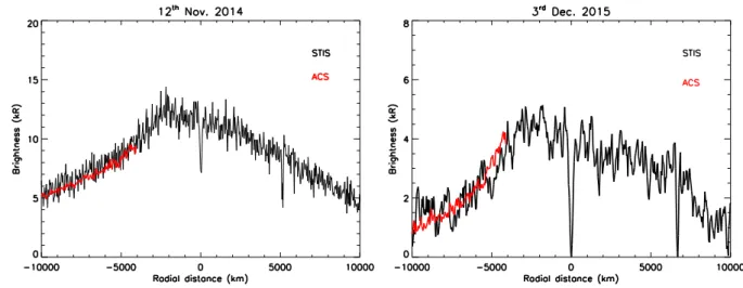
The new calibration factor derived for ACS was tested by comparing overlapping 467
observations of the martian hydrogen Lyman α emission obtained using STIS and ACS on 12th
468
November 2014 and 3rd December 2015. Figure 3b shows the comparison between the STIS and
469
the ACS intensity of the martian exosphere at 1215.67 Å. The two profiles lie on top of each other 470
for both the observing visits thereby validating the new ACS calibration factor. 471
472
Figure 3a: This figure shows the geocoronal intensities observed by the STIS instrument as well
473
as the ACS instrument onboard HST when observing the same patch of the sky with HST’s orbital
474
position in degrees. The ACS intensities processed using the old calibration factor (0.002633
counts pixel-1 sec-1 kR-1) do not match up well with the STIS intensities, whereas, with the new 476
calibration factor the values recorded by the two instruments overlap completely.
477
478
Figure 3b: The above two figures show the brightness of Mars’ Lyman α emission (with the
479
geocoronal + interplanetary hydrogen background subtracted) as observed by STIS (black) and
480
ACS (red) on 12th November, 2014 and 3rd December, 2015. The new calibration factor derived 481
for ACS was used to determine the brightness of the martian hydrogen exosphere as observed by
482
ACS for the above two observations. As can be seen in the two figures, the ACS intensities match
483
those measured by STIS, i.e. the red line (ACS intensity) overlaps with the black line (STIS
484
intensity) for both observations.
485
Comparison of HST-ACS observed brightness for the martian exosphere with MAVEN is 486
not a straightforward process. The two instruments have different observing geometry and lines of 487
sight. The ACS brightness values have to be analyzed and fit to models to obtain the hydrogen 488
density distribution in the martian exosphere that best matches the data for a particular day of 489
observation. Using this density distribution, the modeled HST brightness for MAVEN-IUVS 490
observing geometry can then be derived and compared with the actual brightness recorded by the 491
MAVEN satellite in orbit around Mars on the same observation date. This comparison study was 492
conducted for two specific dates, 12th November 2014 and 3rd December 2015 where there were
493
corresponding dayside observations available with both HST and MAVEN. For the comparison 494
study, only disk observations of Mars by the MAVEN-IUVS echelle were used in order to avoid 495
uncertainties in the modeling process brought on by the presence of interplanetary hydrogen 496
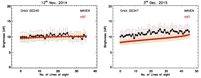
background in the MAVEN-IUVS signal. Figure 4 shows the comparison between the model 497
derived brightness that would be observed by HST (red points) in MAVEN’s observing geometry 498
with the actual brightness observed by MAVEN-IUVS echelle (black points). The brightness 499
derived from modeling the HST observations and the actual brightness observed by MAVEN are 500
within the uncertainty. There is an offset between HST and MAVEN intensities for the 2015 501
observations which could be due to an inaccurate derivation of Mars’ exospheric characteristics 502
from the HST observations because of larger noise in the data (Figure 7) as a result of low count 503
rate since Mars was close aphelion during the 2015 observation with the solar activity approaching 504
minimum. However, the MAVEN IUVS observational intensities for 3rd December 2015 do fall
505
within the 10% uncertainty accorded to the model results. 506
A similar comparison study was presented in Mayyasi et al. [2017a] for the 12th November
507
2014 overlapping observations with MAVEN-IUVS echelle and HST. However, the HST 508
observations were reduced using the old calibration factor for ACS and the modeling was done 509
using a 1-dimensional radiative transfer model for observed H Lyman α intensities. The resulting 510
comparison with MAVEN was not as accurate as the figure below [figure 4 left]. 511
512
Figure 4: Comparison between the model derived Mars disk brightness that would be observed
513
by HST (red points) in MAVEN-IUVS echelle observing geometry with the actual brightness
514
observed by MAVEN-IUVS Echelle (black points) on 12th November 2014 and 3rd December 2015. 515
The uncertainty in the brightness observed by MAVEN due to the ~25% uncertainty in absolute
516
calibration is represented by the light pink lines whereas the light green lines represent the
517
uncertainty in the model derived brightness which is taken to be ~10%.
518
4.2 Modeling MAVEN and HST observations using an asymmetric atmosphere
MAVEN observations of H and D Lyman α as well as HST observations of H Lyman α were 520
modeled using an asymmetric atmosphere and the 2-D radiative transfer model as described in 521
sections 2 and 3 respectively. The MAVEN observations with the IUVS-echelle instrument are 522
restricted to lower tangent altitude ranges between 0 – 300 km, whereas the HST observations 523
extend from 700 – 30,000 km. The hydrogen exosphere at Mars approaches a more uniform and 524
spherically symmetric structure above ~2.5 martian radii [Holmström, 2006; Bhattacharyya et al., 525
2017a]. Therefore, the 2-D model is more important for an accurate analysis and interpretation of 526
the MAVEN IUVS-echelle observations of the martian H Lyman α emission. 527
4.2.1. Modeling MAVEN IUVS-Echelle Observations of Deuterium
528
MAVEN IUVS-Echelle observations of D Lyman α between November 2014 – October 2017 have 529
been analyzed using the 2-D asymmetric model in order to derive best-fit exobase densities for D 530
(2952 orbits in total), the results of which have been published in Mayyasi et al. [2019]. These 531
observations have also been previously used to study the seasonal variability of the deuterium 532
Lyman α intensity in the martian exosphere [Clarke et al., 2017; Mayyasi et al., 2017]. In this 533
paper, a detailed description of the modeling process supporting the data analysis is presented. 534
For modeling the MAVEN IUVS-Echelle observations of D, first the exobase temperatures are 535
pre-determined by interpolating NGIMS observations at aphelion and perihelion for all the 536
MAVEN-IUVS echelle orbits (section 2.1). Then the 2-D atmosphere model was used to produce 537
density distributions for a total of 7 different exobase densities, 100, 500, 1000, 3000, 5000, and 538
7000 cm-3 at SZA of 0° for every MAVEN IUVS echelle orbit (2952 × 7 = 20664 atmospheres
539
simulated). For each model atmosphere corresponding to a particular MAVEN IUVS echelle orbit, 540
the line of sight deuterium Lyman α intensity was calculated by deriving the column density along 541
that line of sight and multiplying it by the excitation frequency of Lyman α at 1215.33 Å (eq.6). 542
The line integrated solar Lyman α at 1215.67 Å flux is measured by the Extreme Ultraviolet 543
Monitor (EUVM) instrument onboard the MAVEN orbiter at Mars [Eparvier et al., 2015]. It has a 544
full width half max (FWHM) of 1Å and therefore encompasses the solar Lyman α flux at 1215.33 545
Å. From the EUVM measurements of the line integrated flux, the Lyman α flux at line center 546
(1215.67 Å) was calculated by using the widely-used Emerich relationship [Emerich et al., 2005]. 547
Based on the shape of the Lyman α profile, the solar Lyman α flux at 1215.33 Å is derived, which 548
is almost the same as the flux at line center (greater by ~1.6%), and this value is used in determining 549
the excitation frequency of Lyman α at 1215.33 Å for all the MAVEN-IUVS echelle orbits. 550
Since the deuterium signal is faint at Mars, the data was binned into Ls, SZA and altitude bins
551
to obtain intensity profiles with altitude for deuterium. Six Ls bins were created with 20° spacing
552
within solar longitudes 220° - 340°, four SZA bins were created between 30° - 90° with 15° spacing 553
and twenty one altitude bins were created between 0 – 400 km with 20 km spacing as elaborated 554
in Mayyasi et al., [2019]. The model followed the same binning scheme as the data using the 2952 555
orbits to produce simulated intensity profiles with altitude which can then be compared to the data. 556
These modeled intensity profiles derived for the seven different exobase densities were then 557
linearly interpolated on a more refined exospheric density grid to obtain the best fit exospheric 558
density of deuterium that matched the data through the process of c2 minimization.
559
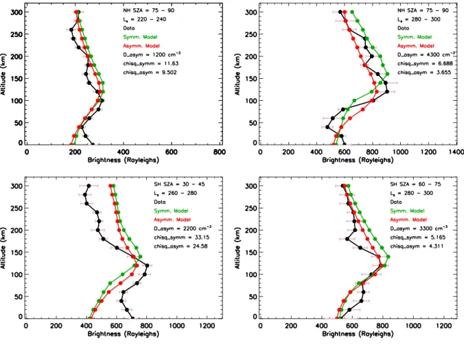
Figure 5 shows the comparison between the best fit modeled density to the data for deuterium 560
as measured by IUVS echelle using the spherically symmetric model, which assumes an isothermal 561
symmetric atmosphere [Bhattacharyya et al., 2017a], and the spherically asymmetric model 562
described here. The figure shows four cases for available dayside solar zenith angles for the 563
northern hemisphere (top two plots) and the southern hemisphere (bottom two plots) as observed 564
by the IUVS echelle instrument onboard MAVEN [Mayyasi et al., 2019]. In all cases the 565
asymmetric model fits the data better than the symmetric model for the exobase density displayed 566
in the respective figures. However, even the asymmetric model fails to provide perfect fits to the 567
data, especially at lower altitudes. This is because the D signal is above the detection threshold of 568
the MAVEN-IUVS detector only between Ls = 220° - 340° and the dataset presented in figure 5,
569
which was analyzed and reported in Mayyasi et al. [2019], has dayside coverage of that solar 570
longitude range only during late 2014 – early 2015. During this time MAVEN had just started its 571
science phase and the optimal conditions like detector gain, binning scheme, observing geometry, 572
etc. for recording the D emission from the martian exosphere had not yet been established, thereby 573
degrading the quality of the data collected. It is expected that more IUVS observations of the D 574
emissions through multiple perihelion passages of Mars in the future would provide better model 575
fits to the data. 576
An advantage of the asymmetric model is that it allows analysis and comparison of IUVS 577
observations at different solar zenith angles under the same solar longitude and solar activity 578
conditions using a single model run in order to better constrain the asymmetric nature of Mars’ 579
exosphere. Presently, this has not been possible for D due to the lack of observations [Mayyasi et 580
al., 2019]. But with IUVS’s continued observations of the D Lyman α emission with every 581
perihelion passage of Mars, this would soon be possible. 582
583
Figure 5: This figure displays the symmetric and asymmetric model fits to the IUVS-Echelle
584
deuterium observation for a predetermined exobase temperature from MAVEN-NGIMS
585
observations and an exobase density at SZA = 0° as displayed in the figures. The exobase density
586
varied with SZA following the Hodges and Johnson [1968] formulation for the asymmetric model,
587
but remained constant for the symmetric model. The top two plots are for the northern hemisphere
588
and the bottom two plots are for the southern hemisphere. These simulations are for an
MAVEN-589
NGIMS measured aphelion temperature of 216 K and a perihelion temperature of 255 K [Mayyasi
590
et al., 2019].
591
4.2.2. Modeling MAVEN IUVS-Echelle Observations of Hydrogen
MAVEN observations of H Lyman α between November 2014 – October 2017, simultaneously 593
observed with the D Lyman α emission by the IUVS echelle instrument, have been utilized in this 594
study (2952 orbits in total). Some of the observations have been previously used to study the 595
seasonal variability of hydrogen in the martian exosphere as well as the response of the H escape 596
rate to solar flare events [Clarke et al., 2017; Mayyasi et al., 2018]. For modeling the MAVEN 597
observations of hydrogen, the 2-D radiative transfer model (Appendix B) in conjunction with the 598
2-D atmosphere model (section 2; Appendix A) was used to determine the emissivity for a range 599
of exobase densities for thermal hydrogen (104 – 7 × 105 cm-3; 13 different exobase density values)
600
at Mars’ aphelion and perihelion positions (26 simulations with the 2-D atmosphere + RT model). 601
The exobase temperatures at perihelion and aphelion positions were pre-determined by averaging 602
NGIMS observations of the lower thermosphere conducted over a period of ~1.5 Mars years 603
(section 2). The emissivity of Mars’ atmosphere for all the MAVEN-IUVS echelle orbits (2952 604
orbits in total) for each exobase was calculated by sinusoidally interpolating the emissivity 605
determined at aphelion and perihelion using the 2-D RT model using eq. 1. The Lyman α line 606
center flux at 1215.67 Å in the model was determined from EUVM measurements of the line 607
integrated flux which were then converted to line center flux using Emerich’s analytical formula 608
[Emerich et al., 2005]. Next, the line of sight hydrogen Lyman α intensity for each MAVEN-IUVS 609
echelle orbit was calculated using equation 7. The model results were then binned into solar 610
longitudes, SZA and altitude bins, same as the deuterium observations to facilitate D/H 611
calculations which will be published in a future study. This modeled and observed intensity 612
profiles were compared and the density that best matched the data was determined through the 613
process of c2 minimization. Non-thermal hydrogen was not considered in the modeling process
614
because the altitude profiles are restricted to line of sight altitudes below ~3000 km, where the 615
thermal component is dominant. 616
Figure 6 shows the comparison between MAVEN IUVS echelle measurements of H Lyman α 617
emission and the best modeled fit to the data using the asymmetric model and the symmetric 618
model. This figure displays the corresponding H Lyman α emission to the D Lyman α emission 619
measured by the IUVS echelle instrument displayed in figure 5. The error bars are larger for the 620
fainter D Lyman α emission than for the much brighter and easily detectable H Lyman α emission. 621
Unlike the D observations, the H Lyman α observations above the limb include a contribution from 622
the interplanetary hydrogen (IPH). The IPH intensity was estimated using the widely used Pryor 623
model [Pryor et al., 1992; 2013; Ajello et al., 1987]. As is evident from the figure, the asymmetric 624
model provides a better fit to the data than the symmetric model for the exobase density displayed 625
in the respective figures. 626
627
Figure 6: This figure displays the symmetric and asymmetric model fits to the IUVS-Echelle
628
hydrogen observations for a predetermined exobase temperature from MAVEN-NGIMS
629
observations and an exobase density at SZA = 0° as displayed in the figures. The exobase density
630
varied with SZA following the Hodges and Johnson [1968] formulation for the asymmetric model,
631
but remained constant for the symmetric model. The top two plots are for the northern hemisphere
632
and the bottom two plots are for the southern hemisphere. These simulations are for an
MAVEN-633
NGIMS measured aphelion temperature of 216 K and a perihelion temperature of 255 K [Mayyasi
634
et al., 2019].
635
4.2.3. Modeling HST Observations of Hydrogen
Two sets of HST observations obtained on 12th November 2014 and 3rd December 2015 were
637
modeled using the 2-D atmosphere + radiative transfer model as well as the 1-D atmosphere + 638
radiative transfer model and the comparison between the two model results were studied. On the 639
above-mentioned observation dates, Mars was imaged using two different instruments on the HST, 640
i.e., ACS and STIS. The ACS instrument was used to image the highly extended dayside hydrogen 641
exosphere of Mars. The ACS images for the martian Lyman α emission are a difference between 642
two images obtained with the F115LP filter, which transmits Lyman α, and the F140LP filter, 643
which blocks Lyman α but allows emissions up to 140 nm wavelengths. Therefore, the disk of 644
Mars in the final differenced image is noisy on account of other emissions like oxygen 130.4 nm 645
and the 135.6 nm emissions and solar continuum. However, above ~700 km the hydrogen Lyman 646
α emission becomes dominant. Therefore, the ACS observations capture the Mars H Lyman α 647
profile accurately above ~700 km. The STIS observations, on the other hand, can spectrally isolate 648
the Lyman α emission from the Mars disk. Thus, both ACS and STIS observations of Mars were 649
combined together to obtain the martian H Lyman α intensity profile from the dayside to the night 650
side including the disk. Background emissions from the interplanetary hydrogen (IPH) and the 651
geocorona in the Mars observations were estimated using a dedicated HST orbit as a part of each 652
visit which observed the background blank sky 5 arcminutes away from Mars for the same portion 653
of HST’s orbit as the Mars observations with STIS and ACS. The estimated background intensity 654
was then subtracted off from the Mars H Lyman α data. Figure 7 shows the final Mars H Lyman 655
α profile obtained for the two observation days. 656
Figure 7: Asymmetric and symmetric model fits to HST observations of the martian exospheric
658
hydrogen Lyman α emission observed on 12th November 2014 and 3rd December 2015. The data 659
consists of dayside exospheric observations with the ACS instrument along with the martian disk
660
and night side observations with the STIS instrument onboard HST. The asymmetric model fits the
661
disk and the night side intensities better than the symmetric model. The differences between the
662
asymmetric and the symmetric model intensities become small above ~2.5 martian radii suggesting
663
that the martian hydrogen exosphere approaches symmetry at higher altitudes.
664
For modeling the HST observations using the 2-D RT model, first the 2-D density model 665
was used to generate density profiles with thermal hydrogen exobase densities at SZA = 0° ranging 666
from 1 × 104 cm-3 – 5 × 105 cm-3 (11 different density values). The exobase temperature at SZA =
667
0° for the two observation days were taken from the Mars Global Circulation Model (MGCM) 668
[Chaufray et al., 2015; 2018]. MAVEN-NGIMS observations were not used here because 669
MAVEN’s orbit on these days did not sample close to the sub-solar point. The 2-D RT model was 670
then used to simulate the emissivity of the atmosphere for each exobase density. The thermal H 671
density that best matches the STIS observation up to ~2000 km through least-squares minimization 672
was used to determine the thermal H population for that particular HST observation. The 673
superthermal population of H atoms was determined through the same method as used in previous 674
HST observation analysis [Bhattacharyya et al. 2015; 2017a; 2017b]. The temperature of the H 675
superthermal population was taken to be 800 K. Different exobase densities for superthermal H 676
ranging from 1 × 103 cm-3 – 4 × 104 cm-3 were added to the best-fit thermal density profile and the
677
emissivity of the atmosphere was then determined using the 2-D RT model. The density of the 678
superthermal population of H was not varied with SZA. The best-fit non-thermal density was then 679
determined through chi-square minimization of the model fits to the ACS intensity profile, which 680
extends from ~700 km to ~30,000 km and contains emissions from superthermal H atoms which 681
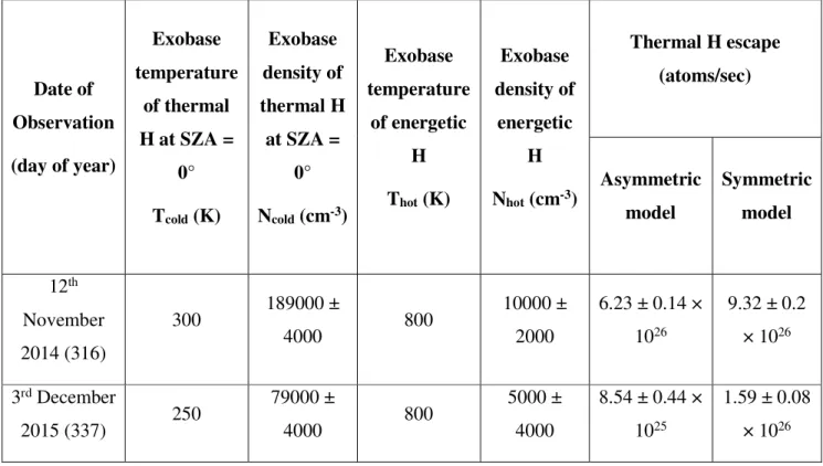
become significant at higher altitudes (above ~20,000 km). Table 1 lists the best-fit thermal and 682
superthermal H densities and temperatures for the two HST observation days. These values were 683
then used in a symmetric 1-D model where the temperature and density varied only radially and 684
not with SZA to simulate the intensity from a spherically symmetric and isothermal atmosphere. 685
Figure 7 shows the comparison between the output from the symmetric and the asymmetric model 686
for both the 12th November 2014 observation as well as the 3rd December 2015 observation of the
687
martian hydrogen Lyman α emission HST. As is evident from the figure, the asymmetric model 688
fits the data better than the symmetric model, especially the disk brightness and the night side 689
brightness for the martian H corona. However, differences between the symmetric and the 690
asymmetric model intensities decrease above an altitude of ~2.5 martian radii as the martian 691
hydrogen exosphere approaches symmetry in conjunction with previous studies [Holmström, 692
2006; Bhattacharyya et al., 2017a; Chaufray et al., 2015]. The Jeans escape flux derived from the 693
symmetric model fits are greater than the asymmetric model fits to the data by a factor of 1.5 and 694
1.87 for the two HST observations. 695
Table 1: Modeled characteristics of the hydrogen exosphere for the HST observations
696 Date of Observation (day of year) Exobase temperature of thermal H at SZA = 0° Tcold (K) Exobase density of thermal H at SZA = 0° Ncold (cm-3) Exobase temperature of energetic H Thot (K) Exobase density of energetic H Nhot (cm-3) Thermal H escape (atoms/sec) Asymmetric model Symmetric model 12th November 2014 (316) 300 189000 ± 4000 800 10000 ± 2000 6.23 ± 0.14 × 1026 9.32 ± 0.2 × 1026 3rd December 2015 (337) 250 79000 ± 4000 800 5000 ± 4000 8.54 ± 0.44 × 1025 1.59 ± 0.08 × 1026 697
5. Summary and Discussion
698
Observations and analysis of the martian exospheric Lyman α emission in the past decade have 699
slowly revealed the complicated nature of this tenuous upper atmospheric layer. The presence of 700
a superthermal H component have been inferred from the analysis of Mars Express (MEX), HST 701
and MAVEN observations [Chaufray et al., 2008; Chaffin et al., 2014; 2015; Clarke et al., 2014; 702
Bhattacharyya et al., 2015]. These observations also revealed that the exosphere is not spherically 703
symmetric and isothermal [Holmström, 2006; Chaffin et al., 2015; Bhattacharyya et al., 2017a]. 704
MAVEN-NGIMS observations of the lower thermosphere reported temperature differences of > 705
100 K between the day and the night side indicating a non-isothermal exosphere [Stone et al., 706
2018] and models imply a large difference in H density between subsolar and anti-solar point 707
[Chaufray et al., 2018]. Therefore, in this study a more physically accurate 2-dimensional model 708
of the martian exosphere based on MAVEN findings was constructed which would provide better 709
constraints on the present-day escape rates of deuterium and hydrogen atoms from the exosphere 710
of Mars. It is imperative to obtain an accurate value for the escape rate of H as it is tied to the 711
escape of water from Mars, whereas an accurate estimate of the D/H ratio will help establish the 712
timeline for the escape of the martian atmosphere throughout its history of evolution. 713
Uncertainties in estimating the D and H escape rate arise from both uncertainties in the 714
data as well as the modeling process as was concluded from the Bhattacharyya et al. [2017] study. 715
The data uncertainties are mostly dominated by the uncertainty in the instrumental absolute 716
calibration [Bhattacharyya et al., 2017a]. A recent HST observation campaign utilized the STIS 717
instrument onboard HST, whose absolute calibration is well-documented (within 5%) through 718
observations of standard UV stellar sources, to determine the sensitivity of the ACS instrument at 719
Lyman α. The ACS instrument, which is a broadband filter, has been used to image the H Lyman 720
α emission from many different planetary hydrogen coronae, including Mars. Therefore, 721
calibrating the ACS detector at Lyman α will help reduce the uncertainties associated with 722
determining the H escape rate from Mars through analysis of HST ACS observations. The 723
MAVEN-IUVS echelle Lyman α calibration factor was cross-checked with overlapping HST 724
observations. However, the observed martian H Lyman α intensity by the MAVEN-IUVS echelle 725
cannot be directly compared to the intensities recorded by HST due to the differences in their 726
observing geometry. A 2-D radiative transfer model was utilized to obtain the characteristics of 727
the martian hydrogen exosphere (hydrogen exobase density and temperature) for a particular day 728
of observation (12th November 2014 and 3rd December 2015). This “best-fit” atmosphere for that
729
particular day of observation was then used to simulate the H Lyman α intensities that would be 730
observed by HST from the MAVEN-IUVS echelle observing geometry on that day. Assuming a 731
10% uncertainty in the modeling process, the MAVEN observed intensity, with its present 732
calibration factor (including a 25% uncertainty), lies within the HST simulated intensity limits. 733
Model uncertainties are a result of the various assumptions made in the simulation process 734
about the characteristics of the martian exosphere. Earlier models assumed a spherically symmetric 735