HAL Id: cea-01135423
https://hal-cea.archives-ouvertes.fr/cea-01135423
Submitted on 25 Mar 2015
HAL is a multi-disciplinary open access
archive for the deposit and dissemination of
sci-entific research documents, whether they are
pub-lished or not. The documents may come from
teaching and research institutions in France or
abroad, or from public or private research centers.
L’archive ouverte pluridisciplinaire HAL, est
destinée au dépôt et à la diffusion de documents
scientifiques de niveau recherche, publiés ou non,
émanant des établissements d’enseignement et de
recherche français ou étrangers, des laboratoires
publics ou privés.
On preferred axes in WMAP cosmic microwave
background data after subtraction of the integrated
Sachs-Wolfe effect
A. Rassat, J.-L. Starck
To cite this version:
A. Rassat, J.-L. Starck. On preferred axes in WMAP cosmic microwave background data after
sub-traction of the integrated Sachs-Wolfe effect. Astronomy and Astrophysics - A&A, EDP Sciences,
2013, 557, pp.L1. �10.1051/0004-6361/201321537�. �cea-01135423�
DOI:10.1051/0004-6361/201321537
c
ESO 2013
Astrophysics
&
L E
On preferred axes in WMAP cosmic microwave background data
after subtraction of the integrated Sachs-Wolfe effect
?,??
A. Rassat
1,2and J.-L. Starck
21 Laboratoire d’Astrophysique, École Polytechnique Fédérale de Lausanne (EPFL), Observatoire de Sauverny, 1290 Versoix,
Switzerland
e-mail: [email protected]
2 Laboratoire AIM, UMR CEA-CNRS-Paris, Irfu, SAp, CEA Saclay, 91191 Gif-sur-Yvette Cedex, France
Received 21 March 2013/ Accepted 25 May 2013
ABSTRACT
There is currently a debate over the existence of claimed statistical anomalies in the cosmic microwave background (CMB), recently confirmed in Planck data. Recent work has focussed on methods for measuring statistical significance, on masks and on secondary anisotropies as potential causes of the anomalies. We investigate simultaneously the method for accounting for masked regions and the foreground integrated Sachs-Wolfe (ISW) signal. We search for trends in different years of WMAP CMB data with different mask treatments. We reconstruct the ISW field due to the 2 Micron All-Sky Survey (2MASS) and the NRAO VLA Sky Survey (NVSS) up to `= 5, and we focus on the Axis of Evil (AoE) statistic and even/odd mirror parity, both of which search for preferred axes in the Universe. We find that removing the ISW reduces the significance of these anomalies in WMAP data, though this does not exclude the possibility of exotic physics. In the spirit of reproducible research, all reconstructed maps and codes will be made available for download athttp://www.cosmostat.org/anomaliesCMB.html.
Key words.cosmic background radiation – cosmology: observations – early Universe – large-scale structure of Universe – cosmology: theory – dark energy
1. Introduction
In recent years, several violations of statistical isotropy have been reported on the largest scales of the cosmic microwave background (CMB). A low quadrupole was reported in COBE data (Hinshaw et al. 1996; Bond et al. 1998) and confirmed later with WMAP data (Spergel et al. 2003; Gruppuso et al. 2013). The octopole presented an unusual planarity and its phase seemed correlated with that of the quadrupole (Tegmark et al. 2003;de Oliveira-Costa et al. 2004;Slosar & Seljak 2004;Copi et al. 2010). Other anomalies include a north/south power asym-metry (Eriksen et al. 2004;Bernui et al. 2006), an anomalous cold spot (Vielva et al. 2004; Cruz et al. 2005, 2006), align-ments of other large-scale multipoles (Schwarz et al. 2004;Copi et al. 2006), the so-called “Axis of Evil” (AoE,Land & Magueijo 2005a) and other violations of statistical isotropy (Hajian & Souradeep 2003; Land & Magueijo 2005b). Recently, Planck has confirmed that these large-scale anomalies are still present in the CMB (Planck Collaboration 2013a,b), ruling out any ori-gin due to a systematic in the data.
These anomalies are interesting because they point towards a possible violation of the standard model of cosmology, which predicts statistical isotropy and Gaussian fluctuations in the CMB, and therefore offer a window into exotic early-universe
? Appendices are available in electronic form at http://www.aanda.org
??
Reconstructed maps and codes are only available at the CDS via anonymous ftp tocdsarc.u-strasbg.fr(130.79.128.5) or via
http://cdsarc.u-strasbg.fr/viz-bin/qcat?J/A+A/557/L1
physics (e.g., Liu et al. 2013a,b; Wang 2013; Buckley & Schlegel 2013). However, there is still much debate over the possible causes of these anomalies. Since these effects are on very large scales where there is large cosmic variance, the statis-tics used to measure the significance of the anomalies are sub-tle (Bennett et al. 2011;Efstathiou et al. 2010;Gold et al. 2011; Hinshaw et al. 2012). They could also be due to some foreground effects, which could be either contamination due to Galactic foreground effects (Hinshaw et al. 2012;Kim et al. 2012) or cos-mological foregrounds that lead to secondary anisotropies in the CMB (Rassat et al. 2007;Rudnick et al. 2007;Peiris & Smith 2010;Smith & Huterer 2010; Yershov et al. 2012; Francis & Peacock 2010;Rassat et al. 2013).
Rassat et al. (2013) have simultaneously investigated the impact of masks and the integrated Sachs-Wolfe (ISW) effect. Missing data were accounted for with the sparse inpainting tech-nique described inStarck et al.(2013b), which does not assume the underlying field is either Gaussian or isotropic, but allows for it to be. It was found that removing the ISW reduced the signifi-cance of two anomalies in WMAP data (the quadrupole/octopole alignment and the octopole planarity). In this work we focus on two anomalies, both related to preferred axes on the sky: the AoE effect and mirror parity. In Sect.2we describe the reconstruc-tion of the ISW field from 2MASS and NVSS data. In Sect.3, we search for violations of statistical isotropy before and after inpainting, as well as after both inpainting and ISW subtraction. In Sect.4we discuss our results and summarise our results com-pared with those fromRassat et al.(2013).
A&A 557, L1 (2013) 2. Estimating the large-scale primordial CMB
2.1. Theory
Since statistical isotropy is predicted for the early Universe, analyses should focus on the primordial CMB, i.e. one from which secondary low-redshift cosmological signals have been removed. In AppendixD, we briefly review how to estimate the primordial CMB with a reconstructed map of the ISW effect. In practice, we estimate the primordial CMB on large scales by
ˆ
δprim'δOBS− ˆδ2MASSISW − ˆδ NVSS
ISW −δkD,` = 2, (1)
where ˆδ2MASSISW and ˆδNVSSISW are the estimated ISW contributions from the 2MASS and NVSS surveys (see Sect.2.2, AppendixD and Sect. 2.2 from Rassat et al. 2013, for details on how these are estimated). The terms δOBS and δprimcorrespond to the
ob-served and primordial CMB respectively. The term δkD,` = 2is the
temperature signal due to the kinetic Doppler quadrupole (Copi et al. 2006;Francis & Peacock 2010), for which we have pro-duced publicly available maps inRassat et al.(2013).
2.2. Data
We are interested in identifying trends and therefore considered WMAP renditions from various years, both before and after in-painting. These maps are described in Table 1 of Rassat et al. (2013, see also Appendix A). The 2MASS (Jarrett 2004) and NVSS (Condon et al. 1998) data sets are described in Sects. 3.2 and 3.3 or inRassat et al.(2013).
We use the reconstructed ISW effect due to 2MASS and NVSS galaxies, using the method in Dupé et al. (2011) and Rassat et al. (2013), but reconstructing the ISW fields up to ` = 5. The ISW reconstruction method is cosmology indepen-dent, and estimates the ISW amplitude directly from the CMB and galaxy field cross-correlations. This means that there is a different ISW map for each CMB map rendition considered. All map reconstructions are done using the publicly available ISAP code, and the specific options used are described in detail inRassat et al.(2013).
The large-scale ISW temperature field (` = 2−5) due to 2MASS and NVSS (where the amplitude is estimated from a correlation with WMAP9 data) is plotted in Fig.1. Since there is little redshift overlap between the surveys (see Fig. 3 inRassat et al. 2013), we estimate the ISW contribution from each survey independently and add the two resulting ISW maps to produce the map in Fig.1.
In Fig. 2, we plot the amplitude of the ISW temperature power CISW
TT (`) for ` = 2 − 5, which is measured directly from
the map plotted in Fig.1, showing the theoretical prediction for a “Vanilla-model” cosmology and taking contributions into ac-count from both 2MASS and NVSS galaxies. Data points are shown for WMAP9, 2MASS, and NVSS data with Gaussian er-rors bars estimated analytically and assuming fskyNVSS= 0.66 (i.e. the smallest fsky value amongst the three maps). In general, we
find that the ISW signal is below what is expected from theory for the fiducial cosmology we assumed.
3. Preferred axes in WMAP data before and after inpainting and ISW subtraction
We focus on both the AoE statistic and the even/odd mirror par-ity anomalies, which are described in detail in Appendix B. In
Fig. 1.Large-scale ISW temperature field (` = 2−5) due to 2MASS and NVSS galaxies. The amplitude is estimated directly from the data, including cross-correlation with WMAP9 data.
Fig. 2. Amplitude of the ISW temperature power CISW
TT (`) (in µK 2)
for ` = 2−5. The solid line is the theoretical prediction, and the data points are estimated from 2MASS and NVSS galaxies with WMAP9 data are shown with Gaussian error bars assuming fsky= 0.66,
i.e. the sky coverage of the NVSS survey.
AppendixC, we validate that sparse inpainting provides a bias-free reconstruction with which to study these anomalies using a large set of simulated CMB maps.
3.1. Axis of Evil (AoE)
Rassat et al.(2007) searched for an AoE directly in 2MASS data, hoping that this could link the measured anomaly to the ISW ef-fect, but found no preferred axes in 2MASS data. Here, we can test an estimate of the primordial CMB estimated directly.
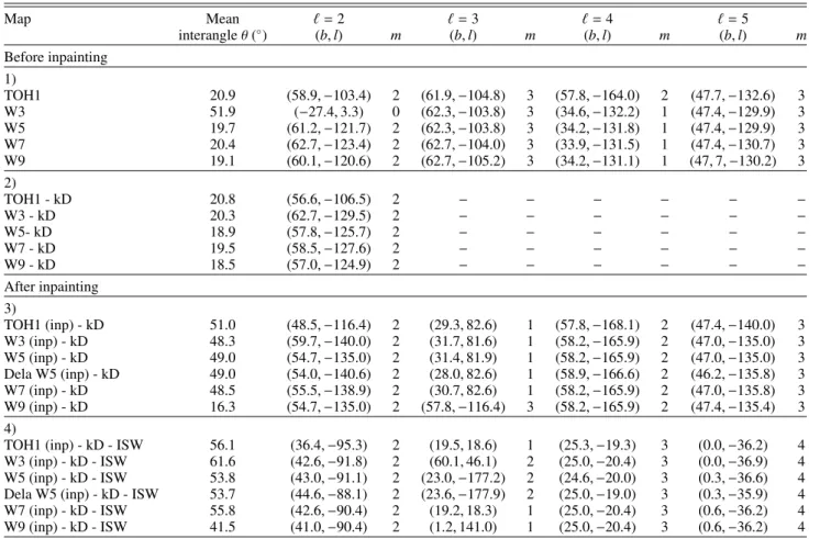
In Table D.1 we report the preferred modes and axes for the 11 CMB maps considered in this paper. This table can be di-rectly compared with Table 1 inLand & Magueijo(2007), which reviewed the preferred modes and axes for W1 and W3 data. By analysing the “raw” maps (Sect. 1 of Table D.1), we confirm their result that the preferred axis that was present in first-year data is not present in the ILC W3 data. We find the mean interan-gle is anomalously low for 4 WMAP renditions (TOH1, W5, W7, W9) with θ ∼ 20◦, but that for W3 data, θ ∼ 52◦, similar to whatLand & Magueijo(2007) found for W1 and W3 maps in their updated analysis of the AoE. As they found, the change occurs because the preferred mode for ` = 2 is m = 2 for W1 (and also years 5 to 9), whereas for W3 data, the preferred mode
for ` = 2 is m = 0. They attribute this fact to the discontinuous nature of the AoE statistic, and underline how this feature con-stitutes a weakness in the AoE statistic.
However, followingFrancis & Peacock(2010), we subtract the kinetic Doppler (kD) from the public WMAP maps (i.e. by subtracting the last term in Eq. (1)) and re-perform the AoE anal-ysis (Sect. 2 of Table D.1, where only the quadrupole ` = 2 has changed). We find the statistic is now stable across all WMAP data considered, with the mean interangle spanning θ= 18.5−20.8◦.
The results after inpainting of the CMB maps (and kD sub-traction) are presented in Sect. 3 of TableD.1. We find inpaint-ing has no effect on the preferred modes and directions for ` = 2 and ` = 5, which are generally unchanged and are the same for all maps, as was the case before inpainting. For ` = 4, the preferred mode and direction for all WMAP renditions now be-comes similar to that for the TOH map before inpainting. The oc-topole (`= 3) is the scale that changes the most after inpainting, both preferred mode and direction are changed for all WMAP renditions. The preferred modes and directions for ` = 2−5 are quite stable across all WMAP renditions after inpainting. We note that when searching for quadrupole/octopole alignment, Rassat et al. (2013) showed that the preferred axis of the oc-topole was stable after inpainting. However, this statistic en-forced a search within a planar mode (m = 3), which explains the difference in stability for the octopole.
The change of only one preferred mode, notably the octopole in the W9 rendition that prefers the planar mode m = 3 rather than m= 1 for other WMAP renditions, has a significant effect on the mean interangle θ that changes from 48.3−51.0◦for
W1-7 data to 16.3◦, a value which is only found in 0.1% of simula-tions. Further studies with improved (and smaller) masks, either on WMAP or Planck data, could point to why the AoE statistic on W9 data is so different.
The results after inpainting and ISW subtraction are pre-sented in Sect. 4 of TableD.1. For the quadrupole, the preferred mode remains the same, and the preferred direction changes slightly. The scale with the most change are `= 3−5, where both preferred mode and direction change for all WMAP renditions. In general, there is very good agreement across different WMAP renditions, except some differences for the octopole. After in-painting and ISW subtraction, the mean interangle now varies between 41.5◦−61.6◦, which corresponds to 5.8−61.5% of val-ues found in simulations. Even for the lowest value of 5.8%, the original anomalous alignment is no longer as significant as the previous value of 0.1% on the ILC maps.
3.2. Parity
We calculate the S±values for each of the WMAP renditions
using Eq. (B.3), and results are presented in TableD.2, where the significance is calculated using 1000 full-sky Gaussian re-alisations. Before inpainting (part 1 of TableD.2), we find no significant even (S+) or odd (S−) mirror parity, except for the
TOH map, which shows a mild preference for even mirror parity (only 2.6% of simulations have a higher S+value). After sparse inpainting (part 2 of Table D.2), we find an increase in both even and odd mirror parity anomalies (except for the TOH map), with only 3.2−3.6% of the simulations having a higher value for S−than both W7 and W9 maps and only 0.90−3.1% of the
simulations having a higher value for S+. The significance of these remains at <3σ though. We find the mirror-parity anoma-lies do not persist after sparse inpainting and subtraction of the
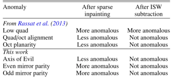
Table 1. Summary of results in this paper andRassat et al.(2013).
Anomaly After sparse After ISW
inpainting subtraction FromRassat et al.(2013)
Low quad More anomalous More anomalous
Quad/oct alignment Less anomalous Not anomalous Oct planarity Less anomalous Not anomalous This work
Axis of Evil Less anomalous Not anomalous
Even mirror parity More anomalous Not anomalous Odd mirror parity More anomalous Not anomalous Notes. The anomalies in WMAP could be explained by the ISW effect, though other explanations remain possible.
reconstructed ISW signal (part 3 of TableD.2), meaning the ISW could explain these anomalies.
4. Discussion
One of the main successes of the standard model of cosmology is its prediction of the Gaussian random fluctuations observed in the CMB. However, even since COBE data, several signatures of lack of statistic isotropy, or “anomalies”, have been reported on large scales in WMAP data and recently confirmed in Planck data (Planck Collaboration 2013a,b). Recent focus has been on testing the impact of different reconstruction methods or meth-ods for dealing with Galactic foregrounds, while others have in-vestigated how various foreground cosmological signals could affect these anomalies.
In Rassat et al.(2013), we found that subtracting the ISW signal due to 2MASS and NVSS data from WMAP data low-ered the significance of two previously reported anomalies: the quadrupole/octopole alignment and the octopole planarity.
In this work, we continued investigation of two other anoma-lies, both related to preferred axes in the sky: the Axis of Evil (AoE) and even/odd mirror parity in CMB data, i.e. parity with respect to reflections through a plane. We first investigated whether sparse inpainting can be considered a bias-free recon-struction method for the two statistics and found that this is the case. We then applied sparse inpainting on various CMB maps up to `= 5 and reconstructed the ISW maps from 2MASS and NVSS data also up to `= 5. We considered the significance of the two reported anomalies, before inpainting, after inpainting, and both after inpainting and ISW subtraction.
Our first approach to the AoE was to remove the kD quadrupole (followingFrancis & Peacock 2010), and we found that the AoE is consistent across all renditions of WMAP data (TOH, W3, W5, W7, and W9), unlike whatLand & Magueijo (2007) found. After sparse inpainting, we found the AoE is no longer anomalous, mainly due to the change in preferred mode and axis of the octopole, except for WMAP9 data, where the anomaly persists. Further studies with improved (and smaller) masks, either on WMAP or Planck data, could point to why the AoE statistic on WMAP9 data is so different. After sparse in-paiting, both even and odd mirror parities are increased in signif-icance, but not enough to be considered significantly anomalous. We found that subtraction of the ISW effect due to 2MASS and NVSS galaxies, reduces the significance of these anomalies. These results, along with those inRassat et al.(2013) relating to the low quadrupole, the quadrupole/octopole alignment and the octopole planarity are summarised in Table1. We note, however,
A&A 557, L1 (2013)
that there are other signatures of statistical anomalies on large scales that we have not tested (e.g.: north/south asymmetry, cold spot, etc.) and that exotic physics remain possible. These results are based on WMAP data alone, and should be repeated with Planck.
In the spirit of reproducible research, all reconstructed maps and codes that constitute the main results of this paper will be made available for download at http://www.cosmostat. org/anomaliesCMB.html.
Acknowledgements. The authors are grateful to the Euclid CMB cross-correlations working group for useful discussions. We use iCosmo1, Healpix (Górski et al. 2002, 2005), and ISAP2software, along with 2MASS3, WMAP4, and NVSS data5, and the Galaxy extinction maps ofSchlegel et al. (1998). This research is in part supported by the European Research Council grant SparseAstro (ERC-228261) and by the Swiss National Science Foundation (SNSF).
References
Abrial, P., Moudden, Y., Starck, J.-L., et al. 2008, Statistical Methodology, 5, 289
Ben-David, A., Kovetz, E. D., & Itzhaki, N. 2012, ApJ, 748, 39 Bennett, C. L., Hill, R. S., Hinshaw, G., et al. 2011, ApJS, 192, 17
Bernui, A., Villela, T., Wuensche, C. A., Leonardi, R., & Ferreira, I. 2006, A&A, 454, 409
Bond, J. R., Jaffe, A. H., & Knox, L. 1998, Phys. Rev. D, 57, 2117 Boughn, S. P., Crittenden, R. G., & Turok, N. G. 1998, New Astron., 3, 275 Bucher, M., & Louis, T. 2012, MNRAS, 424, 1694
Buckley, R. G., & Schlegel, E. M. 2013, Phys. Rev. D, 87, 023524
Cabré, A., Fosalba, P., Gaztañaga, E., & Manera, M. 2007, MNRAS, 381, 1347 Condon, J. J., Cotton, W. D., Greisen, E. W., et al. 1998, AJ, 115, 1693 Copi, C. J., Huterer, D., Schwarz, D. J., & Starkman, G. D. 2006, MNRAS, 367,
79
Copi, C. J., Huterer, D., Schwarz, D. J., & Starkman, G. D. 2010, Adv. Astron. [arXiv:1004.5602]
Cruz, M., Martínez-González, E., Vielva, P., & Cayón, L. 2005, MNRAS, 356, 29
Cruz, M., Tucci, M., Martínez-González, E., & Vielva, P. 2006, MNRAS, 369, 57
Delabrouille, J., Cardoso, J., Le Jeune, M., et al. 2009, A&A, 493, 835 de Oliveira-Costa, A., Tegmark, M., Zaldarriaga, M., & Hamilton, A. 2004,
Phys. Rev. D, 69, 063516
Dupé, F., Rassat, A., Starck, J., & Fadili, M. 2011, A&A, 534, A51 Efstathiou, G., Ma, Y.-Z., & Hanson, D. 2010, MNRAS, 407, 2530
Eriksen, H. K., Hansen, F. K., Banday, A. J., Gorski, K. M., & Lilje, P. B. 2004, ApJ, 605, 14
Francis, C. L., & Peacock, J. A. 2010, MNRAS, 406, 14
1 http://www.icosmo.org,Refregier et al.(2011). 2 http://jstarck.free.fr/isap.html
3 http://www.ipac.caltech.edu/2mass/ 4 http://map.gsfc.nasa.gov
5 http://heasarc.gsfc.nasa.gov/W3Browse/all/nvss.html
Giannantonio, T., Scranton, R., Crittenden, R. G., et al. 2008, Phys. Rev. D, 77, 123520
Gold, B., Bennett, C. L., Hill, R. S., et al. 2009, ApJS, 180, 265 Gold, B., Odegard, N., Weiland, J. L., et al. 2011, ApJS, 192, 15
Górski, K. M., Banday, A. J., Hivon, E., & Wandelt, B. D. 2002, in ASPCS 281, ADASS XI, eds. D. A. Bohlender, D. Durand, & T. H. Handley, 107 Górski, K. M., Hivon, E., Bonday, A. J., et al. 2005, ApJ, 622, 759 Gruppuso, A., Natoli, P., Paci, F., et al. 2013 [arXiv:1304.5493] Hajian, A., & Souradeep, T. 2003, ApJ, 597, L5
Hinshaw, G., Branday, A. J., Bennett, C. L., et al. 1996, ApJ, 464, L25 Hinshaw, G., Nolta, M. R., Bennett, C. L., et al. 2007, ApJS, 170, 288 Hinshaw, G., Larson, D., Komatsu, E., et al. 2012, ApJS, submitted
[arXiv:1212.5226] Jarrett, T. 2004, PASA, 21, 396
Kim, J., & Naselsky, P. 2010a, ApJ, 714, L265 Kim, J., & Naselsky, P. 2010b, Phys. Rev. D, 82, 063002 Kim, J., & Naselsky, P. 2011, ApJ, 739, 79
Kim, J., Naselsky, P., & Mandolesi, N. 2012, ApJ, 750, L9 Land, K., & Magueijo, J. 2005a, Phys. Rev. Lett., 95, 071301 Land, K., & Magueijo, J. 2005b, MNRAS, 357, 994 Land, K., & Magueijo, J. 2005c, Phys. Rev. Lett., 72, 101302 Land, K., & Magueijo, J. 2007, MNRAS, 378, 153
Liu, H., Frejsel, A. M., & Naselsky, P. 2013a, J. Cosmology Astropart. Phys., submitted [arXiv:1302.6080]
Liu, Z.-G., Guo, Z.-K., & Piao, Y.-S. 2013b [arXiv:1304.6527] Peiris, H. V., & Smith, T. L. 2010, Phys. Rev. D, 81, 123517 Planck Collaboration 2013a, A&A, submitted [arXiv:1303.5062] Planck Collaboration 2013b, A&A, submitted [arXiv:1303.5083]
Plaszczynski, S., Lavabre, A., Perotto, L., & Starck, J.-L. 2012, A&A, 544, A27 Rassat, A., Land, K., Lahav, O., & Abdalla, F. 2007, MNRAS, 377, 1085 Rassat, A., Starck, J.-L., & Dupe, F.-X. 2013, A&A, in press,
DOI: 10 1051/0004-6361/201219793
Refregier, A., Amara, A., Kitching, T. D., & Rassat, A. 2011, A&A, 528, A33 Rossmanith, G., Modest, H., Räth, C., et al. 2012, Phys. Rev. D, 86, 083005 Rudnick, L., Brown, S., & Williams, L. R. 2007, ApJ, 671, 40
Schlegel, D. J., Finkbeiner, D. P., & Davis, M. 1998, AJ, 500, 525
Schwarz, D. J., Starkman, G. D., Huterer, D., & Copi, C. J. 2004, Phys. Rev. Lett., 93, 221301
Slosar, A., & Seljak, U. 2004, Phys. Rev. D, 70, 083002 Smith, K. M., & Huterer, D. 2010, MNRAS, 403, 2
Spergel, D. N., Verde, L., Peiris, H. V., et al. 2003, ApJS, 148, 175
Starck, J.-L., Murtagh, F., & Fadili, M. 2010, Sparse Image and Signal Processing (Cambridge University Press)
Starck, J.-L., Donoho, D. L., Fadili, M. J., & Rassat, A. 2013a, A&A, 552, A133 Starck, J.-L., Fadili, M. J., & Rassat, A. 2013b, A&A, 550, A15
Tegmark, M., de Oliveira-Costa, A., & Hamilton, A. 2003, PR, D68, 123523 Vielva, P., Martínez-González, E., Barreiro, R. B., Sanz, J. L., & Cayón, L. 2004,
ApJ, 609, 22
Wang, Y. 2013 [arXiv:1304.0599]
Yershov, V. N., Orlov, V. V., & Raikov, A. A. 2012, MNRAS, 423, 2147 Zacchei, A., Maino, D., Baccigalupi, C., et al. 2011, A&A, 536, A5
Pages5to7are available in the electronic edition of the journal athttp://www.aanda.org
Appendix A: WMAP cosmic microwave background maps considered
As we are interested in identifying trends in the data, we con-sider a suite of 11 different renditions of WMAP data: the Tegmark et al.(2003) reduced-foreground CMB Map (TOH1), the internal linear combination (ILC) WMAP maps from the 3rd year (ILC W3, Hinshaw et al. 2007), 5th year (ILC W5, Gold et al. 2009), 7th year (ILC W7,Gold et al. 2011), and the 9th year (ILC W9,Hinshaw et al. 2012), as well as sparsely painted versions of these maps. We also consider the sparsely in-painted WMAP ILC 5th year data reconstructed byDelabrouille et al.(Dela W5,2009) using wavelets. These are summarised in Table 1 ofRassat et al.(2013).
Appendix B: Statistical anomalies and impact of sparse inpainting
B.1. Preferred axis for low multipoles: Axis of Evil
It was first noted by de Oliveira-Costa et al.(2004) that both the quadrupole and octopole of the CMB appeared planar (i.e. anomalously dominated by m = ±` modes) and were also aligned along a similar axis.
Land & Magueijo(2005a) suggest searching for a more gen-eral axis by considering the power in any mode m, instead of focussing on planar modes. This can be quantified by consider-ing their statistic:
r` = max m,ˆn
C`m( ˆn) (2`+ 1) ˆC`
· (B.1)
The expressions C`m( ˆn) are given by C`0( ˆn) = |a`0( ˆn)|2 and
C`m( ˆn)= 2|a`m( ˆn)|2for m > 0 and (2`+ 1) ˆC`= Pm|a`m|2, where
a`m( ˆn) corresponds to the value of the a`mcoefficients when the
map is rotated to have ˆn as the z-axis. The above statistic finds both a preferred axis ˆn and a preferred mode m.
Land & Magueijo (2005a) find that the preferred axes for ` = 2, ..., 5 for WMAP 1 data seemed aligned along a similar axis in the direction of (`, b) ∼ (−100◦, 60◦), where the l varied from
'[−90◦, −160◦] and b varied from '[48◦, 62◦]. By considering the mean interangle θ (i.e. the mean value of all possible angles between two axes ˆn` and ˆn`0for `, `0= 2, ..., 5 and ` , `0), they
find that only 0.1% of simulations had a lower average value than the one measured in WMAP1 data (∼20◦) and therefore rejected statistical isotropy at the 99.9% confidence level. The preferred axis has been dubbed the “AoE”.
B.2. Mirror parity
Another test is mirror parity in CMB data, i.e. parity with respect to reflections through a plane: ˆx= ˆx − 2(ˆx · ˆn)ˆn, where ˆn is the normal vector to the plane. Since mirror parity is yet another statistic for which preferred axes can be found (i.e. the normal to the plane of reflection), it is complementary to the search for a preferred axis described in Sect.B.1.
In practice, mirror parity and preferred axes found us-ing Eq. (B.1) are statistically independent (Land & Magueijo 2005c), so the coincidental presence of both increases the sig-nificance of the preferred axis anomaly. With all-sky data, one can estimate the S -map for a given multipole by
˜ S`( ˆn)= ` X m=−` (−1)`+m|a`m( ˆn)| 2 ˆ C` · (B.2)
Positive (negative) values of ˜S`( ˆn) correspond to even (odd) mir-ror parities in the ˆn direction. The same statistic can also be sidered summed over all the low multipoles one wishes to con-sider (e.g. the multipoles that have similar preferred axes) as in Ben-David et al.(2012): ˜Stot( ˆn) = P``=2maxS˜`( ˆn). The parity
esti-mator is redefined as S ( ˆn)= ˜Stot( ˆn) − (`max− 1), so that hS i= 0.
The most even and odd mirror-parity directions for a given map can be considered by estimating (Ben-David et al. 2012): S+=max(S ) − µ(S )
σ(S ) and S−=
| min(S ) − µ(S )|
σ(S ) , (B.3) where µ(S ) and σ(S ) are the mean and standard deviation.
Others have also studied point parity with different statis-tics, e.g.Land & Magueijo(2005c), who did not find significant point parity in the first WMAP data release.Kim & Naselsky (2010a,b,2011), however, find evidence of odd point parity in later WMAP renditions, and link this anomaly with the low level of correlations on the largest scales.
Appendix C: Validation of sparse inpainting to study large-scale anomalies
One can test for preferred axes directly on different renditions of WMAP data, for example, on ILC maps. However, these may be contaminated on large scales due to Galactic foregrounds (Hinshaw et al. 2012). Another approach is to use a different ba-sis set than spherical harmonics, i.e. use a baba-sis that is orthonor-mal on a cut sky (e.g.Rossmanith et al. 2012). Alternatively, one can use sparse inpainting techniques to reconstruct full-sky maps (Plaszczynski et al. 2012;Dupé et al. 2011;Rassat et al. 2013) or other inpainting methods, such as diffuse inpainting (Zacchei et al. 2011) or inpainting using constrained Gaussian realisations (Bucher & Louis 2012;Kim et al. 2012). Any in-painting technique should be tested for potential biases, specifi-cally for the masks and statistical tests one is interested in. Here we use the sparse inpainting techniques first described inAbrial et al.(2008) andStarck et al.(2010) and refined inStarck et al. (2013b) to reconstruct regions of missing data. The advantage of this method is that is does not assume the “true” map is either Gaussian or isotropic, yet it allows it to be (see for e.g.Starck et al. 2013a).
Rassat et al. (2013) show sparse inpainting is a bias-free reconstruction method for the low quadrupole, quadrupole/octopole alignment, and octopole planarity tests. Here, we test whether sparse inpainting is a bias-free method for both the AoE and mirror parity. We calculate 1000 Gaussian random field realisations of WMAP7 best-fit cosmology using the WMAP7 temperature analysis mask ( fsky= 0.78).
C.1. Recovering the mean interangle (θ) with a realistic Galactic mask
We compare the mean interangle θ for the statistic given in Eq. (B.1) for `= 2 − 5, for each map before and after inpainting, using nside= 128 for the CMB maps. We find θ ∼ 57◦± 9◦in our simulations before and after inpainting, i.e. what is expected in the case of isotropic axes and a Gaussian random field (Land & Magueijo 2005a). After inpainting with the WMAP7 mask, we find that (θtrue −θinp) ∼ −0.55◦ ± 10.7◦, showing there is
no significant bias in the estimation of the mean interangle after sparse inpainting is applied. While the bias is small, the error bar on the mean interangle after sparse inpainting is not negligi-ble (10◦). FollowingStarck et al.(2013b), we test the statistic
A&A 557, L1 (2013) Table C.1. Mean interangle θ for the “Axis of Evil” statistic and even
(+) and odd (−) mirror parity statistics S±before and after sparse
in-painting on 1000 Gaussian random field realisations of CMB data and using the WMAP7 temperature analysis mask for the inpainted maps.
True After inp. Bias
θ 57.5◦± 9.2◦
57.0◦± 9.2◦
0.55◦± 10.7◦
S+ 2.59 ± 0.30 2.59 ± 0.30 −0.00039 ± 0.22 S− 2.81 ± 0.35 2.82 ± 0.35 −0.0049 ± 0.26
Notes. The bias is taken by considering the difference (true − inp).
on an optimistic Planck-like mask with fsky = 0.93 and find
(θtrue−θinp) ∼ 0.17◦± 7.3◦, showing we can expect better
re-constructions with Planck data and smaller masks.
C.2. Recovering mirror parity statistics (S ±) with a realistic Galactic mask
To test for possible biases in the S±statistics after sparse
inpaint-ing, we calculate S+and S− for each CMB simulation before
and after inpainting, setting nside = 8 for the CMB maps, and nside= 64 for the parity maps (calculated using Eq. (B.2)), as in Ben-David et al.(2012). As in Fig. 6 ofBen-David et al.(2012), we find that the distributions of S+and S−populations do not
change before and after inpainting (“True” and “After Inp.” in TableC.1). We do not find any significant bias in the S±
mea-surements (“Bias” column in TableC.1).
Following Starck et al. (2013b), we also test the statistic on an optimistic Planck-like mask with fsky = 0.93 and find
∆S+= −0.0021 ± 0.081 and ∆S−= 0.00091 ± 0.10, showing we
can expect significantly better reconstructions with future Planck data and smaller masks.
Appendix D: Recovering the primordial CMB
Since statistical isotropy is predicted for the early Universe, analyses should focus on the primordial CMB, i.e. one from which secondary low-redshift cosmological signals have been removed. The observed temperature anisotropies in the CMB, δOBS, can be described as the sum of several components:
δOBS= δprim+ δtotalISW on large scales, (D.1)
where δprimare the primordial temperature anisotropies, and δtotalISW
the total secondary temperature anisotropies due to the late-time Integrated Sachs Wolfe (ISW) effect (see Sect. 2.1 ofRassat et al. 2013).
In practice, the temperature ISW field can be reconstructed in spherical harmonics, δISW`m , from the LSS field g`m (Boughn et al. 1998;Cabré et al. 2007;Giannantonio et al. 2008): δISW
`m =
CgT(`)
Cgg(`)
g`m, (D.2)
where g`m represent the spherical harmonic coefficients of a galaxy overdensity field g(θ, φ).
The spectra Cgg and CgT are the galaxy (g) and CMB (T )
auto- and cross-correlations measured from the data or their the-oretical values (see Sect. 2.2 ofRassat et al. 2013).
Table D.1. Preferred axes for multipoles `= 2−5 for different WMAP CMB maps for nside = 128. Map Mean ` = 2 ` = 3 ` = 4 ` = 5 interangle θ (◦ ) (b, l) m (b, l) m (b, l) m (b, l) m Before inpainting 1) TOH1 20.9 (58.9, −103.4) 2 (61.9, −104.8) 3 (57.8, −164.0) 2 (47.7, −132.6) 3 W3 51.9 (−27.4, 3.3) 0 (62.3, −103.8) 3 (34.6, −132.2) 1 (47.4, −129.9) 3 W5 19.7 (61.2, −121.7) 2 (62.3, −103.8) 3 (34.2, −131.8) 1 (47.4, −129.9) 3 W7 20.4 (62.7, −123.4) 2 (62.7, −104.0) 3 (33.9, −131.5) 1 (47.4, −130.7) 3 W9 19.1 (60.1, −120.6) 2 (62.7, −105.2) 3 (34.2, −131.1) 1 (47, 7, −130.2) 3 2) TOH1 - kD 20.8 (56.6, −106.5) 2 − − − − − − W3 - kD 20.3 (62.7, −129.5) 2 − − − − − − W5- kD 18.9 (57.8, −125.7) 2 − − − − − − W7 - kD 19.5 (58.5, −127.6) 2 − − − − − − W9 - kD 18.5 (57.0, −124.9) 2 − − − − − − After inpainting 3) TOH1 (inp) - kD 51.0 (48.5, −116.4) 2 (29.3, 82.6) 1 (57.8, −168.1) 2 (47.4, −140.0) 3 W3 (inp) - kD 48.3 (59.7, −140.0) 2 (31.7, 81.6) 1 (58.2, −165.9) 2 (47.0, −135.0) 3 W5 (inp) - kD 49.0 (54.7, −135.0) 2 (31.4, 81.9) 1 (58.2, −165.9) 2 (47.0, −135.0) 3 Dela W5 (inp) - kD 49.0 (54.0, −140.6) 2 (28.0, 82.6) 1 (58.9, −166.6) 2 (46.2, −135.8) 3 W7 (inp) - kD 48.5 (55.5, −138.9) 2 (30.7, 82.6) 1 (58.2, −165.9) 2 (47.0, −135.8) 3 W9 (inp) - kD 16.3 (54.7, −135.0) 2 (57.8, −116.4) 3 (58.2, −165.9) 2 (47.4, −135.4) 3 4)
TOH1 (inp) - kD - ISW 56.1 (36.4, −95.3) 2 (19.5, 18.6) 1 (25.3, −19.3) 3 (0.0, −36.2) 4
W3 (inp) - kD - ISW 61.6 (42.6, −91.8) 2 (60.1, 46.1) 2 (25.0, −20.4) 3 (0.0, −36.9) 4
W5 (inp) - kD - ISW 53.8 (43.0, −91.1) 2 (23.0, −177.2) 2 (24.6, −20.0) 3 (0.3, −36.6) 4 Dela W5 (inp) - kD - ISW 53.7 (44.6, −88.1) 2 (23.6, −177.9) 2 (25.0, −19.0) 3 (0.3, −35.9) 4
W7 (inp) - kD - ISW 55.8 (42.6, −90.4) 2 (19.2, 18.3) 1 (25.0, −20.4) 3 (0.6, −36.2) 4
W9 (inp) - kD - ISW 41.5 (41.0, −90.4) 2 (1.2, 141.0) 1 (25.0, −20.4) 3 (0.6, −36.2) 4
Table D.2. Values of even (S+) and odd (S−) parity scores for 2 < ` < 5 for WMAP data from different years before (1) and after inpainting (2),
and after subtraction of the ISW effect due to both 2MASS and NVSS galaxies (3).
Map S+ S− 1) Before inpainting TOH1 3.25 (2.6%) 3.15 (16%) WMAP3 2.88 (17%) 2.81 (48%) WMAP5 2.93 (14%) 2.85 (43%) WMAP7 2.93 (14%) 2.88 (39%) WMAP9 3.00 (9.9%) 2.93 (34%) 2) After inpainting TOH1 (inp) 3.09 (5.7%) 3.29 (10%) WMAP3 (inp) 3.31 (1.9%) 3.39 (6.5%) WMAP5 (inp) 3.30 (2.0%) 3.40 (6.1%) W5 Dela (inp) 3.41 (0.90%) 3.57 (3.1%) WMAP7 (inp) 3.34 (1.4%) 3.55 (3.2%) WMAP9 (inp) 3.20 (3.1%) 3.54 (3.6%) 3) After inpainting
and ISW subtraction
TOH (inp)-ISW 2.72 (34%) 3.24 (12%) W3 (inp)-ISW 2.81 (25%) 3.21 (14%) W5 (inp)-ISW 2.78 (27%) 3.23 (13%) W5 Dela (inp)-ISW 2.77 (28%) 3.32 (10%) W7 (inp)-ISW 2.85 (21%) 3.32 (10%) W9 (inp) -ISW 2.87 (20%) 3.28 (11%)