HAL Id: hal-00296333
https://hal.archives-ouvertes.fr/hal-00296333
Submitted on 14 Sep 2007
HAL is a multi-disciplinary open access
archive for the deposit and dissemination of
sci-entific research documents, whether they are
pub-lished or not. The documents may come from
teaching and research institutions in France or
abroad, or from public or private research centers.
L’archive ouverte pluridisciplinaire HAL, est
destinée au dépôt et à la diffusion de documents
scientifiques de niveau recherche, publiés ou non,
émanant des établissements d’enseignement et de
recherche français ou étrangers, des laboratoires
publics ou privés.
measurements on 3-D radiative transfer
F. Richter, K. Barfus, F. H. Berger, U. Görsdorf
To cite this version:
F. Richter, K. Barfus, F. H. Berger, U. Görsdorf. The influence of cloud top variability from radar
measurements on 3-D radiative transfer. Atmospheric Chemistry and Physics, European Geosciences
Union, 2007, 7 (17), pp.4699-4708. �hal-00296333�
Atmos. Chem. Phys., 7, 4699–4708, 2007 www.atmos-chem-phys.net/7/4699/2007/ © Author(s) 2007. This work is licensed under a Creative Commons License.
Atmospheric
Chemistry
and Physics
The influence of cloud top variability from radar measurements on
3-D radiative transfer
F. Richter1, K. Barfus1, F. H. Berger1,2, and U. G¨orsdorf2
1TU Dresden, Faculty of Forest, Geo and Hydro Sciences, Institute of Hydrology and Meteorology, Dresden, Germany 2German Meteorological Service, Lindenberg, Germany
Received: 16 May 2007 – Published in Atmos. Chem. Phys. Discuss.: 11 June 2007
Revised: 6 September 2007 – Accepted: 12 September 2007 – Published: 14 September 2007
Abstract. In radiative transfer simulations the
simplifica-tion of cloud top structure by homogeneous assumpsimplifica-tions can cause mistakes in comparison to realistic heterogeneous cloud top structures. This paper examines the influence of cloud top heterogeneity on the radiation at the top of the atmosphere. The use of cloud top measurements with a high temporal resolution allows the analysis of small spa-tial cloud top heterogeneities by using the frozen turbulence assumption for the time – space conversion. Radiative obser-vations are often based on satellite measurements, whereas small spatial structures are not considered in such treatments. A spectral analysis of the cloud top measurements showed slopes of power spectra between –1.8 and –2.0, these values are larger than the spectra of –5/3 which is often applied to generate cloud field variability. The comparison of 3-D ra-diative transfer results from cloud fields with homogeneous and heterogeneous tops has been done for a single wave-length of 0.6 µm. The radiative transfer calculations result in lower albedos for heterogeneous cloud tops. The differ-ences of albedos between heterogeneous and homogeneous cloud top decrease with increasing solar zenith angle. The influence of cloud top variability on radiances is shown. The reflectances for heterogeneous tops are explicitly larger in forward direction, in backward direction lower. The largest difference of the mean reflectances (mean over cloud field) between homogeneous and heterogeneous cloud top is ap-proximately 0.3, which is 30% of illumination.
1 Introduction
The importance of clouds in the climate system is un-questioned, because they strongly influence the insolation, the most significant energy source for the climate system.
Correspondence to: F. Richter
Clouds are spatially highly inhomogeneous, which is deter-mined by variations in cloud microphysics and cloud geom-etry. Up to now satellite measurements are not able to gauge cloud describing parameters in a spatially adequate resolu-tion, neither for micrometeorological parameters nor for ge-ometrical ones. But these variabilities, in the so called “sub-pixel” scale, strongly influence the radiative transfer. Al-ready Randall et al. (2003) showed the correlation of smaller and larger scale behaviour of the atmospheric system. Es-pecially in the field of radiation calculations in global atmo-spheric models Randall et al. (2003) adduced, that the param-eterisation of the input parameters like phase, shape, and size of cloud particles but also cloud geometry is the main reason for inaccuracies of radiative transfer results. To overcome these deficiencies subgrid cloud variability is either deter-mined by stochastic cloud generators R¨ais¨anen et al. (2004) or embedded cloud resolving models Randall et al. (2003) driven by data of the atmospheric circulation model.
Many studies have used stochastic cloud fields to investi-gate the influence of variabilities of macro- and microphys-ical parameters on radiative transfer. In most cases the vari-abilities have been attributed to variations in volume extinc-tion coefficient whereas cloud geometry has been kept con-stant (e.g. Barker and Davies, 1992; Marshak et al., 1995a,b). Already Loeb et al. (1998) and Loeb and Coakley (1998) re-vealed that the cloud top structure may also have substantial effects on the radiative transfer. So the influence of cloud variability cannot be explained by assuming variations only in cloud microphysics, keeping cloud geometry, especially cloud top height, constant. Already a look at the sky reveals that the assumptions of flat cloud bottoms or tops are inap-propriate even for stratiform clouds.
Therefore, the main purpose of this paper is to investigate the influence of cloud top variability on radiative transfer. This task should be done by describing the clouds as realistic as possible. But at the same time the cloud top variability has to be the only cause of differences in radiative transfer
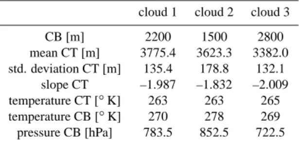
Table 1. Cloudfield parameters.
cloud 1 cloud 2 cloud 3 CB [m] 2200 1500 2800 mean CT [m] 3775.4 3623.3 3382.0 std. deviation CT [m] 135.4 178.8 132.1 slope CT –1.987 –1.832 –2.009 temperature CT [◦K] 263 263 265 temperature CB [◦K] 270 278 269 pressure CB [hPa] 783.5 852.5 722.5
results. In this study a full 3-D radiative transfer calculation is performed using a Monte Carlo algorithm.
To describe the variability of the cloud top no constant value, like –5/3 for the slope of the power spectrum, is imple-mented. Instead high-resolution radar and ceilometer mea-surements are used to derive the variability especially from cloud top. Atmospheric parameters used in this study like wind, temperature, and pressure have been recorded simulta-neously at the Meteorological Observatory Lindenberg.
2 Methodology
2.1 Simulation of cloud fields
In this study measurements of three clouds are chosen to simulate the cloud fields for radiative transfer calculations. All clouds are assumed to consist completely of liquid wa-ter. The first ice particles in super cooled clouds appear at temperatures between 263◦K and 258◦K (Lamb, 2002). The cloud top temperature of all three selected clouds are above 263◦K. In Table 1 the simulated cloud fields are char-acterised (CT = cloud top, CB = cloud base).
The cloud types have been chosen to cover a great part of the natural diversity of geometrical cloud characteristic. Cloud 1 is the type geometrical thick cloud with variable top, cloud 2 geometrical thick with less variable cloud top and cloud 3 represents a geometrical thin cloud with vari-able top. The fourth type a thin cloud with homogeneous top is not considered, because there was no fitting measure-ments of radar and additional data available. For these three measured clouds the following way of simulating cloud fields for radiative transfer calculations is performed. The time to space transformation of cloud top heights, measured by ver-tical pointing radar is based on the so called “frozen turbu-lence assumption”, which assumes no changes of the cloud field during the measurements.
To generate the 2-D cloud top field from 1-D measure-ment data, the iterative amplitude adjusted Fourier transform (IAAFT) algorithm developed by Schreiber and Schmitz (1996, 2000) was applied. This method is based on the ap-plication of Fourier spectra to characterise two point statistics
of spatial or temporal data. Fourier methods have been used widely in previous studies for cloud modelling (e.g. Barker and Davies, 1992). Using the IAAFT algorithm the step from a one-dimensional time series to a two-dimensional data field has been done. The improvement after applying the IAAFT is that the simulated field and the measured time series of cloud top height are equal in power spectrum and the ampli-tude distribution, respectively. From a measured time series, sn(with n is time or space) with N values, the power
spec-trum Sk(with k wave numbers) is calculated as
Sk2= X n sne i2π kn N 2 . (1)
The relevant value describing the variability of the time series is the slope of a power law regression of the power spectrum and the corresponding wave numbers. A straight line con-tinuation of the slope in the scope of higher frequencies is dependent on the absence of scale breaks in the power spec-trum. Furthermore a sorted list of the measured values sn
is necessary for the IAAFT algorithm. The iteration starts with a random shuffle of sn. The first two steps of the
algo-rithm are the adjustment of 1) the Fourier coefficients and 2) the amplitudes. To achieve the desired power spectrum the Fourier transform of the time series is calculated in each it-eration. The absolute values of the coefficients are replaced by those from the measured time series while the phases are retained. A backward transform of these coefficients would produce an amplitude distribution which is not the same as the measured one. Therefore the second step is the adjust-ment of the amplitude distribution, where the amplitudes are sorted and replaced by the sorted values of the original val-ues. These two steps of the iteration have to be repeated until the power spectrum and the amplitude distribution of gener-ated and measured values are matching in sufficient condi-tions.
The derivation of a 2-D variability grid from a 1-D spec-trum with the assumption of isotropic statistics leads to an underestimation of the variance of the 2-D field. This means that the slope of a single row of the 2-D field is much lower then the slope of the 1-D time series. This problem is dis-cussed in Austin et al. (1994), and they propose to use
γ = β − 1 (2)
where β is the slope of the 1-D spectrum of the measured time series and γ is the spectrum that produces a 2-D field consisting of the 1-D value β. In other words, a backward transform of the 2-D Fourier coefficients derived from γ yields in a field where the mean slope of the power spectra of every row and column is around β.
So, cloud top fields were generated consisting of the same power spectrum and amplitude distribution as the 1-D mea-sured time series of cloud top height.
The vertical resolution due to the measurements is as-signed to the 2-D field by the IAAFT. To get a higher vertical
F. Richter et al.: Influence of cloud top variability on radiative transfer 4701
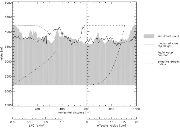
Fig. 1. Measured and simulated cloud top height, subadiabatic LWC profile and adiabatic profile of the effective radius.
resolution of cloud tops for the 3-D cloud field, a linear in-terpolation of the cumulative amplitude distribution is per-formed. So the second step of the IAAFT, the amplitude ad-justment, is done using a refined amplitude distribution.
The vertical dimension of the cloud field is characterised by a subadiabatic liquid water content (LWC) and an adia-batic profile of the effective radius. The LWC profile is based on the study of Chin et al. (2000). In this study a weighting function is applied to describe the subadiabatic character of the profile. This weighting function is given by
f (ˆz) = exp(−α · ˆzβ) (3)
where ˆz is the scaled height within the cloud and α and β are positive constants. In the study Chin et al. (2000) give two types of weighting functions: one is related to subadi-abatic conditions involving cloud top entrainment alone and the other considers both cloud top entrainment and drizzle effects. To ensure the validity of Mie theory for calculation of optical properties the first type was chosen, with the pa-rameterisation of α=1.375 and β=4. The value of α is rec-ommended by Chin et al. (2000) and with β=4 a strong cloud top entrainment is simulated. The weighting function given above weights an adiabatic LWC (LWCad) profile to a
suba-diabatic one (LWCsubad) in the following way
LWCsubad(ˆz)=LWCad(ˆz) · f (ˆz) (4)
The adiabatic LWC profile and the weighting function are calculated from cloud base to the highest cloud top. Then the accordant values for the discretised heights are interpolated and allocated to the overall cloud level.
The adiabatic profile of the effective radius is calculated using the study of Brenguier et al. (2000). The way of calcu-lation is the following,
LWCad(h)=Cw· h, (5) rvad(h)= (A · h) 1 3 · N− 1 3 ad , (6) with: A= Cw 4 3·π·ρw , read(h)= k− 1 3 · rv ad (7) =(A·h)13·(k·Nad)− 1 3 and rsad = k 1 6 · rv ad (8)
Here, Cw is the moist adiabatic condensate coefficient, h is
the altitude above cloud base, ρwthe liquid water density, rv
the mean volume radius, rethe droplet effective radius and rs
the mean surface radius of the droplet size distribution. The parameter k relates rv and re and N is the droplet number
concentration in the cloud. The subscript “ad” for N , re, rv
and rs refers to the adiabatic values. According to Brenguier
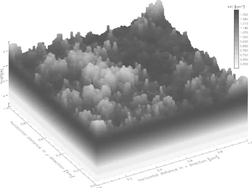
Fig. 2. LWC of the 3-D simulated cloud field.
et al. (2000) k is set to 0.67 for continental air masses and Nadis 250 cm−3representing polluted air.
This combination of a non-adiabatic LWC and an adiabatic profile of the effective radius is corresponding to the term of “inhomogeneous mixing”, mentioned in Baker et al. (1980). This mixing scheme takes place when the time of evaporation of a droplet with radius r is smaller than the time for the com-plete mixing process in the layer. In this case all droplet-radii in the volume affected by entrainment completely evaporate. Figure 1 shows measured time series of cloud top height, a slice of geometrical properties of the simulated cloud field, and profiles of LWC and effective radius. Figure 2 illustrates the three-dimensional cloud field based on these data. As the counterpart to the cloud field with heterogeneous top a field with homogeneous cloud top has been generated using the mean cloud top height of the measured data.
2.2 Monte Carlo simulations
Monte Carlo simulations are performed with the model MC-UNIK, described in Macke et al. (1999). The model assumes periodic boundary conditions in x and y-direction. Each simulation runs with 106 photons, which are uniformly re-leased at the top of the domain. The Monte Carlo model is equipped with the local estimate approch for example de-scribed by Barker et al. (2003). This approach enables to cal-culate reflectances with a smaller amount of injected photons by tracking secondary photons released on every scattering event on there direct way to the detector.
The solar zenith angle is set to 0◦, 30◦and 60◦, the solar azimuth angle is constant at 0◦; observation angles are 0◦, 30◦and 60◦for zenith angle and 0◦, 60◦, 120◦and 180◦for azimuth angle, respectively. Cloud optical properties, like volume extinction coefficent, single scattering albedo, and phase function are calculated by Mie theorie for a wavelength of 0.6 µm assuming a modified gamma distribution for cloud droplet sizes.
Outside the cloudy regions Rayleigh scattering has been applied, inside the cloud Rayleigh and Mie scattering are considered. The absorption of molecules has been neglected. The surface albedo is examined as lambertian reflection. The value is calculated from a bidirectional reflectance dis-tribution function (BRDF) for pasture land. This albedo is also known as “white-sky” albedo (Lucht, 2000). The pa-rameterisation of the BRDF for pasture land is taken from Rahman et al. (1993).
3 Results
An advantage of this study is the use of cloud top variability from radar data. In many studies, power spectra are repre-sented via their slopes in log-log plots calculated by least squares linear regression (assuming power law behaviour). Already Loeb et al. (1998) assumed the widely used slope of –5/3 to generate cloud top fields. The analysis of the mea-sured time series revealed that the slopes with values of−1.8 to−2.0 are always larger than −5/3 (Fig. 3). Thus lower
F. Richter et al.: Influence of cloud top variability on radiative transfer 4703
Fig. 3. Comparison of calculated power spectra.
frequencies and with them the spatially (or temporally) larger variabilities play an important role for the description of the cloud top variance. So in this study the spectra of the mea-sured cloud top data were used to generate cloud top fields.
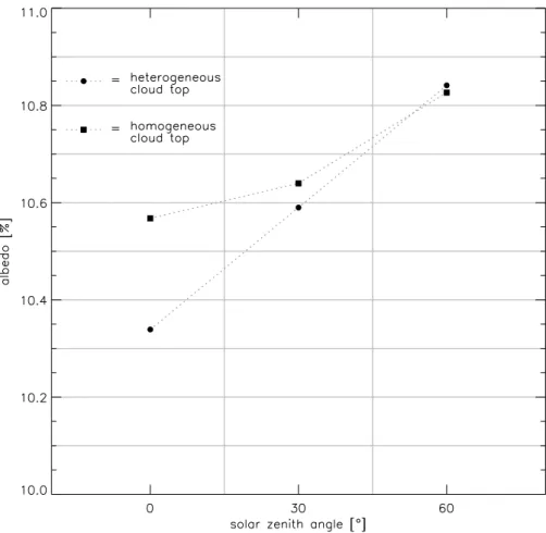
The focus of this study is the comparison of the radia-tive transfer results regarding the differences between clouds with homogeneous and heterogeneous tops. The albedo as the mean value over the whole cloud field provides a first overview. Reflectances in several directions deliver more insight. Figure 4 shows the calculated albedo values for cloud 1 and Table 2 summarises the albedo results for all three clouds. The calculated difference is defined as hetero-geneous albedo minus homohetero-geneous one. Here the albedo for heterogeneous cloud top is lower in most cases and in-creases with increasing solar zenith angle (θsun). The largest
difference is about 1.1%.
Figure 4 indicates that besides cloud top variability also the illumination angle (here only changes in solar zenith an-gles) influences the albedo.
There are higher albedo values with increasing solar zenith angle (θsun), whereas the differences between homogeneous
and heterogeneous cloud top are decreasing. According to the one-dimensional radiative transfer effect (Varnai and Davies, 1999) one reason of the albedo increase with increas-ing θsunis that cloud particles scatter light preferable in
for-ward direction, whereby for overhead sun the solar radiation penetrates deeper into the cloud. This behaviour is well illus-trated by the comparison of the photons’ penetration depth of
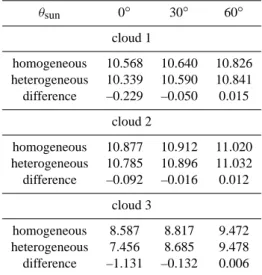
Table 2. Calculated albedo values [%] for the different cloud fields
and solar zenith angle (θsun), the difference is defined as
heteroge-neous minus homogeheteroge-neous albedo value.
θsun 0◦ 30◦ 60◦ cloud 1 homogeneous 10.568 10.640 10.826 heterogeneous 10.339 10.590 10.841 difference –0.229 –0.050 0.015 cloud 2 homogeneous 10.877 10.912 11.020 heterogeneous 10.785 10.896 11.032 difference –0.092 –0.016 0.012 cloud 3 homogeneous 8.587 8.817 9.472 heterogeneous 7.456 8.685 9.478 difference –1.131 –0.132 0.006
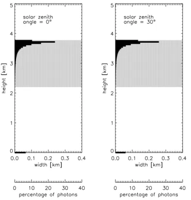
the different illumination angles (Figs. 5, 6 for cloud 1). The penetration depth is used as the measure for the lowest z-position photons reach on their path through the cloud. This position mirrors the optical properties of the so far travelled path.
Fig. 4. Mean albedo values for cloud 1.
Furthermore cloud fields tend to appear more homoge-neous from oblique directions than from above, which en-hances the albedo increase mentioned above (Varnai and Davies, 1999). The cause of the deeper penetration at hetero-geneous cloud tops is the larger surface which leads to more transitions between cloudy parts and non-cloudy ones (Var-nai and Davies, 1999). This added transport into the cloud is also pictured by transmission and absorption (Table 3). The simulated albedo values for cloud 2 and 3 are similar showing increasing albedo values and decreasing differences between homogeneous and heterogeneous tops with increas-ing θsun. The significant difference between homogeneous
and heterogeneous cloud top at θsun=0◦is 0.2% for cloud 1.
Cloud 2 with less variability shows only a difference of 0.1% and the thin and variable cloud 3 shows the largest difference of 1.1%. The high transmission of cloud 3 with simultane-ously low absorption is caused by the short vertical expan-sion of this cloud.
The results mentioned above already denote some aspects of the influence that cloud top variability has on radiative transfer, which is first the lower albedo of heterogeneous cloud top and second the larger penetration depth. Now the effects on reflectances are focussed. Reflectances are
calcu-lated for nine observation angles, for 30◦and 60◦zenith with changes in azimuth of 0◦, 60◦, 120◦, and 180◦, respectively, and the direction of 0◦zenith and 0◦azimuth.
The reflectances of these observation angles are simulated for the three solar zenith angles of 0◦ (Fig. 7), 30◦ and 60◦zenith and 0◦azimuth.
Figure 7 shows the calculated reflectances for cloud 1 as mean values over the cloud field with corresponding mini-mum and maximini-mum values. The azimuth angle of illumi-nation is 0◦, so the azimuth observation angle of 0◦ is the backward direction relative to illumination, 180◦is forward and 60◦and 120◦are sideways, respectively. The reflectance is defined as the ratio of reflected to incident radiation. The variability of the reflectances for homogeneous cloud tops shown in Fig. 7 is the result of the uncertainty of the Monte Carlo model. These uncertainty is determined by the ran-dom nature of the Monte Carlo model and by using the local estimation approach with an obviously too low number of simulated photons.
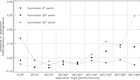
Figures 8 and 9 show the calculated differences, defined as heterogeneous reflectance minus homogeneous one. The maximum difference of the mean reflectances between ho-mogeneous and heterogeneous cloud top is approximately
F. Richter et al.: Influence of cloud top variability on radiative transfer 4705
Fig. 5. Penetration depth of cloud 1 (homogeneous top) for different solar zenith angles.
Fig. 6. Penetration depth of cloud 1 (heterogeneous top) for different solar zenith angles.
Fig. 7. Reflectances of cloud 1 (θsun=0◦) for different observation angles.
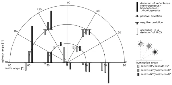
F. Richter et al.: Influence of cloud top variability on radiative transfer 4707
Fig. 9. Deviation of reflectance ((heterogeneous – homogeneous)/homogeneous) for several illumination and observation angles.
0.3, which is 30% of illumination. The largest differences appear in forward and backward direction relative to illu-mination direction, whereas the differences have a negative maximum in backward direction (homogeneous > heteroge-neous) and a positive one in forward direction.
The largest negative difference is found in backward direc-tion when the zenith angles of illuminadirec-tion and observadirec-tion are equal. The maximum positive difference is found in for-ward direction for equal zenith angles of illumination and observation.
The preferred forward direction can be explained by the forward peak of the Mie phase function. The probability that a photon turns around in the backward direction is very low compared to proceeding in forward direction. As mentioned above, the cloud top heterogeneity causes a higher transport into cloudy regions, which leads to more intense scattering. The probability of a complete photon turn is much lower for clouds with heterogeneous tops. Therefore the reflectance in backward direction is lower for clouds with heterogeneous tops then for homogenous ones, which leads to the negative differences shown in the Fig. 8. The largest reflectances ap-pear in forward direction (azimuth angle of 180◦) when the zenith angles of illumination and observation are equal. This behaviour is determined by two effects. One is the domi-nance of the forward peak of Mie scattering, that causes on one hand the escape of the photon in forward direction and on the other hand the deeper penetration for lower solar zenith angles. The deeper penetration causes the distance the pho-ton has to propagate back to the detector to be larger for lower zenith angles than for higher ones. This longer way is the second effect and causes a higher attenuation of the photons’ energy.
Table 3. Transmission and absorption [%] for the different cloud
fields (described in Table 1) and solar zenith angles. variability θsun 0◦ 30◦ 60◦ transmission cloud 1 homogeneous 6.6920 6.1150 4.5183 heterogeneous 8.8190 6.5252 4.2626 cloud 2 homogeneous 3.8751 3.5504 2.6138 heterogeneous 4.5957 3.6744 2.5222 cloud 3 homogeneous 24.9300 22.8276 16.8455 heterogeneous 35.1987 24.0418 16.8273 absorption cloud 1 homogeneous 0.1385 0.1276 0.0963 heterogeneous 0.1705 0.1329 0.0937 cloud 2 homogeneous 0.2619 0.2409 0.1795 heterogeneous 0.3039 0.2471 0.1750 cloud 3 homogeneous 0.0203 0.0192 0.0155 heterogeneous 0.0219 0.0199 0.0162 4 Conclusions
Although earlier studies examined the influence of cloud top variability on radiation, only a few have used measured data with high resolution. Several of the applied techniques have been used in earlier studies, but not necessarily in this way. This study combines them and therefore tries to describe clouds as realistic as possible, always keeping in mind that cloud top variability has to be the only cause of differences in radiative transfer results. The present study should extend
the earlier studies that deal with cloud top heterogeneity ef-fects on radiative transfer in cloudy atmosphere in general.
The Fourier analysis of the measured time series of cloud top height shows that the calculated slopes of the power spec-trum are larger than the widely used assumption of −5/3 owning values of−1.8 to −2.0. So the spatial small-scale variability seems not that important to describe the variance of a cloud top.
The examined cases show an increase of the differences between homogeneous and heterogeneous albedo values at larger cloud top variability. Convective clouds with often larger geometrical cloud top variability are therewith more effected by the influence of these heterogeneity effects than stratiform clouds for example. The solar zenith angle has a larger influence on radiative transfer than cloud top variabil-ity, but for large solar zenith angles the differences of albedo values are negligible.
The differences of reflectances are also larger for higher solar zenith angles, so the neagtive maximum (homogeneous > heterogeneous) appears in backward direction and the positve maximum in forward direction. The largest differ-ence of the mean reflectances between homogeneous and heterogeneous cloud top is approximately 0.3, so it can be important for measurements in these directions. Many atmo-spheric parameters are deviated from satellite measurements. The radiances are gauged at the VIS and IR spectra. The in-fluence of cloud top variability on radiative transfer is not the most important one of course, but might have influence on the accuracy of deviated parameters.
Acknowledgements. The institute of meteorology at the
Technis-che Universit¨at Dresden with C. Bernhofer and all members is gratefully acknowledged for managing the working environment. Special thanks to A. Schwiebus for proof-reading. This paper is based on the master thesis of F. Richter.
Edited by: V. Fomichev
References
Austin, R., England, A., and Wakefield, G.: Special problems in the estimation of power-law spectra as applied to topographical modeling, Geoscience and Remote Sensing, IEEE Transactions on, 32, 928–939, 1994.
Baker, M., Corbin, R. G., and Latham, J.: The influence of entrain-ment on the evolution of cloud droplet spectra: I A model of inhomogeneous mixing, Q. J. Roy. Meteor. Soc., 106, 581–598, 1980.
Barker, H. W. and Davies, J. A.: Solar Radiative Fluxes for Stochas-tic, Scale-invariant Broken Cloud Fields, J. Atmos. Sci., 49, 1115–1126, 1992.
Barker, H. W., Goldstein, R. K., and Stevens, D. E.: Monte Carlo Simulation of Solar Reflectances for Cloudy Atmospheres, J. At-mos. Sci., 60, 1881–1894, 2003.
Brenguier, J.-L., Pawlowska, H., Sch¨uller, L., Preusker, R., Fischer, J., and Fouquart, Y.: Radiative Properties of Boundary Layer Clouds: Droplet Effective Radius versus Number Concentration, J. Atmos. Sci., 57, 803–821, 2000.
Chin, H.-N. S., Rodriguez, D. J., Cederwall, R. T., Chuang, C. C., Grossman, A. S., Yio, J. J., Fu, Q., and Miller, M. A.: A Micro-physical Retrieval Scheme for Continental Low-Level Stratiform Clouds: Impacts of the Subadiabatic Character on Microphysi-cal Properties and Radiation Budgets, Mon. Weather Rev., 128, 2511–2527, 2000.
Lamb, D.: Encyclopedia of atmospheric sciences, Academic Press, 2002.
Loeb, N. G. and Coakley, J. A. J.: Inference of Marine Stratus Cloud Optical Depths from Satellite Measurements: Does 1D Theory Apply?, J. Climate, 11, 215–233, 1998.
Loeb, N. G., Varnai, T., and Winker, D. M.: Influence of Subpixel-Scale Cloud-Top Structure on Reflectances from Overcast Strat-iform Cloud Layers, J. Atmos. Sci., 55, 2960–2973, 1998. Lucht, W.: An algorithm for the retrieval of albedo from space using
semiempirical BRDF models, IEEE Transactions on Geoscience and Remote Sensing, 38, 977–998, 2000.
Macke, A., Mitchell, D., and Bremen, L.: Monte Carlo Radiative Transfer Calculations for Inhomogeneous Mixed Phase Clouds, Physics and Chemistry of the Earth, Part B: Hydrology, Oceans Atmos., 24, 237–241, 1999.
Marshak, A., Davis, A., and Titov, G.: The verisimilitude of the independent pixel approximation used in cloud remote sensing, Remote Sens. Environ., 52, 71–78, 1995a.
Marshak, A., Davis, A., Wiscombe, W., and Cahalan, R.: Radia-tive smoothing in fractal clouds, J. Geophys. Res., 100, 26 247– 26 262, 1995b.
Rahman, H., Verstraete, M. M., and Pinty, B.: Coupled surface-atmosphere reflectance (CSAR) model. 1: Model description and inversion on synthetic data, J. Geophys. Res., 98, 20 779–20 801, 1993.
R¨ais¨anen, P., Barker, W. H., Khairoutdinov Marat, F., Li, J., and Randall, A. D.: Stochastic generation of subgrid-scale cloudy columns for large-scale models, Q. J. Roy. Meteor. Soc., 130, 2047–2067, 2004.
Randall, D., Khairoutdinov, M., Arakawa, A., and Grabowski, W.: Breaking the Cloud Parameterization Deadlock, B. Am. Meteor. Soc., 84, 1547–1564, 2003.
Schreiber, T. and Schmitz, A.: Improved surrogate data for nonlin-earity tests, Phys. Rev. Lett., 77, 635–638, 1996.
Schreiber, T. and Schmitz, A.: Surrogate time series, Physica D, 142, 346–382, 2000.
Varnai, T. and Davies, R.: Effects of Cloud Heterogeneities on Shortwave Radiation: Comparison of Cloud-Top Variability and Internal Heterogeneity, J. Atmos. Sci., 56, 4206–4224, 1999.