Time dependent dispersivity behavior of non-reactive solutes in a system of parallel fractures

(1)

HAL Id: hal-00298703

https://hal.archives-ouvertes.fr/hal-00298703

Submitted on 7 Jun 2006

HAL is a multi-disciplinary open access

archive for the deposit and dissemination of sci-entific research documents, whether they are pub-lished or not. The documents may come from teaching and research institutions in France or abroad, or from public or private research centers.

L’archive ouverte pluridisciplinaire HAL, est destinée au dépôt et à la diffusion de documents scientifiques de niveau recherche, publiés ou non, émanant des établissements d’enseignement et de recherche français ou étrangers, des laboratoires publics ou privés.

Time dependent dispersivity behavior of non-reactive

solutes in a system of parallel fractures

G. Suresh Kumar, M. Sekhar, D. Misra

To cite this version:

G. Suresh Kumar, M. Sekhar, D. Misra. Time dependent dispersivity behavior of non-reactive so-lutes in a system of parallel fractures. Hydrology and Earth System Sciences Discussions, European Geosciences Union, 2006, 3 (3), pp.895-923. �hal-00298703�

(2)

HESSD

3, 895–923, 2006

Dispersivity behavior of non-reactive solutes in fractures

G. Suresh Kumar et al.

Title Page Abstract Introduction Conclusions References Tables Figures J I J I Back Close Full Screen / Esc Printer-friendly Version

Interactive Discussion

EGU

Hydrol. Earth Syst. Sci. Discuss., 3, 895–923, 2006 www.hydrol-earth-syst-sci-discuss.net/3/895/2006/ © Author(s) 2006. This work is licensed

under a Creative Commons License.

Hydrology and Earth System Sciences Discussions

Papers published in Hydrology and Earth System Sciences Discussions are under open-access review for the journal Hydrology and Earth System Sciences

Time dependent dispersivity behavior of

non-reactive solutes in a system of

parallel fractures

G. Suresh Kumar1, M. Sekhar2, and D. Misra3

1

Department of Civil Engineering, Queens University, Kingston, Canada

2

Department of Civil Engineering, Indian Institute of Science, Bangalore, India

3

Department of Mining and Geological Engineering, University of Alaska, Fairbanks, USA Received: 16 March 2006 – Accepted: 24 March 2006 – Published: 7 June 2006

(3)

HESSD

3, 895–923, 2006

EGU

Abstract

In order to obtain meaningful predictions of contaminant transport, an accurate way of quantifying dispersivity needs to be developed. Results from the theoretical studies suggest that dispersion and the associated dispersivity is non-fickian near the source of contaminant and it grows with travel time and distance. In most tests of a limited

5

duration it is quite probable that the asymptotic regime is not reached, and a proper interpretation of the test should be based on the time-dependent results due to the dif-ficulty associated with the expensive experimental setups added to the marked scarcity of field data. An attempt has been made using spatial moment analysis to evaluate the time dependent dispersivity for a system of parallel fractures with matrix diffusion. The

10

study is limited to non-reactive solutes, having a constant continuous source. An em-pirical relation to evaluate the dispersivity was developed by us based on the sensitivity analysis, when distinct parallel fractures have constant aperture width and is found to be functions of matrix porosity, matrix diffusion coefficient and injected fracture veloc-ity at pre-asymptotic stage. The system becomes more complex when the aperture

15

widths of the distinct parallel fractures are varied, as it appears that the initial develop-ment period of non-fickian behavior may be long due to the continuous lateral mixing of the solute body. It is found that dispersivity at pre-asymptotic regime increases with the coefficient of variation for distinct parallel fractures with varying aperture widths.

1 Introduction 20

The movement and mixing of solutes in fractured media is of particular interest in an en-vironmental context because of the possibility of very rapid and extensive movement of contaminants through fractures, cracks, or fissures in otherwise low-permeability rock (Gelhar, 1993). Analysis of flow and solute transport in a single fracture provides a basis for understanding contaminant migration in fractured porous media. Such

knowl-25

(4)

HESSD

3, 895–923, 2006

EGU

assessing the characteristics of a fractured aquitard in ground-water remediation or protection work. Dispersivity is established as one of the key uncertain parameters that influence the concentration at accessible-environment compliance points.

Generally, measurement of transport properties in a complex geologic media be-comes a challenging task. Many experimental investigations of solute transport in

sin-5

gle fractures have been conducted in the laboratory (Sharp, 1970; Iwai, 1976; Grisak et al., 1980; Moreno et al., 1985; Schrauf and Evans, 1985; Abelin, 1986; Raven et al., 1988; Rudolph et al., 1991). These investigations have produced measure-ments of fracture properties and have provided an understanding of the processes controlling solute migration, notably fracture dispersion, matrix diffusion, and

chan-10

neling. Since, matrix diffusion influences the resultant dispersion along the fracture, significantly, at the scale of a single fracture, the measurement of dispersivity result-ing from a fracture-matrix coupled system has become a difficult target. Also since, dispersivity is a measure of the variability in the fluid velocity affecting the advection of dissolved constituents in ground water (Gelhar et al., 1992), and matrix diffusion is

usu-15

ally described as the process by which dissolved constituents diffuse into or out of the primary porosity of the rock-matrix, the resulting spreading of solutes, arising from the simultaneous influences of both longitudinal dispersion (along the fracture), and matrix diffusion (across the fracture) is important to performance assessment and must be captured in the transport models. Only the largest heterogeneities are represented

ex-20

plicitly in the site-scale model; all dispersion caused by smaller-scale features must be represented through the use of a dispersion model. Numerous groundwater transport studies have been conducted at a variety of scales, and the results are compiled using the dispersivity as the correlating parameter. There have been significant studies of heterogeneous field scale media leading to a time-dependent dispersivity (e.g. Gelhar

25

and Axeness, 1983, among others) with the assumption of an infinite domain. The temporal effects imply that the dispersive flux has cumulative effects of previous times, which is typical for a non-Fickian model (Scheidegger, 1960).

(5)

HESSD

3, 895–923, 2006

EGU

not include the coupling effect between fracture and matrix. For example, Horne and Rodriguez (1983) used a method similar to Taylor and Geoffrey (1953) to derive an expression for the net longitudinal dispersivity, for flow in a fracture. It is to be noted that the dispersivity was related as a function of fracture aperture, flow velocity and molecular diffusion, while the influence of the rock matrix was not considered (Gilardi,

5

1984). McKay et al. (1993) had to choose the values of dispersivity for a limited range between 0.2–1.2 m. In general, for single-phase flow, the dispersivity of a fracture is deduced from the statistics of the aperture distribution, using stochastic theory (Keller, 1997). Thus, no attention has been provided to the dispersivity behavior resulting from the coupled effect of fracture and rock matrix.

10

Analytical solutions have been developed for solute transport through an idealized fracture in a homogeneous porous matrix by reducing the transport equation in a two-dimensional domain to two coupled one-two-dimensional problems (Tang et al., 1981; Grisak and Pickens, 1980). Neretnieks et al. (1982) derived a solution assuming negligible dispersion in the fracture. This effect was added in the solution of Tang

15

et al. (1981), which is widely used for model comparison.

The matrix diffusion concept of transport of fractured geologic media has been the basis of numerous mathematical models. The most widely used model involves ad-vective and dispersive transport in the fracture coupled with diffusive transport into the porous matrix (Tang et al., 1981; Maloszewski and Zuber, 1985; Moench, 1995). This

20

model and its successors have been used successfully to fit a number of field tracer tests in fractured rock (e.g., Malozewski and Zuber, 1993; Moench, 1995). In fact these models have achieved such acceptance that it has been suggested that an extended breakthrough tail indicates that matrix diffusion has influenced transport (Tsang, 1995; Meigs et al., 1997). The model of Tang et al. (1981) was later extended to a system of

25

parallel fractures. To mention a few, Grisak and Pickens (1980), Kennedy and Lennox (1995), Jardine et al. (1999), Hara et al. (2000), Becker and Shapiro (2000), Callahan et al. (2000) have used the conceptual model developed by Sudicky and Frind (1982) and Tang et al. (1981) for the purpose of their model development and validation of

(6)

HESSD

3, 895–923, 2006

EGU

their model outcomes.

There are several mechanisms giving dispersion or spreading of a concentration pulse injected into a fractured porous system: (1) molecular diffusion in the fluid, (2) velocity variations in the fluid within individual fracture (microscopic dispersion), (3) ve-locity variations between different fractures (macroscopic dispersion), and (4) chemical

5

and physical interactions with the associated solid matrix (Rasmuson, 1985). In the present paper we concentrate on the dispersivity behavior caused by the macroscopic dispersion and the physical interaction with the solid matrix as it is one of the less understood physical parameters in the modeling of contaminant transport. The study of this parameter has been the subject of considerable research over the past several

10

years (Gelhar, 1993; Woodbury, 1997; Stafford et al., 1998). The difficulty associated with these studies had been the high cost of conducting the required experimental tests and the marked scarcity of the field data (Al-Suwaiyan, 1998). Also, in most experiments of a limited duration it is quite probable that the asymptotic regime is not reached, and a proper interpretation of the test should be based on the time-dependent

15

results (Neretnieks et al., 1982; Moreno et al., 1985; Dagan, 1988).

Moment analysis is a very useful technique used to understand the heterogeneous system of transport in fracture-matrix systems or porous media better. Instead of solv-ing for the actual concentration along the fracture, the original governsolv-ing equations are modified to solve for simplified, but physically important, global quantity referred to as

20

the spatial moments (Goltz and Roberts, 1987; Valocchi, 1989). This global variable can eventually be combined to study the overall impact of different processes on the evolution of pollutant plume (spatial moments). In this paper, we shall investigate the time dependent behavior of effective values of dispersivity by the method of spatial moments and its behavior is studied at pre-asymptotic stage.

(7)

HESSD

3, 895–923, 2006

EGU

2 Physical system and governing equations

The complex network of fractures consisting of both primary and secondary fractures is illustrated in Fig. 1. The primary fractures are assumed to have parallel smooth walls. Two cases are analyzed one with a system of distinct parallel fractures having constant aperture width while the other having different aperture widths. The migration

5

of the dissolved contaminant plumes in a system of distinct parallel fractures is mod-eled by coupled partial differential equations, one describing the transport along the fracture while the other describing the transport into the porous matrix (Sudicky and Frind, 1982). The system of equations for a constant continuous source along with the boundary conditions is as follows.

10

The equation for the fracture is given by

∂c_f ∂t = −vf ∂c_f ∂x + DL ∂2c_f ∂x2 − q b (1)

The equation for the matrix is given by

∂c_m ∂t = Dm ∂2c_m ∂y2 (2) where, q=−θD_m∂cm ∂y and DL=αLv+Dm. 15

Here c_f and c_m are the concentrations of solute in fracture and matrix respectively (M/L3), v_f is the ground water velocity in the fracture (L/T), 2b is the fracture aperture (L), D_Lis the hydrodynamic dispersion coefficient (L2/T), D_m is the molecular diffusion coefficient (L2/T), and q is the diffusive flux (source/sink) perpendicular to the fracture axis (M/L2T−1).

20

The initial and boundary conditions for the fracture and matrix system, respectively, are:

(8)

HESSD

3, 895–923, 2006

Title Page Abstract Introduction Conclusions References Tables Figures J I J I Back Close Full Screen / Esc Printer-friendly Version Interactive Discussion EGU c_m(x, y, 0)= 0; c_m(x, b, t)= c_f(x, t); ∂cm ∂y (x,Lm,t) (4)

where L_f is the length of the fracture and L_mis the half fracture spacing (perpendicular to the fracture axis).

The first spatial moment characterizing the displacement of the center of mass and the second spatial moment characterizing the spread around the center of mass of the

5

solute are obtained from the concentration distribution in fracture using an approach described by Guven et al. (1984). These expressions are valid for concentration pulse sources. Since a constant continuous source is used as a boundary condition at the inlet of the fracture in the present study, a first derivative of the concentration in the fracture is used to obtain an equivalent pulse in order to use these expressions. The

10

study is limited to non-reactive solutes.

By using the governing equations referred in the appendices, which permit determi-nation of spatial moments based on the mean and standard deviation, it is possible to assess how effective parameters behave with respect to the solute transport pa-rameters. In particular, an effective velocity, an effective dispersion coefficient and an

15

effective dispersivity will be computed in terms of model parameters. These effec-tive parameters are local equilibrium model equivalents, which approximately duplicate the concentration responses of the physical non-equilibrium model. The effective pa-rameters are papa-rameters, which would be inferred from applying the local equilibrium transport model to an observed spatial concentration distribution (Goltz and Robertz,

20

1987). Use of these effective parameters will aid in understanding how the general behavior of the spatial concentration distributions differ.

(9)

HESSD

3, 895–923, 2006

EGU

3 Behavior of mobile spatial distributions

3.1 Parallel multiple fractures with constant apertures

Figures 2–7 show how dispersivity behaves as a function of time, in a system of constant discrete multiple-parallel fractures, for local fracture dispersivity, half fracture spacing, fracture velocity, matrix diffusion coefficient and matrix porosity, respectively.

5

The range of solute transport parameters was chosen that ensures the asymptotic region and the data set are provided in Table 1. Laboratory data of Neretniek’s et al. (1982) and Moreno et al. (1985) provide the approximate choice of the system pa-rameters, taken for sensitivity analyses. Figure 2 illustrates the time rate of change of effective dispersivity, for various local fracture dispersivities. In a homogeneous porous

10

system with a conservative solute, the value of dispersivity will be a constant equal to the local dispersivity. But the physically non-equilibrium fracture-matrix system shows an order of increase of dispersivity from the local fracture dispersivity with time, before it reaches a constant asymptotic value. Initially, all the mass is associated with mobile fluids in the fracture region. With time, more and more solute diffuses into the immobile

15

fluids in the porous matrix region, so that eventually, the lateral mixing in the fracture is increased considerably, indicated by the increasing effective dispersivity region at pre-asymptotic stage. It is observed that local fracture dispersivities are insensitive to the choice of the parameters taken. It is observed that the time needed to achieve the asymptotic dispersivity in all cases is nearly the same. It is also noted that the increase

20

in effective dispersivity during the pre-asymptotic regime is not marginal and is nearly two orders of magnitude larger than the local fracture dispersivity considered.

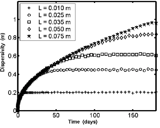
Figure 3 shows the temporal variation of effective dispersivity for various half-fracture spacing. It is interesting to note that all the profiles have similar slopes at pre-asymptotic stage due to the same diffusive transport path into the immobile region

25

from fracture, irrespective of the length of the half fracture spacing considered. The profiles deviate at large times, corresponding to the increase in the half fracture spac-ing. It is important to realize that the simulated profiles take larger time to reach the

(10)

HESSD

3, 895–923, 2006

EGU

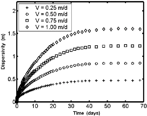
asymptotic region for larger half fracture spacing, as more time is needed to build up the mass from the mobile phase fracture region into the immobile phase matrix region. Figure 4 shows the temporal variation of effective dispersivity for various injected water velocities in the fracture. It is observed that all the profiles have distinct slopes at pre-asymptotic stage because the solute migration distance along the mobile region

5

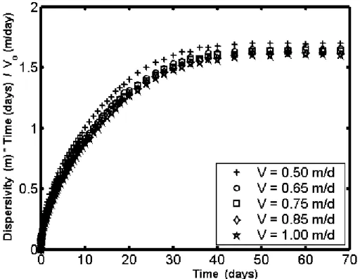
differs considerably with the injected water velocity in the fracture. It is important to realize that the extent of mixing of solutes between fracture and matrix is directly pro-portional to the injected water velocity, as mixing in the fracture is determined by the initial solute mass. Since, it is not possible to predict the residence time of solutes in the fracture, before the start of the experiment, the value of effective dispersivity needs

10

to be evaluated, which is independent of residence time of solutes in the fracture, and in turn, the water velocity. Figure 5 shows the time rate of change of effective dispersiv-ity normalized by the injected water velocdispersiv-ity. This removes the impact of water velocdispersiv-ity. Such analysis assists to evaluate the effective dispersivity given the matrix parameters alone and does not require the value of water velocity and the associated residence

15

time in the fracture.

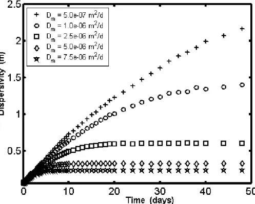
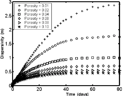
Figures 6 and 7 show the effect of effective matrix diffusion coefficient and matrix porosity on dispersivity. It is to be noted that the slope of the dispersivity profiles are sensitive from the start of the numerical experiment. Matrix porosity and matrix diffusion coefficient have dampening effect on solute spread as they reduce the mass

20

retention time along the fracture. It is to be noted that the time required to reach the asymptoticity is larger under low matrix porosity and matrix diffusion coefficient. A smaller value of such mass transfer coefficients implies a weak coupling between fracture and matrix, and leads to a larger solute mixing.

In order to obtain an empirical relation between the effective dispersivity and other

25

solute transport parameters of the fracture-matrix coupled system, numerical simula-tions are carried out for various sets of parameters and care is taken to ensure that the solutes reach an asymptotic value of dispersivity in all cases. Having obtained the dispersivity profiles, the behavior of effective dispersivity is analyzed during its

(11)

pre-HESSD

3, 895–923, 2006

EGU

asymptotic regime, i.e., before reaching the constant value of dispersivity. Thus, the magnitude of the time dependent effective dispersivity at an early time, before reach-ing a constant value is arrived from these plots and the correspondreach-ing expression is obtained as,

α(t) V_o = t

[θ−0.3×(D−0.143m ×0.037)]× c ₍₅₎ 5

where α(t) is the early time dispersivity, V_ois the injected fracture velocity and c varies from 0.1–0.3. The analysis is extended to compute the time required to attain the asymptotic value and the setting time of the asymptotic dispersivity is given by

t_∞=5 × 10

−6

D_m [c1Lm− c2] (6)

where c₁=−8546θ+5886 and c₂=46. It is observed that the time needed to reach the

10

asymptotic dispersivity depends strongly on the length of the fracture spacing (L_m) and the matrix diffusion coefficient (D_m).

3.2 Parallel multiple fractures with varying apertures

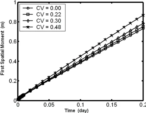
Figure 8 presents the temporal variation of first spatial moment for various coefficients of variation of the fracture aperture described by the ratio of the standard deviation of

15

the fracture aperture to the mean fracture aperture. The system parameters used for these simulations are obtained from Neretniek’s et al. (1982) given in Table 2. It is observed from this plot that the early time behavior of the first spatial moment is linear with time similar to the one observed for a conservative solute in a homogeneous porous medium. It is also observed that increasing the coefficient of variation, results

20

in larger displacements. This is expected as higher coefficient of variation result in decreased loss in mass flux from the fracture into the porous matrix.

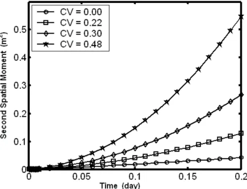
A plot of the temporal evolution of the spatial second moment of the solute is pre-sented in Fig. 9. It is observed that the second spatial moment increases nonlinearly

(12)

HESSD

3, 895–923, 2006

EGU

with time for various coefficients of variation. Before linear behavior is attained, the variance plot is concave, indicating that the macro-dispersion of the solute increases with time. This corresponds to an additional dispersion produced during this period due to solute diffusion into matrix. The linear behavior is attained with lesser displacement along the fracture, when the coefficient of variation is zero.

5

The variation of effective dispersivity with time and solute migration distance are pre-sented in Figs. 10 and 11, respectively. It is observed from the figures that the effective dispersivity has a linear relationship with both space and time at pre-asymptotic stage. It is interesting to note that the effective dispersivity increases as coefficient of variation increases. An attempt has been made to validate the numerical results of the present

10

work with the available data. For this purpose, the numerically simulated dispersivity values have been compared with the laboratory data of Neretnieks et al. (1982) and Moreno et al. (1984). The respective plots are shown in Figs. 11 and 12. It is clear from the plots that the projected model outcomes during the pre-asymptotic dispersiv-ity reasonably match with the laboratory data.

15

4 Conclusion

A numerical model is developed to describe the solute transport in a single fracture with matrix diffusion. The spatial moment analysis of solute front dispersivity in the fracture for transport of non-reactive solutes is presented during pre-asymptotic regime. It is observed that the solute front dispersivity increases with fracture spacing and water

20

velocity, while it decreases with matrix porosity and matrix diffusion coefficient. Results also suggest that the effective dispersivity remains independent of local fracture dis-persivity. The expression for pre-asymptotic dispersivity for the case of non-reactive solutes is also provided. The effect of coefficient of variation of aperture widths of the parallel channels on the solute front dispersivity is analyzed through numerical

mod-25

eling. The results confirm that the higher coefficient of variation, representing a large variation in thicknesses, in a system of parallel fractures, serves to increase the mixing

(13)

HESSD

3, 895–923, 2006

EGU

of solutes. This study thus has demonstrated the applicability of a simple system of parallel fractures with matrix diffusion to estimate the effective dispersivity in a frac-tured, dual porosity media. It is apparent that analyzing mean properties for a system of parallel fractures leads to reasonably good fit with the laboratory data (Figs. 12 and 13).

5

References

Abelin, H.: Migration in a single fracture: An in situ experiment in a natural fracture, Ph.-D. thesis, Dep. Of Chem. Eng., R. Inst. Of Technol., Stockholm, 1986.

AlSuwaiyan, S. M.: Nondeterministic Evaluation of Field Scale-Dispersivity Relation, J. Hydro-logic Engg, 3(3), 215–217, 1998.

10

Becker., M. W. and Shapiro, A. M.: Tracer transport in factured crystallinerock: Evidence of nondiffusive breakthrough tailing, Water Resour. Res., 36(7), 1677–1686, 2000.

Callahan., T. C., Reimus, P. W., Bowman, R. S., and Haga, M. J.: Using multiple experimental methods to determine fracture/matrix interactions and dispersion of nonreactive solutes in saturated volcanic tuff, Water Resour. Res., 36(12), 3547–3585, 2000.

15

Dagan, G.: Time-dependent macrodispersion for solute transport in anisotropic heterogeneous aquifers, Water Resour. Res., 24(9), 1491–1500, 1988.

Gelhar, L. W., Welty, C., and Rehfeldt, K. R.: A critical review of data on field scale dispersion in aquifers, Water Resour. Res., 28(7), 1955–1974, 1992.

Gelhar, L. W. and C. L.: Axness Three-dimensional stochastic analysis of macrodispersion in

20

aquifers, Water Resour. Res., 19(1), 161–180, 1983.

Gelhar, L. W.: Stochastic Subsurface Hydrology, Prentice-Hall, Englewood Cliffs, N. J., 390 pp, 1993.

Gilardi, J. R.: Experimental determination of the effective Taylor dispersivity in a fracture, Dis-sertation of Master of Science, Department of Petroleum Engineering, Stanford University,

25

1984.

Goltz, M. N. and Roberts, P. V.: Using the method of moments to analyse three-dimensional diffusion-limited Solute transport from temporal and spatial perspectives, Water Resour. Res., 23(8), 1575–1585, 1987.

(14)

HESSD

3, 895–923, 2006

EGU Grisak, G. E. and Pickens, J. F.: Solute transport through fractured media, 1, The effect of

matrix diffusion, Water Resour. Res., 16(4), 719–730, 1980.

Grisak, G. E., Pickens, J. F., and Cherry, J. A.: Solute Transport through Fractured Media: 2. Column Study on Fractured Till, Water Resour. Res., 16, 731–739, 1980.

Guven, O., Molz, F. J., and Melville, J. G.: An Analysis of Dispersion in a Stratified Aquifer,

5

Water Resour. Res, 20(10), 1337–1354, 1984.

Hara., S. K. O., Parker, B. L., Jorgensen, P. R., and Cherry, J. A.: Trichloroethane DNAPL flow and mass distribution in naturally fractured clay: Evidence of aperture variability, Water Resour. Res., 36(1), 135–147, 2000.

Horne, R. N. and Rodriguez, F.: Dispersion in Tracer Flow in Fractured Geothermal Systems,

10

Geophys. Res. Lett., 10(4), 289–292, 1983.

Iwai, K.: Fundamental studies of fluid flow through a single fracture, Ph.D. dissertation, Univ. of Calif., Berkeley, 1976.

Jardine., P. M., Sanford, W. E., Gwo, J. P., Reedy, O. C., Hicks, D. S., Riggs, J. S., and Bailey, W. B.: Quantifying diffusive mass transfer in fractured shale bedrock, Water Resour. Res.,

15

35(7), 2015–2030, 1999.

Keller, A. A.: High resolution CAT imaging of fractures in consolidated materials, Int. J. Rock. Mech. Min. Sci., 34(3/4), 358–375, 1997.

Kennedy, C. A. and Lennox, W. C.: Control volume model of solute transport in a single fracture, Water Resour. Res., 31(2), 313–322, 1995.

20

Maloszewski, P. and Zuber, A.: On the theory of tracer experiments in fissured rocks with a porous matrix, J. Hydrol., 79, 333–358, 1985.

Maloszewski, P. and Zuber, A.: Tracer experiments in fissured rocks: matrix diffusion and the validity of models, Water Resour. Res., 29(8), 2723–2735, 1993.

McKay, L. D., Gillham, R. W., and Cherry, J. A.: Field experiments in a fractured clay till 2.

25

Solute and colloid transport, Water Resour. Res., 29(12), 3879–3890, 1993.

Meigs, L. C., Beauheim, R. L., McCord, J. T., Tsang, Y. W., Haggerty, R.: Design, modelling, and current interpretations of the H-19 and H-11 tracer tests at the WIPP site, in: OECD Proceedings – Disposal of radioactive waste, Field tracer experiments: Role in the prediction of radionuclide migration, Synthesis and proceedings of an NEA/EC GEOTRAP Workshop,

30

Cologne, Germany, 28–30 August 1996, OECD/NEA, Paris, France, 1997.

Moench, A. F.: Convergent radial dispersion in a double-porosity aquifer with fracture skin: analytical solution and application to a field experiment in fractured chalk, Water Resour.

(15)

HESSD

3, 895–923, 2006

EGU Res., 31(8), 1823–1835, 1995.

Moreno, L., Neretnieks, I., and Eriksen, T.: Analysis of some laboratory tracer runs in natural fissures, Water Resour. Res., 21(7), 951–958, 1985.

Neretnieks, I., Eriksen, T., and Tahtinen, P.: Tracer Movement in a Single Fissure in Granitic Rock: Some Experimental Results and Their Interpretation, Water Resour. Res., 18(4), 849–

5

858, 1982.

Rasmuson, A.: Analysis of Hydrodynamic Dispersion in Discrete Fracture Networks Using the Method of Moments, Water Resour. Res., 21(11), 1677–1683, 1985.

Raven, K. G., Novakowski, K. S., and Lapcevic, P. A.: Interpretation of field tracer tests of a single fracture using a transient solute storage model, Water Resour. Res., 24(12), 2019–

10

2032, 1988.

Rudolph, D. L., Cherry, J. A., and Farvolden, R. N.: Groundwater flow and solute transport in fractured lacustrine clay near Mexico city, Water Resour. Res., 27(9), 2187–2201, 1991. Scheidegger, A. E.: The physics of flow through porous media, The Macmillan Company, New

York, 1960.

15

Schrauf, T. W. and Evans, D. D.: Laboratory studies of gas flow through a single natural fracture, Water Resour. Res., 22(7), 1038–1050, 1986.

Sharp, J. C.: Fluid flow through fissured media, Ph.-D. dissertation, Imp. College, London, 1970.

Sudicky, E. A. and Frind, E. O.: Contaminant Transport in Fractured Porous Media: Analytical

20

Solutions for a System of Parallel Fractures, Water Resour. Res., 18(6), 1634–1642, 1982. Stafford, P., Toran, L., and McKey, L.: Influence of fracture truncation on dispersion: A dual

permeability model, J. Cont. Hydrol., 30, 79–100, 1998.

Tsang, Y. W.: Study of alternative tracer tests in characterizing transport in fractured rocks, Geophys. Res. Lett., 22(11), 1421–1424, 1995.

25

Tang, D. H., Frind, E. O., and Sudicky, E. A.: Contaminant transport in fractured porous media: Analytical solution for a single fracture, Water Resour. Res., 17(3), 467–480, 1981.

Taylor, Sir G. F. R. S.: Dispersion of Soluble Matter Flowing Slowly Through a Tube, Proc. Roy. Soc. , A 219, 186–203, 1953.

Valocchi, A.: Spatial moment analysis of the transport of kinetically absorbing solutes through

30

stratified aquifers, Water Resour. Res., 25(2), 273–279, 1989.

Woodbury, A. D.: A probabilistic fracture transport model: Application to contaminant transport in a fractured clay deposit, Canadian Geotechnical Journal, 34, 784–798, 1997.

(16)

HESSD

3, 895–923, 2006

EGU

Table 1. Test parameters for Fig. 2.

Figure 2b 2L Vf αL θm Dm (µm) (m) (m/d) _(m) (m2/d) 2 100 0.02 1.0 0.025–0.1 0.1 5×10−7 3 100 0.01–0.075 0.5 0.05 0.1 5×10−6 4 100 0.02 0.5–1.0 0.1 0.1 1.×10−6 5 100 0.02 0.5–1.0 0.1 0.1 1×10−6 6 100 0.02 0.5 0.05 0.05 5×10−7–7.5×10−6 7 100 0.05 0.5 0.05 0.01–0.1 5×10−6

(17)

HESSD

3, 895–923, 2006

EGU

Table 2. The parameters obtained from the data of Neretniek et al. (1982) and Moreno et

al. (1985) for Figs. 11–13.

Index Data of Neretniek et al. (1982) Data of Moreno et al. (1985) Mean Aperture (2b) 0.182 mm 0.14 and 0.15 mm

Mean Dispersivity (αo) 0.027 mm 0.005 and 0.011 mm

Mean Velocity (Vo) 3.65 m/day 5.0 m/day

Diffusion Coefficient (Dm) 8.64e–07 m

2

/day 8.64e–08 m2/day Matrix Porosity (θm) 0.01 0.01

(18)

HESSD

3, 895–923, 2006

EGU

Figure 1. A fracture-matrix system. (a) Conceptualization of a system of smooth parallel multiple fractures having constant aperture widths.

(b) Conceptualization of a system of smooth parallel multiple fractures having variable aperture widths. (c) A single fracture-matrix with the

boundary conditions posed for the solute transport model.

Fig. 1. A fracture-matrix system. (a) Conceptualization of a system of smooth parallel multiple

fractures having constant aperture widths.(b) Conceptualization of a system of smooth parallel

multiple fractures having variable aperture widths.(c) A single fracture-matrix with the boundary

(19)

HESSD

3, 895–923, 2006

EGU

Figure 2. Temporal variation of dispersivity with 2b = 100 μm; 2L = 0.02 m; Vf =

1.0 m/d; θm = 0.1; Dm = 5.0e-07 m2/d

Fig. 2. Temporal variation of dispersivity with 2b=100 µm; 2L=0.02 m; Vf=1.0 m/d; θm=0.1;

Dm=5.0e−07 m

2

(20)

HESSD

3, 895–923, 2006

EGU

Figure 3. Temporal variation of dispersivity with 2b = 100 μm; Vf = 0.5 m/d; αL = 0.05 m; θm = 0.1; Dm = 5.0e-06 m2/d

Fig. 3. Temporal variation of dispersivity with 2b=100 µm; Vf=0.5 m/d; αL=0.05 m; θm=0.1;

Dm=5.0e−06 m

2

(21)

HESSD

3, 895–923, 2006

EGU

Figure 4. Temporal variation of dispersivity with 2b = 100 μm; 2L = 0.02m; αL = 0.05 m; θm = 0.1; Dm = 1.0e-06 m2/d

Fig. 4. Temporal variation of dispersivity with 2b=100 µm; 2L=0.02 m; αL=0.05 m; θm=0.1;

Dm=1.0e−06 m

2

/d.

(22)

HESSD

3, 895–923, 2006

EGU

Figure 5. Temporal variation of dispersivity with 2b = 100 μm; 2L = 0.02m; αL = 0.05 m; θm = 0.1; Dm = 1.0e-06 m2/d

Fig. 5. Temporal variation of dispersivity with 2b=100 µm; 2L=0.02 m; αL=0.05 m; θm=0.1;

Dm=1.0e−06 m

2

(23)

HESSD

3, 895–923, 2006

EGU

Figure 6. Temporal variation of dispersivity with 2b = 100 μm; 2L = 0.02m; Vf = 0.5m; αL = 0.05 m; θm = 0.05

Fig. 6. Temporal variation of dispersivity with 2b=100 µm; 2L=0.02 m; Vf=0.5 m; αL=0.05 m;

(24)

HESSD

3, 895–923, 2006

EGU

Figure 7. Temporal variation of dispersivity with 2b = 100 μm; 2L = 0.05m; Vf = 0.5m; αL = 0.05 m; Dm = 5.0e-06 m2/d

Fig. 7. Temporal variation of dispersivity with 2b=100 µm; 2L=0.05 m; Vf=0.5 m; αL=0.05 m;

Dm=5.0e−06 m

2

/d.

(25)

HESSD

3, 895–923, 2006

EGU

Figure 8. Temporal variation of first spatial moment for various coefficient of variation for the data set presented in Table 2.

Fig. 8. Temporal variation of first spatial moment for various coefficient of variation for the data

set presented in Table 2.

(26)

HESSD

3, 895–923, 2006

EGU

Figure 9. Temporal variation of second spatial moment for various coefficient of variation for the data set presented in Table 2.

Fig. 9. Temporal variation of second spatial moment for various coefficient of variation for the

data set presented in Table 2.

(27)

HESSD

3, 895–923, 2006

EGU

Figure 10. Temporal variation of effective dispersivity for various coefficient of variation for the data set presented in Table 2.

Fig. 10. Temporal variation of effective dispersivity for various coefficient of variation for the

data set presented in Table 2.

(28)

HESSD

3, 895–923, 2006

EGU

Figure 11. A comparison of effective dispersivity simulated by the present model and Neretniek et al. (1982) data.

Fig. 11. A comparison of effective dispersivity simulated by the present model and Neretniek

et al. (1982) data.

(29)

HESSD

3, 895–923, 2006

EGU

Figure 12. A comparison of effective dispersivity simulated by the present model and Neretniek et al. (1982) data: A larger Scale.

Fig. 12. A comparison of effective dispersivity simulated by the present model and Neretniek

(30)

HESSD

3, 895–923, 2006

EGU

Figure 13. A comparison of effective dispersivity simulated by the present model and Moreno et al. (1985) data.

Fig. 13. A comparison of effective dispersivity simulated by the present model and Moreno et