HAL Id: hal-00296935
https://hal.archives-ouvertes.fr/hal-00296935
Submitted on 15 Jun 2006
HAL is a multi-disciplinary open access
archive for the deposit and dissemination of
sci-entific research documents, whether they are
pub-lished or not. The documents may come from
teaching and research institutions in France or
abroad, or from public or private research centers.
L’archive ouverte pluridisciplinaire HAL, est
destinée au dépôt et à la diffusion de documents
scientifiques de niveau recherche, publiés ou non,
émanant des établissements d’enseignement et de
recherche français ou étrangers, des laboratoires
publics ou privés.
EnKF assimilation of simulated spaceborne Doppler
observations of vertical velocity: impact on the
simulation of a supercell thunderstorm and implications
for model-based retrievals
W. E. Lewis, G. J. Tripoli
To cite this version:
W. E. Lewis, G. J. Tripoli. EnKF assimilation of simulated spaceborne Doppler observations of
vertical velocity: impact on the simulation of a supercell thunderstorm and implications for
model-based retrievals. Advances in Geosciences, European Geosciences Union, 2006, 7, pp.343-348.
�hal-00296935�
SRef-ID: 1680-7359/adgeo/2006-7-343 European Geosciences Union
© 2006 Author(s). This work is licensed under a Creative Commons License.
Advances in
Geosciences
EnKF assimilation of simulated spaceborne Doppler observations
of vertical velocity: impact on the simulation of a supercell
thunderstorm and implications for model-based retrievals
W. E. Lewis and G. J. TripoliDepartment of Atmospheric and Oceanic Sciences, University of Wisconsin, Madison, Wisconsin, USA
Received: 31 October 2005 – Revised: 3 December 2005 – Accepted: 6 December 2005 – Published: 15 June 2006
Abstract. Recently, a number of investigations have been
made that point to the robust effectiveness of the Ensem-ble Kalman Filter (EnKF) in convective-scale data assimi-lation. These studies have focused on the assimilation of ground-based Doppler radar observations (i.e. radial veloc-ity and reflectivveloc-ity). The present study differs from these in-vestigations in two important ways. First, in anticipation of future satellite technology, the impact of assimilating space-borne Doppler-retrieved vertical velocity is examined; sec-ond, the potential for the EnKF to provide an alternative to instrument-based microphysical retrievals is investigated.
It is shown that the RMS errors of the analyzed fields pro-duced by assimilation of vertical velocity alone are in gen-eral better than those obtained in previous studies: in most cases assimilation of vertical velocity alone leads to analyses with small errors (e.g. <1 ms−1for velocity components) af-ter only 3 or 4 assimilation cycles. The microphysical fields are notable exceptions, exhibiting lower errors when obser-vations of reflectivity are assimilated together with observa-tions of vertical velocity, likely a result of the closer relation-ship between reflectivity and the microphysical fields them-selves. It is also shown that the spatial distribution of the error estimates improves (i.e. approaches the true errors) as more assimilation cycles are carried out, which could be a significant advantage of EnKF model-based retrievals.
1 Introduction
The Kalman filter (Kalman, 1960) has a rich history of suc-cess in a wide range of applications, but not until a compu-tationally feasible Monte Carlo implementation was devel-oped (Evensen, 1994) did its application to geophysical data assimilation become attractive. The Ensemble Kalman Filter (EnKF), so called because it relies on an ensemble of model forecasts to provide the requisite error statistics, has been ap-Correspondence to: W. E. Lewis
plied to atmospheric data assimilation at scales ranging from the global (Houtekamer and Mitchell, 1998, hereafter HM) to the convective (Snyder and Zhang, 2003, hereafter SZ).
Future generations of satellites are anticipated to include Doppler capability1, thus providing the possibility of hereto-fore unavailable observations of vertical velocity. Convec-tive systems are by definition regions of enhanced vertical motion, and so an EnKF Observing System Simulation Ex-periment (OSSE) conducted on an idealized supercell thun-derstorm, as in SZ, will provide an excellent opportunity for evaluating the potential impact of these data.
Dowell et al. (2004) broached the possibility of employing the EnKF in convective-scale wind and temperature retrieval, and here we extend their results to examine the potential of the EnKF in microphysical retrieval. In addition to forming a posterior estimate that comprises more information than the instrument-based retrieval alone, the EnKF would pro-vide the ability to retrieve model fields which are not directly observable (such as rainfall), as well as provide superior spa-tiotemporal resolution and a straightforward means of quan-tifying retrieval error.
Section 1 sets out a brief review of the Ensemble Kalman Filter. Section 2 provides an overview of the experiment de-sign and methodology. Section 3 presents the results of the experiments, and conclusions are presented in Sect. 4.
2 The Ensemble Kalman Filter
As mentioned above, the EnKF is a Monte Carlo imple-mentation of the optimal linear filter developed by Kalman in 1960. Its implementation is illustrated by the follow-ing: letting xf denote a column vector containing the model
1Im, E. and Durden, S. L.: Spaceborne Atmospheric Radar Technology, Proceedings of the 2005 Earth-Sun System Technol-ogy Conference, http://www.esto.nasa.gov/conferences/estc2005/ author.html, 2005
344 W. E. Lewis and G. J. Tripoli: EnKF assimilation of simulated spaceborne Doppler observations forecast, the analysis xaobtained by assimilating a column
vector, y, of observations is
xa=xf +K(y − H (xf)). (1) H is a measurement operator, possibly nonlinear, which re-lates the model variables to the observations y, and the ma-trix K is known as the Kalman gain. K provides the means for converting the discrepancy between model and observa-tion at a particular point into a smooth increment applied to rest of the model domain. It is defined as
K = PHT(HPHT +R)−1, (2) where P is the error covariance matrix of the model fore-cast xf and R is the observation error covariance matrix. The matrix P has as many elements as the model state size squared (i.e. 1012 or 1014 elements, given a typical NWP model) and is thus impractical to compute directly. In ad-dition, H will not in general be transposable if it is nonlinear. Fortunately these difficulties may be overcome if the covari-ances are computed from an ensemble of model forecasts as demonstrated by HM: PHT = 1 m −1 Xm i=1(x f i − ¯x f i)(H (x f i ) − H (x f i )) T (3) HPHT = 1 m −1 Xm i=1(H (x f i) − H (x f i))(H (x f i) − H (x f i)) T, (4) where the index i varies over the m ensemble members and the H indicates that the measurement operator may indeed be a nonlinear model operator.
Implementation of the EnKF thus requires that an initial ensemble of model states be defined, usually by perturbing a best-guess estimate of the initial state. Then, each ensem-ble member is integrated forward until observations become available, at which point Eqs. (3) and (4) are used to calculate the products PHT and HPHT. The Kalman gain K is then calculated from Eq. (2), and the analysis for each ensemble member may then be computed from Eq. (1). The result is an ensemble of m analyses which are then integrated forward to the next observation time. Since K is computed from an en-semble of model states (rather than propagated according to a linear model, as in the original Kalman filter), it is allowed to evolve in accord with the nonlinear dynamics of the NWP model. This “flow-dependence” is a very attractive feature of the EnKF, and will be addressed further in Sect. 3.
It is important to note that the EnKF (as well as the Kalman filter before it) is an algorithm for propagating the state prob-ability density function (PDF) forward in time, assuming that the PDF is Gaussian and thus requiring only two moments – the mean and covariance – to completely specify it. In this framework, one can think of the m state vectors as random vectors drawn from the PDF, and the mean of these vectors as the best linear estimate (in the minimum variance sense) of the true PDF mean. The covariance matrix P is a measure of the spread of the ensemble members and thus a gauge for
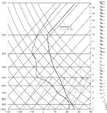
Fig. 1. Environmental sounding used to initialize the simulations. Temperature (◦C) is denoted by the solid line and dewpoint (◦C) by the dashed line. Wind vector magnitude is indicated by half barbs (2.5 m s−1), full barbs (5 m s−1)and flags (25 m s−1)(after Snyder and Zhang, 2003).
the quality of the estimate. The potential usefulness of the information contained in P will be discussed again in sec-tion 3. The extent to which P reflects the true error in the estimate depends in large part on the filter’s optimality, and this in turn depends on a number of factors, among the most important of which is the well-recognized tendency of finite-sized ensembles to underestimate the forecast error covari-ance (Whittaker and Hamill, 2001, hereafter WH).
3 Experiments
The experimental setup is largely the same as that employed in SZ and begins with the environmental sounding shown in Fig. 1. The University of Wisconsin Nonhydrostatic Model-ing System (UW-NMS) (Tripoli, 1992) is initialized with this sounding on a domain employing 35 grid points in each spa-tial dimension. Grid spacing is 2 km in the horizontal, 500 m in the vertical and a time step of 10 s is used in integrating the model forward. Convection is initiated with a warm bub-ble at the surface center of the domain (nx=18, ny=18, nz=1) and 7 ms−1is subtracted from the zonal wind component, u, in order to keep the storm within the computational domain.
In accordance with the above, a 100-minute “Truth” simu-lation (TR) is used to produce simulated observations of both vertical velocity, w, and equivalent reflectivity factor, Ze
(Smith, 1975). Since the minimum detectable signal (MDS) of the spaceborne Doppler instrument is anticipated to be ∼5 dBZ, observations of w and Ze are saved only at those
Table 1. Description of Experiments.
Experiment Field Assimilated Observation Density Observation Frequency
TR (TRUTH) n/a n/a n/a
W2 w 2 km (5 min)−1 Z2 Z 2 km (5 min)−1 WZ2 w, Z 2 km (5 min)−1 5 10 15 20 5 10 15 20 Y (km) −10 −5 0 5 10 15 20 25 5 10 15 20 5 10 15 20 −10 −5 0 5 10 15 20 25 5 10 15 20 5 10 15 20 −10 −5 0 5 10 15 20 25 5 10 15 20 5 10 15 20 X (km) −10 −5 0 5 10 15 20 25 (a) (b) (c) (d)
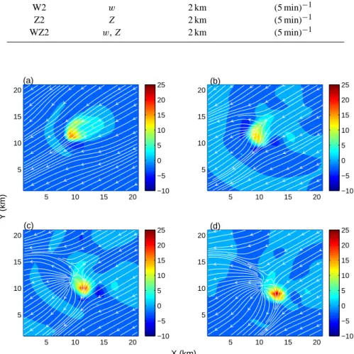
Fig. 2. Vertical velocity, w, at z=6 km (shaded) and surface streamlines at (a) t=30 min, (b) t=45 min, (c) t=60 min, and (d) t=75 min for the “Truth” simulation.
grid points where Zeis greater than or equal to this threshold
value.
Three assimilation experiments are conducted in which the observations as obtained above are assimilated using the EnKF. In the first experiment, denoted W2, observations of w are assimilated every five minutes beginning at t=25 min into the simulation (the point at which the number of observations exceeds several dozen) and is continued until t=100 min. Similarly, experiment Z2 involves the assimilation of Ze, and
experiment WZ2 involves the simulation of both w and Ze.
The experiments are summarized in Table 1.
Each of the assimilation experiments is begun by adding 40 separate realizations of uncorrelated, zero-mean Gaussian random noise to each gridpoint of the environmental sound-ing after it has been interpolated into model space and be-fore the warm bubble is activated, thereby producing a 40-member ensemble. The standard deviation of the noise is 1 ms−1for the wind components and 1 K for the ice-liquid potential temperature, θil. The observation error covariance
matrix, R, is assumed to be diagonal (i.e. observation errors are uncorrelated) and standard errors of 1 ms−1are assumed for the vertical velocity component, w, and a standard error of 5 dBZ is assumed for reflectivity.
Several additional details concerning the precise formula-tion of the EnKF algorithm need to be menformula-tioned. First, a compact covariance localization scheme with local support (Gaspari and Cohn, 1999) is used to reduce the influence of distant, noisy covariance estimates owing to the finite-sized ensemble; in this case, only those elements of the covariance field lying within 6 km of the observation point are allowed to influence the analysis. This choice of localization radius is supported by consideration of the correlation and cross-correlation structure of the model fields as calculated from the ensemble (not shown). In a further effort to improve the optimality of the filter, both a square-root analysis scheme and a covariance inflation scheme as described in WH are employed. An inflation factor of 7% seems to produce the best results in conjunction with the chosen localization radius
346 W. E. Lewis and G. J. Tripoli: EnKF assimilation of simulated spaceborne Doppler observations 20 40 60 80 100 0 1 2 3 4 u (m/s) 20 40 60 80 100 0 1 2 3 4 v (m/s) 20 40 60 80 100 0 1 2 3 4 5 w (m/s) 20 40 60 80 100 0 1 2 3 4 θil (K) 20 40 60 80 100 0 0.5 1 qr (g/kg) 20 40 60 80 100 0 0.05 0.1 0.15 qs (g/kg) (a) (b) (c) (d) (e) (f) TIME (min) RMS ERROR
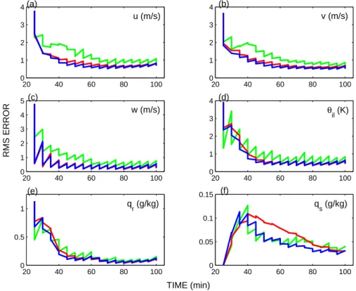
Fig. 3. RMS errors averaged over the domain where Zeexceeds 5 dbz for (a) u, (b) v, (c) w, (d) θil, (e) qr, and (f) qs. Errors for u, v and w
are in units of m s−1. Errors for θil are in K. Errors for qr and qs are in g kg−1. Red line indicates experiment W2, green line indicates Z2,
and blue line indicates WZ2.
of 6 km. Finally, since R is assumed diagonal, observations are assimilated one at a time, allowing the analysis field re-sulting from the assimilation of one observation to become the forecast field for the next, and so on until all observations for a particular time period are assimilated (Anderson and Moore, 1979).
4 Results
The evolution of the “Truth” simulation can be seen in Fig. 2, which depicts vertical velocity (shaded) at z=6 km as well as streamlines of the horizontal wind at the lowest model level over the innermost 20 km of the model domain. At t=30 min (Fig. 2a) the storm has begun to split into right and left-moving cells, as two vertical velocity maxima are evident. By t=45 min (Fig. 2b) the right-moving cell has become dom-inant, as one would expect from the veering wind profile of the environmental sounding. The right-moving cell contin-ues to intensify at t=60 min (Fig. 2c) and t=75 min (Fig. 2d), and an increasingly diffluent pattern is noted in the surface streamlines, indicative of the establishment of a well-defined rear-flanking downdraft.
In order to gauge the improvement of the analysis over time, the RMS errors of the ensemble mean of six model fields – u, v, w, θil, qr , and qs – are calculated. The errors
are averaged over each gridpoint in the model domain where reflectivity equals or exceeds 5 dBZ and thus give a good
in-dicator of filter performance. The errors at gridoints where Ze<5 dBZ are very small, and, since they constitute a
major-ity of the computational domain, their inclusion would serve to mask the robust reduction of error in the area of interest. Figures 3a, b, and c show the evolution of the RMS errors associated with the u, v, and w compnents of the wind, re-spectively, with experiment W2 depicted by the red line, ex-periment Z2 by the green line, and exex-periment WZ2 by the blue line.
Several trends are apparent. First, the largest impact oc-curs during the first few assimilation cycles. Second, the as-similation of reflectivity generally produces inferior results compared to the assimlation of vertical velocity, especially during the first 30 or 40 min of the assimilation. Tong and Xue (2005) noted similar behavior and attributed it to the evolution of the cross covariances associated with reflectiv-ity. Since precipitation begins forming in the simulation only at t=20 min, and frozen precipitation only at t=30 min, it is reasoned that it takes some time for cross covariances be-tween reflectivity and the other model fields to develop and become representative of the actual dynamics. Also of note is the magnitude of the errors. At t=40 min, the errors for u and v have been reduced to ∼1 ms−1 and the errors for wto ∼ 0.5 ms−1. RMS errors this low are not achieved at any point during the 100 min simulation carried out by SZ. This improvement is attributed to the intrinsic value of ver-tical velocity as an observed field relative to observations
10 20 30 5 10 15 20 25 30 35 0.1 0.2 0.3 0.4 0.5 0.6 0.7 0.8 10 20 30 5 10 15 20 25 30 35 0.1 0.2 0.3 0.4 0.5 0.6 0.7 0.8 10 20 30 5 10 15 20 25 30 35 0.01 0.02 0.03 0.04 0.05 0.06 10 20 30 5 10 15 20 25 30 35 0.01 0.02 0.03 0.04 0.05 0.06 (a) q
r true error, t = 30 min (b) qr EnKF predicted error, t = 30 min
(c) q
r true error, t = 70 min (d) qr EnKF predicted error, t = 70 min
X (km)
Y (km)
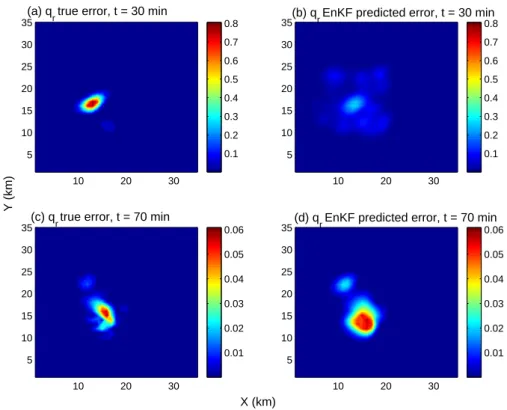
Fig. 4. Comparison of true and predicted errors in g kg−1for qr at the lowest model level. True errors at t=30 min and t=75 min are shown
in (a) and (c) respectively, and predicted errors for t=30 min and t=75 min are shown in (b) and (d) respectively. Note the change in contour level between the two times.
of the horizontal wind, especially in cloud-resolving simu-lations such as the ones here. Not only do vertical velocity observations indicate the location of important features such as up- and downdrafts, they also provide immediate insight into the divergent part of the horizontal wind. Conversely, moving from observations of horizontal wind components to knowledge of the vertical motion field is much trickier (e.g. O’Brien, 1970).
The RMS errors for the ice-liquid potential temperature, θil, are shown in Fig. 3d, and the errors associated with the
rainwater mixing ratio, qr, and snow mixing ratio, qs, are
shown in Figs. 3e and f, respectively. The filter is less ef-ficient in reducing the errors for these fields, with rainwater and especially snow revealing particularly refractory behav-ior. With regard to θil, the reason for the lag in error
reduc-tion vis-a-vis the velocity components is a somewhat more indirect dynamical coupling to the observations. For exam-ple, assimilation of w produces a rapid response in the ana-lyzed w field, and a correspondingly rapid response (though smaller in magnitude) to the u and v fields since the horizon-tal and veritcal motion fields are related via continuity. The coupling of w to the θil field is more complex and involves
diabatic processes, thus requiring a bit more time for the im-pact of the observations to translate to the analysis.
The microphysical fields reveal an interesting reversal of the relative impact of w and Ze, namely that Ze is as
ef-fective (rain) or superior (snow) to w in reducing the RMS errors. Here again, the reasoning is that reflectivity is more
directly linked to the microphysical fields than is vertical ve-locity. Therefore, even though the cross-covariances associ-ated with reflectivity are slow to develop with regard to the dynamical and thermodynamical fields, they develop some-what more quickly with regard to the microphysical fields. It is interesting to note that over time, w becomes as effective as Ze in reducing the microphysical errors, suggesting that
once developed, the cross covariances associated with verti-cal velocity are more robust.
Finally, the potential role of the EnKF in performing model-based retrievals is explored. Given that bulk reduc-tion of RMS error has been demonstrated here as well as in numerous other studies, the ability of the EnKF to pro-duce spatial estimates of retrieval error provides a necessary complement. Shown in Fig. 4 are actual as well as predicted RMS errors for rainwater mixing ratio at the lowest model level. Figures 4a and b refer to true and predicted errors, respectively, at t=30 min, and Figs. 4c and d to true and pre-dicted errors at t=75 min. At t=30 min, the prepre-dicted error field bears little resemblance to the actual error field, other than the identification of the locus of maximum error near x=12 km and y=17 km. Considerable improvement is noted by t=75 min. Indeed, the bimodel spatial distribution of the true error is captured nicely by the EnKF, although the mag-nitude of the error is overestimated by several hundredths of 1 g kg−1, likely as a result of the simplistic covariance infla-tion scheme employed. Further improvement could likely be gained by using a more sophisticated (i.e. adpative) inflation
348 W. E. Lewis and G. J. Tripoli: EnKF assimilation of simulated spaceborne Doppler observations scheme and by increasing the size of the ensemble, but
over-all these results suggest that given a properly tuned filter, a reasonably accurate retrieval of the rain field can be achived after 50 min of assimilation. Similar results hold for the other dynamical, thermodynamical and microphysical fields (not shown).
5 Conclusions
It is shown that assimilation of vertical velocity with an EnKF produces RMS errors which are in general lower than those produced when only ground-based radial velocity is as-similated as in SZ. This result is anticipated given that con-vective systems, such as the supercell thunderstorm under consideration here, are characterized by their enhanced verti-cal motion fields. Accurate placement of up- and downdraft cores is crucial, as is properly resolving the divergent part of the horizontal wind. The EnKF, with its flow-dependent gain matrix, provides an effective means of accomplishing this latter task, as information contained in observations of wis spread to u, v and indeed to all other model fields in a dynamically consistent manner.
Given that future generations of satellites will include Doppler capability, the potential for producing better convective-scale forecasts certainly exists. However, several caveats must be stated. First, the observation density (2 km) and period (5 min) is greater than would initially be available from spaceborne Doppler radar. Second, more realistic re-sults are to be anticipated from direct assimilation of vertical hydrometeor velocity as measured by radar (as opposed to the vertical component of the wind, as is done here). Fur-ther experiments which address these issues, as well as apply the methodology developed here to other convectively active systems such as tropical cyclones, are in progress.
Also encouraging is the potential for the EnKF frame-work to form a viable, perhaps eventually superior, alter-native to traditional instrument-based retrieval. The EnKF allows retrieval of fields which are not directly observable and current generation NWP models provide spatiotempo-ral resolution which is greater than that of most instruments, meaning that retrievals would be available at virtually any place and time required. In addition, the EnKF provides a means of directly computing the error structure associated with the estimate, namely through the evaluation of the sam-ple covariance of the ensemble. If the retrievals produced through EnKF assimilation are to become an alternative to instrument-based retrieval, however, more work will be nec-essary to understand the impact of various sources of filter suboptimality. Improved methods of ensemble initialization (Evensen, 2004) as well as rigorous studies of error dynamics are essential.
Acknowledgements. This research was supported by NASA
grant NNG04GA36G. The authors wish to thank V. Homar for suggestions that improved the manuscript, as well as T. Hashino and S. Knuth for benefiicial discussions.
Edited by: V. Kotroni and K. Lagouvardos Reviewed by: V. Homar
References
Anderson, B. D. O. and Moore, J. B.: Optimal Linear Filtering, Prentice Hall Inc., p. 143, 1979.
Dowell, D. C., Zhang, Z., Wicker, L. J., Snyder, C., and Crook, N. A.: Wind and Temperature Retrievals in the 17 May 1981 Arca-dia, Oklahoma Supercell: Ensemble Kalman Filter Experiments, Mon. Wea. Rev., 132, 1982–2005, 2004.
Evensen, G.: Sequential data assimilation with a nonlinear quasi-geostrophic model using Monte Carlo methods to forecast error statistics, J. Geophys. Res., 99(C5), 10 143–10 162, 1994. Evensen, G.: Sampling strategies and square root analysis schemes
for the EnKF, Ocean Dyn., 54, 539–560, 2004.
Gaspari, G. and Cohn, S. E.: Construction of correlation functions in two and three dimensions, Q. J. R. Meteorol. Soc., 125, 723– 757, 1999.
Houtekamer, P. L. and Mitchell, H. L.: Data assimilation using an ensemble Kalman filter technique, Mon. Wea. Rev., 126, 796– 811, 1998.
Kalman, R. E.: A new approach to linear filtering and prediction problems. Transactions of the AMSE, J. Basic Engineering, 82D, 33–45, 1960.
O’Brien, J. J.: Alternative Solutions to the Classical Vertical Veloc-ity Problem, J. Appl. Meteorol., 9, 197–203, 1970.
Smith Jr., P. L., Myers, C. G., and Orville, H. D.: Radar reflec-tivity factor calculations in numerical cloud models using bulk parameterizations of precipitation processes, J. Appl. Meteorol., 14, 1156–1165, 1975.
Snyder, C. and Zhang, F: Assimilation of Simulated Doppler Radar Observations with an Ensemble Kalman Filter, Mon. Wea. Rev., 131, 1663–1677, 2003.
Tong, M. and Xue, M.: Ensemble Kalman Filter Assimilation of Doppler Radar Data with a Compressible Nonhyrdostatic Model: OSS Experiments, Mon. Wea. Rev., 133, 1789–1807, 2005. Tripoli, G. J.: A Nonhydrostatic Mesoscale Model Designed to
Simulate Scale Interaction, Mon. Wea. Rev., 120, 1342–1359, 1992.
Whittaker, J. S. and Hamill, T. M.: Ensemble Data Assimilation without Perturbed Observations, Mon. Wea. Rev., 130, 1913– 1924, 2001.