Multi-Modality Diffuse Fluorescence Imaging Applied to Preclinical Imaging in Mice

(1)

UNIVERSITÉ DE MONTRÉAL

MULTI-MODALITY DIFFUSE FLUORESCENCE IMAGING

APPLIED TO PRECLINICAL IMAGING IN MICE

BAOQIANG LI

INSTITUT DE GÉNIE BIOMÉDICAL

ÉCOLE POLYTECHNIQUE DE MONTRÉAL

THÈSE PRÉSENTÉE EN VUE DE L’OBTENTION

DU DIPLÔME DE PHILOSOPHIÆ DOCTOR

(GÉNIE BIOMÉDICAL)

JUILLET 2014

(2)

UNIVERSITÉ DE MONTRÉAL

ÉCOLE POLYTECHNIQUE DE MONTRÉAL

Cette thèse intitulée:

MULTI-MODALITY DIFFUSE FLUORESCENCE IMAGING APPLIED TO

PRECLINICAL IMAGING IN MICE

présentée par : LI Baoqiang

en vue de l’obtention du diplôme de :

Philosophiæ Doctor

a été dûment acceptée par le jury d’examen constitué de :

M. LEBLOND Frédéric

M. , Ph. D., président

LESAGE Frédéric

M. , Ph. D., membre et directeur de recherche

SAVARD Pierre

M. , Ph. D., membre

NEAR Jamie, Ph. D., membre

(3)

DEDICATION

To My Family

(4)

ACKNOWLEDGMENTS

This work embraces not only my effort but many others’. First, I would like to thank Prof.

Frederic Lesage who accepted me in his group, and the China Scholarship Council that awarded

me a scholarship from the “Chinese government graduate student overseas study program”,

which practically facilitated my ideal of studying abroad, following, initiated my long, but

memorable journey to Montreal, Canada.

Next, living in Montreal, it was very pleasant to find kind friends, with whom I spent

many of our week-ends and holidays to explore the city finding new and interesting aspects to

spice up our lives.

I sincerely thank all the staff in the animal facility at the Montreal Heart Institute,

particularly Natacha Duquette, Marc-Antoine Gillis, Vanessa Durocher-Granger, Karine Nadeau

and Robert Clement. Their assistance in the animal manipulation and administrative management

truly facilitated my scientific works with animals. I furthermore want to specially acknowledge

my colleagues: Maxime Abran, Romain Berti, Foued Maafi and Philippe Pouliot, who provided

invaluable technical and experimental support to my research. I am also grateful to other

members who worked previously or currently in the LIOM Laboratory at Polytechnique, with

whom we have built a multi-cultural, harmonious and collaborative working environment for our

lab: Mahnoush Amiri, Pramod Avti, Simon Archambault, Clement Bonnery, Edward Baraghis,

Samuel Belanger, Karim Zerouali-Boukhal, Alexandre Castonguay, Zhang Cong, Michele

Desjardins, Simon Dubeau, Peng Ke, Joel Lefebvre, Alexis Machado, Mohammad Moeini,

Emilie Beaulieu-Ouellet, Nicolas Ouakli, Carl Matteau-Pelletier, Leonie Rouleau, Abas Sabouni,

(5)

In the end, I want to, again, wholeheartedly express my gratitude to my PhD supervisor, a

talented scientist and a dedicated professor: Frederic Lesage, with all the support and help he

offered to my research and life. His patient and earnest coaching let me get into, following,

understand my research subject. And his instruction and direction on my research works helped

me gradually build confidence and develop deep interest in this research field, which I believe

(6)

RÉSUMÉ

Cette thèse vise à explorer l'information anatomique et fonctionnelle en développant de

nouveaux systèmes d'imagerie de fluorescence macroscopiques à base de multi-modalité. L’ajout

de l’imagerie anatomique à des modalités fonctionnelles telles que la fluorescence permet une

meilleure visualisation et la récupération quantitative des images de fluorescence, ce qui en

retour permet d'améliorer le suivi et l'évaluation des paramètres biologiques dans les tissus. Sur

la base de cette motivation, la fluorescence a été combinée avec l’imagerie ultrasonore (US)

d'abord et ensuite l'imagerie par résonance magnétique (IRM). Dans les deux cas, les

performances du système ont été caractérisées et la reconstruction a été évaluée par des

simulations et des expérimentations sur des fantômes. Finalement, ils ont été utilisés pour des

expériences d'imagerie moléculaire in vivo dans des modèles de cancer et d’athérosclérose chez

la souris. Les résultats ont été présentés dans trois articles, qui sont inclus dans cette thèse et

décrits brièvement ci-dessous.

Un premier article présente un système d'imagerie bimodalité combinant fluorescence à

onde continue avec l’imagerie à trois dimensions (3D) US. A l’aide de stages X-Y motorisés, le

système d'imagerie a été en mesure de recueillir l’émission fluorescente et les échos acoustiques

délimitant la surface 3D et la position des inclusions fluorescentes dans l'échantillon. Une

validation sur fantômes, a montré que l'utilisation des priors anatomiques provenant des US

améliorait la qualité de la reconstruction fluorescente. En outre, un étude pilote in-vivo en

utilisant une souris Apo-E a évalué la faisabilité de cette approche d'imagerie double modalité

pour de futures études pré-cliniques.

Dans un deuxième effort, et sur la base du premier travail, nous avons amélioré le

(7)

d'échantillonnage et de la reconstruction. Plus précisément, en combinant maintenant imagerie

ultrasonore et la profilométrie, à la fois la cible fluorescente et une surface 3D de l'échantillon

peuvent être obtenues permettant une meilleure reconstruction de fluorescence. De plus, une

reconstruction basée sur des patrons mesurés sur la surface de détection a été utilisée pour

augmenter l’efficacité du calcul tout en préservant l’information utile. En retour, cette approche a

nécessité une correction de la normalisation de Born. Il a été démontré par des simulations et des

fantômes que les cibles fluorescentes pourraient être récupérés plus précisément et

quantitativement par cette mise à niveau instrumentale et numérique. Enfin, ce système a été

validé en imagerie in vivo avec un modèle de tumeurs précliniques. Les résultats ont confirmé

que cette approche d'imagerie a été en mesure d'extraire des informations à la fois anatomiques et

fonctionnelles, améliorant ainsi la quantification et la localisation des cibles moléculaires.

Le troisième article a développé un système multi- modalité combinant la tomographie

moléculaire fluorescente (FMT) avec l'IRM à nouveau dans le but de faciliter la récupération et

l'interprétation des informations fonctionnelles. Nos expériences sur fantôme et souris morte

montrent que des modèles hétérogènes des propriétés optiques, dérivés d'images IRM, sont

supérieurs à ceux homogènes pour quantifier la fluorescence. Le système FMT- IRM a été utilisé

pour effectuer de l’imagerie moléculaire in vivo avec un modèle souris d’athérosclérose. Les

résultats ont montré que les modèles hétérogènes donnent lieu à des reconstructions qui corrèlent

mieux avec les données ex vivo que leurs homologues homogènes.

Globalement, cette thèse a été consacrée au développement de systèmes multi-modalité

pour mesurer la fluorescence chez la souris. Les résultats des trois articles ont évalué la

(8)

et des souris in vivo. Les résultats suggèrent que la multi-modalité en appui à la fluorescence

(9)

ABSTRACT

This thesis aims to explore the anatomical and functional information by developing new

macroscopic multi-modality fluorescence imaging schemes. Adding anatomical imaging to

functional modalities such as fluorescence enables better visualization and recovery of

fluorescence images, in turn, improving the monitoring and assessment of biological parameters

in tissue. Based on this motivation, fluorescence was combined with ultrasound (US) imaging

first and then magnetic resonance imaging (MRI). In both cases, the systems characterization and

reconstruction performance were evaluated by simulations and phantom experiments. Eventually,

they were applied to in vivo molecular imaging in models of cancer and atherosclerosis in mice.

Results were presented in three peer-reviewed journals, which are included in this thesis and

shortly described below.

A first article presented a dual-modality imaging system combining continuous-wave

transmission fluorescence imaging with three dimensional (3D) US imaging. Using motorized

X-Y stages, the fluorescence-US imaging system was able to collect boundary fluorescent emission,

and acoustic pulse-echoes delineating the 3D surface and position of fluorescent inclusions

within the sample. A validation in phantoms showed that using the US anatomical priors, the

fluorescent reconstruction quality was significantly improved. Furthermore, a pilot in-vivo study

using an Apo-E mouse evaluated the feasibility of this dual-modality imaging approach for

future animal studies.

In a second endeavor, and based on the first work, we improved the fluorescence-US

imaging system in terms of sampling precision and reconstruction algorithms. Specifically, now

combining US imaging and profilometry, both the fluorescent target and 3D surface of sample

(10)

pattern-based fluorescence reconstruction on the detection side was used to achieve a

computational efficient but informative reconstruction. In turn, this required a correction of the

standard Born-normalization by decreasing the attenuation effect for a quantitative fluorescence

datasets. It was demonstrated with simulations and phantoms that the fluorescent targets could be

recovered more accurately and quantitatively by this instrumental and computational upgrade.

Finally, this system was validated during in vivo imaging with a preclinical tumor model. Results

confirmed that this imaging approach was able to extract both functional and anatomical

information, thereby improving quantification and localization of molecular targets.

The third article developed a multi-modality system combining fluorescent molecular

tomography (FMT) with MRI again with the goal of facilitating recovering and interpreting

functional information. Our investigations in phantom and dead mouse show that heterogeneous

models derived from MRI images were superior to homogeneous ones in quantifying

fluorescence. The FMT-MRI system was the used to perform in vivo atherosclerosis molecular

imaging with mice. Results showed that, the MRI-derived heterogeneous models resulted in

reconstructions correlating better with the ex vivo measurements than their homogeneous

counterparts did.

Overall this thesis was dedicated to multi-modality targeted fluorescence imaging in mice.

Results from the three articles evaluated the feasibility and performance of the combined

imaging approach in simulations, phantoms and mice in vivo. Results suggested that

multi-modality fluorescence imaging might serve as a potent tool for preclinical and biological study in

(11)

LIST OF TABLES

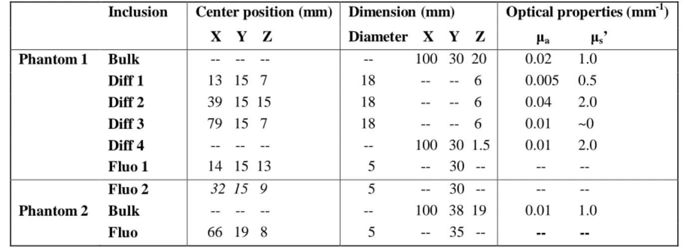
Table 3.1: Optical properties for both phantoms. Phantom 1 and 2 represent the rectangular phantom

and semi-cylindrical phantom, respectively... 37

Table 3.2: CNR of the reconstruction images. CNR1 and CNR2 represent the CNR of the reconstructions with prior and the ones without priors, respectively. ... 50

Table 4.1: Dimension and optical properties of phantom. ... 72

Table 4.2: Four cases of the experiment. ... 73

(17)

LIST OF FIGURES

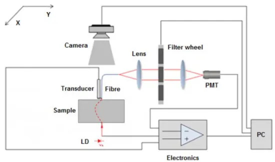
Figure 3.1: Schematic of this dual-modality imaging system. ... 33

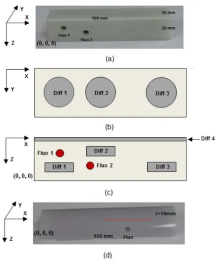
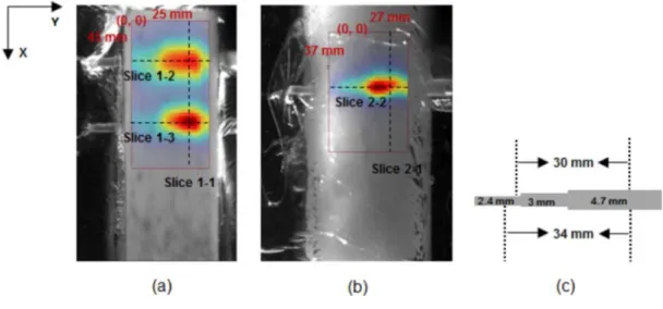
Figure 3.2: (a) Dimension of the rectangular phantom: phantom 1. (b)-(c) Schematic depiction showing the four heterogeneities (denoted by diff 1-4) and two holes for inserting fluorescent tubes (denoted by fluo 1-2). (d) Dimension of the semi-cylindrical phantom, phantom 2. ... 36

Figure 3.3: Illustration of measuring position in the sensitivity test. The red arrows represent the laser diode and the detection fiber. ... 37

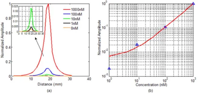
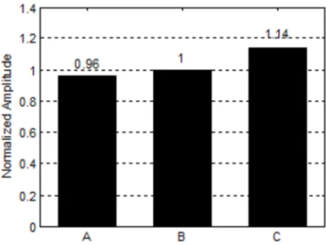
Figure 3.4: (a) normalized values of different concentration as a function of scan position. The results show that the system was able to detect 1nm cy5.5 in the phantom; (b) the curve shows the fitted logarithmic peak values as a function of concentrations. The triangular markers denote the normalized amplitude of different concentrations. ... 38

Figure 3.5: (a) The normalized fluorescence intensity of phantom 1. (b) The normalized fluorescence signal of phantom 2. (c) The dimensions of the plastic tube. ... 40

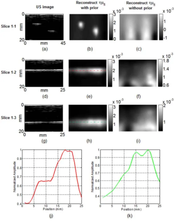
Figure 3.6: Representative images of the acquisition using phantom 1. The US images (a), (d), (g), the fluorescence reconstruction image (ημfl in mm-1) with priors (b), (e), (h), and without priors (c), (f), (i) are shown for image slices at x=20 (a)-(c), at y=14 (d)-(f) and at y=32 (g)-(i) respectively. Intensity plots along the red (j) dashed line in Figure 3.6 (e) and along the green (k) dashed line in Figure 3.6 (h) are also shown. ... 43

Figure 3.7: (a) Overlaid image at x=20. (b) Overlaid image at y=14. (c) Overlaid image at y=32. ... 44

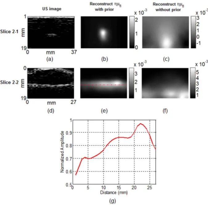
Figure 3.8: Representative images using phantom 2. The US images (a) and (d), the fluorescence reconstruction image (ημfl in mm-1) with priors (b) and (e), and without priors (c) and (f) are shown for image slices at x=12 (a)-(c) and at y=18 (d)-(f). Intensity plot along the red (g) dashed line in Figure 3.8 (e) is also shown. ... 45

Figure 3.9: (a) Overlaid image at x=12. (b) Overlaid image at y=18. ... 46

Figure 3.10: (a) The BN ratio overlaid with the picture. (b) Illustration of the animal manipulation. .. 47

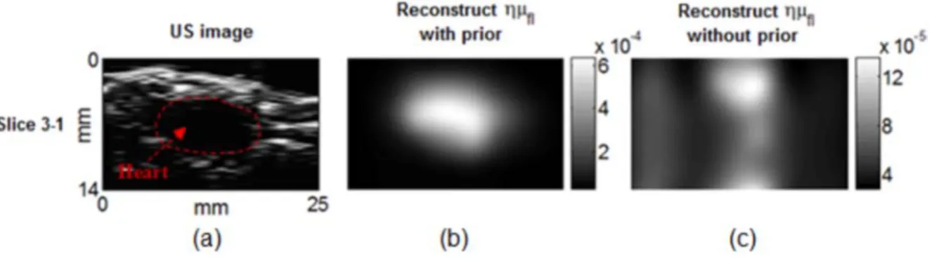
Figure 3.11: Representative images of slice 3-1 of the mouse: (a) The US image shows the heart of the mouse; (b) the fluorescence reconstruction image (ημfl in mm-1) with priors and (c) without... 49

(18)

Figure 3.12: The overlaid image of slice 3-1. ... 49

Figure 3.13: Quantification with the two phantoms by comparing the normalized maximum value of ημfl in each fluorescence image slice. ... 51 Figure 4.1: (a) System schematics of the Fluorescence-US imaging system; (b) photo of the imaging

system; and the window for the scanning of both the laser source and the US transducer is indicated by the yellow square; (c) the scanning window is showed by an enlarged view; and the animal installation is also illustrated. ... 66

Figure 4.2: Illustration of light propagating in tissue. here, r_sandr_drepresents an arbitrary source and

detector position, respectively;lrepresents one effective traveling path of the incident light from

s

r tor_d; l'is a representative travelling path of the incident photons fromr_sto fluorophore;l is a x

representative traveling path of fluorescent photons from the fluorophore tor_d. ... 67

Figure 4.3: Illustration of the phantom and the inclusions. Here, S_a and S_b are the two surfaces of the phantom along the Z direction; F_a and F_b are two holes to insert the fluorescent tubes; D_a and D_b are the two heterogeneous inclusions. ... 71

Figure 4.4: Phantom images for the four cases: the first row shows the ROI for each scan; the second row shows the fluorescence images processed with the standard BN method; the third row shows the standard BN ratio images with only the measurement of the detector co-linear with the source; finally, the fourth row shows the fluorescence images processed with the ACBN method. ... 74

Figure 4.5: Representative image slices. (a) The segmentation of tissue types derived from the combined structural prior; (b) the localization was accurately reconstructed with prior; (c) reconstruction without structural prior. ... 80

Figure 4.6: (a) The true value of εηC only in the tumor region was changed; but the initial estimate was kept constant; (b) the true value of εηC was constant; but the initial estimate was changed; (c) the true values of εηC in both tissue regions were changed; and the value of the tumor region remained 4 times greater than that of the normal tissue region; but the but the initial estimate was kept constant; (d) true values in both tissue-type regions were constant, and the initial estimate was constant too. The reconstructed was assessed with different noise levels. ... 83

(19)

Figure 4.7: The comparison of the reconstruction between the ACBN method and the standard BN method. ... 85

Figure 4.8: As a representative, the tumor is approximately indicated by the dashed circle. ... 85

Figure 4.9: (a) The ROI of imaging was indicated by the red spots; (b)-(c) the fluorescence images acquired before and after injection of the molecular probe for the control; (d)-(e) the fluorescence images acquired before and after injection of the molecular probe for Tumor #1; (f)-(g) the fluorescence images acquired before and after injection of the molecular probe for Tumor #2. .. 87

Figure 4.10: (a)-(c) For Tumor #1, a representative US image slice and two representative fluorescence images overlaid the corresponding US image slices are shown; (d)-(f) For Tumor #2, a representative US image slice and two representative fluorescence images overlaid the corresponding US image slices are shown. ... 89

Figure 4.11: (a) Ex-vivo images of the tumors for Tumor #1 and Tumor #2. The ratio between the maximum reconstructed εηC of Tumor #1 and that of Tumor #2 is 1:0.61; (b) the maximum reconstructed εηC for Tumor #1 and Tumor #2 is shown with the ACBN method as well as the standard BN method. ... 90

Figure 5.1: Schematic (top) and photograph (bottom) of the FMT system. GM: Galvo mirror; EF: excitation fibers; DF: detection fibers; LD: laser driver; FW: Filter wheel... 102

Figure 5.2: Schematic diagram (left, top side) and photograph (right) of the optical probe working in an experiment. AH: animal holder; AP: animal plate; FMR: fiducial marker... 104

Figure 5.3: (a) Representative axial MR slice of ATX #2; (b) segmented image; (c) resampled segmented image with 1 mm voxel resolution. ... 104

Figure 5.4: Schematic diagram of the phantom: (a) view of X-Y plane; (b) view of X-Z plane. The attenuation and fluorescence inclusions are denoted by Diff and Fluo, respectively. ... 107

Figure 5.5: (a) A synthetic fluorescence slice of the phantom; (b) the corresponding slices of the reconstruction with the heterogeneous models (b), and with the homogeneous model (c), respectively; (d) plot of reconstructed values along the red dashed line. (e) CNR was compared with λ for both models. ... 110

(20)

Figure 5.6: (a) Ex vivo images of the fluorescent tubes were overlaid with transparency (alpha=0.5) on the photographs of tubes, respectively; (b) the average reconstructed values (both models) of the fluorescent tubes were normalized of the maximum being 1, to compare with the ex vivo measurement (reference). ... 112

Figure 5.7: (a) Three orthogonal MR slices are shown: axial slice (Y-Z), coronal slice (X-Y) and sagittal slice (X-Z). The arrow of the X axes points to tail of the mouse; and the arrow of the Z axes points to abdomen. The tube was indicated by the red arrow; (b) the reconstructions with the heterogeneous models were overlaid with transparency (alpha=0.5) on the MR slices, respectively; (c) the reconstructions with the homogeneous models were overlaid with transparency (alpha=0.5) on the MR slices, respectively. ... 113

Figure 5.8: The images in the first column are the MR slices for each mouse. Heart and part of aorta of ATX #1 were denoted by red arrows. In the second column, the reconstructed εηC with the heterogeneous models were overlaid with transparency (alpha=0.5) on the MR slices, respectively. Three orthogonal MR slices were chosen for each mouse: axial slice (Y-Z), coronal slice (X-Y) and sagittal slice (X-Z). ... 115

Figure 5.9: The hearts and aortas of the four mice were imaged ex vivo. In the first row, the ex vivo fluorescence images were overlaid with transparency (alpha=0.5) on the corresponding photographs. Shown by the curves below, the average reconstructed εηC of the hearts and aortas for all mice were normalized with the maximum being 1 to compare with the ex vivo measurement. ... 116

(21)

LIST OF ACRONYMS AND ABBREVIATIONS

AFA Angular filter array

BEM Boundary element method

BM Boundary measurement

BN Born-normalization

CNR Contrast to noise ratio

CT Computed tomography

CW Continuous-wave

3D Three dimensional

DFI Diffuse fluorescence imaging

DOT Diffuse optical tomography

EMCCD Electron multiplying charge coupled device

FEM Finite element method

FLI Fluorescence lifetime imaging

FOV Field of view

FMT Fluorescence molecular tomography

GPU Graphics processing unit

Hb Deoxy-hemoglobin

HbO2 Oxy-hemoglobin ICG Indocyanine green

MC Monte Carlo

MEMS Microelectromechanical systems MicroCT Microcomputed tomography

(22)

MRI Magnetic resonance imaging

MMP Matrix metalloproteinases

PAT Photo-acoustic tomography

PCA Principal component analysis

PET Positron emission tomography

PMT Photomultiplier tube

PpIX Protoporphyrin IX

ROI Region of interest

RTE Radiative transfer equation

SNR Signal to noise ratio

TR Tikhonov regularization

US Ultrasound

,

s

µ

Reduced scattering coefficient

a

(23)

CHAPTER 1 GENERAL CONTEXT

1.1 Overview

Diffuse Fluorescence Imaging (DFI) has been widely used in biological, preclinical and

clinical studies because of its excellent sensitivity and specificity (Gibson, Hebden, & Arridge,

2005; Frederic Leblond, Davis, Valdés, & Pogue, 2010; Frederic Leblond, Tichauer, Holt,

El-Ghussein, & Pogue, 2011). With the administration of an exogenous fluorescent molecular probe,

receptors expressed during a given disease could be targeted. In some cases, enzymes can

activate a probe to fluoresce, specifically expressing the activity of the targeted molecules (H. H.

Chen et al., 2013; Jaffer, Libby, & Weissleder, 2009a; Ripplinger et al., 2012; Sanz & Fayad,

2008; Tardif, Lesage, Harel, Romeo, & Pressacco, 2011; Vries et al., 2009). In both cases, the

fluorescent molecules act as an antenna: after being excited, the fluorescent photons escaping

from the tissue can be detected on the boundary of the tissue by a fluorescence imaging system.

To quantify the received fluorescence, these boundary measures will be taken as input for a

model-based 3D fluorescence reconstruction (Gibson et al., 2005). Following this modeling, with

the reconstruction algorithm, fluorescent concentration can be quantified and localized, thereby,

revealing the molecular activities in the progression of the disease (Markel, Mital, & Schotland,

2003).

In Fluorescence Molecular Tomography (FMT), light within the wavelength range 650

nm to 800 nm is typically employed in the form of collimated beam or wide-field patterns to

excite the fluorophores in a given sample (Ntziachristos, Bremer, & Weissleder, 2003). The

reason is that within this range of wavelengths, the main absorbers in tissue, e.g.

(24)

allows deeper penetration in tissue and enable signal detection with better signal to noise ratio

(SNR) (S. A. Prahl, n.d.; L. V. Wang & Wu, 2007).

In contrast to microscopic imaging techniques, FMT belongs to the regime of

macroscopic diffuse light imaging and provides millimeter-level spatial resolution, but preserves

the ability to image up to several centimeters deep in tissue (L. V. Wang & Wu, 2007). Distinct

from anatomical imaging modalities, such as X-ray computed tomography (CT), magnetic

resonance imaging (MRI) and ultrasound (US), it yields functional information about the

biological processes or activities of disease-related molecules (Ntziachristos et al., 2003).

Furthermore, when compared to ionizing imaging techniques, such as contrast enhanced X-ray

CT or positron emission tomography (PET) (Fu et al., 2013; Nahrendorf et al., 2010; Ricketts,

Guazzoni, Castoldi, Gibson, & Royle, 2013), FMT is non-ionizing, thus, does not create a risk

for subjects with the imaging tasks. Therefore, given its simplicity and low-cost, FMT may have

great potential in biological and preclinical/clinical applications.

Depending on the excitation mechanism, fluorescence imaging can be divided into

frequency-domain, continuous-wave (CW) and time-domain fluorescence imaging (L. V. Wang

& Wu, 2007). In the frequency-domain, the excitation light wave is modulated with a high

frequency (e.g. 100MHz) and the measurement consists of both amplitude and phase information

of the emitted photons. However, CW mode is a special case of the frequency-domain with

modulation frequency set to zero. In this case the measurement only contains amplitude

information. In the time-domain technique, a pulsed laser is typically used to excite the

fluorophore and the emitted photons are recorded by a time-gated camera or photon-counting

device. The frequency-domain and time-domain are more complex than the CW technique in

(25)

and lifetime of the injected fluorophores in tissue. However, the CW system has advantages in

low-cost, easy implementation, and fast acquisitions. Beyond these three modes, recently efforts

in optimizing the illumination spatial pattern were done. A spatial domain frequency method was

reported in several studies, e.g. to resolve optical properties in tissue (Weber et al., 2011) as well

as enhance resolution and contrast of fluorescence imaging (Mazhar et al., 2010).

In the next sub-chapter, different aspects of FMT will be introduced by briefly reviewing

the recent literature. The versatility of the fluorescence imaging tools will first be reviewed for a

variety of applications. Second, FMT, or in general, diffuse fluorescence imaging

instrumentation will be summarized using recent studies. Then, the latest development of

hybrid-modal FMT and its advantages will be briefly reviewed. Finally, we will review the

computational progress in FMT, including both forward and inverse problems as well as the data

calibration techniques.

1.2 Brief literature review

Diffuse fluorescence imaging, in general, has been mainly used in preclinical and

biological studies. Several studies in-vivo were conducted showing that lymphatic function could

be evaluated by monitoring the fluorescence signal in the micro-circulation following the

administration of indocyanine green (ICG) (Kwon, Agollah, Wu, Chan, & Sevick-Muraca, 2013;

Kwon & Sevick-Muraca, 2011; Solomon et al., 2011). The results suggested that by imaging

fluorescence in lymphatic nodes, lymphatic architecture could be visualized and the progression

and metastasis of cancer might be staged. Until now, tumorous/cancerous imaging remains one

of primary applications with fluorescence imaging. Using wide-field fluorescence lifetime

imaging (FLI), surface tumors could be detected by auto-fluorescence imaging of the skin at Applications

(26)

video-rates (McGinty et al., 2010). In other studies, fluorescence imaging combined with other

imaging techniques or working alone were employed to characterize tissue properties for the

diagnosis of skin cancer (Dancik, Favre, Loy, Zvyagin, & Roberts, 2013; Gruber et al., 2010a;

Nie, An, Hayward, Farrell, & Fang, 2013; Sunar, Rohrbach, Morgan, Zeitouni, & Henderson,

2013). These studies suggest a great potential of translation to humans for biopsy of cancerous

tissue. Fluorescence imaging was also employed to characterize brain tumors by using

near-infrared dyes (Davis et al., 2010; Fortin et al., 2012). The biophysics underlying these

applications is that lesions and normal tissues will show distinctive characterizations with respect

to the accumulation and metabolism of the fluorescent dye reflected by different levels of

fluorescent signal intensity and pharmacokinetic rate. Using this principle, tumor neo-vasculature

was measured by dynamic fluorescence imaging (M. Choi, Choi, Ryu, Lee, & Choi, 2011); and

tumor contrast was obtained by late-fluorescence mammography aiming to separate malignant

lesions by assessing tumor capillary permeability (Hagen et al., 2009). Furthermore, fluorescence

imaging was employed intraoperatively to delineate lesion (tumor) margins (Q. Zhao, Jiang, et

al., 2011) or to guide the concurrent surgery (Themelis, Yoo, Soh, Schulz, & Ntziachristos,

2009). It has been argued that the spectroscopic information measured during fluorescence

imaging could aid in the diagnosis of many other carcinomatous diseases, such as oral cancer

(Fatakdawala et al., 2013), glioma tumors in the brain (Gibbs-Strauss et al., 2009), prostate

cancer (Boutet et al., 2009) and pancreatic cancer at early stage (Erten et al., 2010). Fluorescence

imaging was also demonstrated using tomographic approaches to quantify and localize tumors

(Ale, Ermolayev, Deliolanis, & Ntziachristos, 2013; Deliolanis et al., 2009; D. S. Kepshire et al.,

(27)

such as hybrid modalities, single photon detection and complete-angle projections were explored

to retrieve the functional information associated with cancer.

Cardiovascular imaging is another major application of fluorescence imaging.

Spectroscopic measures were used to characterize atherosclerotic plaques using time or

wavelength resolved detection methods (Larsen et al., 2011; Liu, Sun, Qi, & Marcu, 2012;

Sćepanović et al., 2011; Yinghua Sun et al., 2011). Fluorescence imaging was also used to guide surgery for cardiovascular disease (Cooley, 2011). Moreover, as cardiovascular tissue exhibits

high absorption due to the enriched blood content, in-vivo atherosclerotic imaging was mainly performed in the form of endoscopy (Bec et al., 2012; Calfon, Vinegoni, Ntziachristos, & Jaffer,

2010; Mallas et al., 2012; Razansky et al., 2010; Xie et al., 2012). In these studies, catheter

probes were used to accommodate a fluorescence detector or coupled with additional US transducers to visualize intravascular vessels and characterize atherosclerotic plaques. One in-vivo study reported autophagy imaging in the heart using FMT by recovering cathepsin activity

(H. H. Chen et al., 2013). However, until now, very few examples for non-invasive in-vivo

atherosclerosis imaging exist. Developing such examples is one of the focus point of this thesis. Beyond diagnosis, fluorescence imaging also contributed to assess therapy. It was reported that time-domain and spatial frequency domain fluorescence imaging could quantify fluorophore distribution in order to assess photodynamic therapy (Mo, Rohrbach, & Sunar, 2012;

Saager, Cuccia, Saggese, Kelly, & Durkin, 2011). In radiotherapy, Cerenkov emission was used

to excite fluorescent molecular reporters; ensuing fluorescence mapping could potentially evaluate and monitor tissue response of therapy (Axelsson, Davis, Gladstone, & Pogue, 2011;

Demers, Davis, Zhang, Gladstone, & Pogue, 2013). Other examples using FMT include the

(28)

fluorescence techniques enabled pH sensing with biological samples as well as in small animals

(Hight et al., 2011; J. Li et al., 2012). Dynamic FLI was used to assess protein-losing

nephropathy due to renal diseases (Goiffon, Akers, Berezin, Lee, & Achilefu, 2009). A

proof-of-concept study demonstrated the feasibility of employing time-resolved dynamic imaging of ICG

to provide information on the blood supply to the brain of humans (Milej et al., 2012);

parameters related with imaging geometries and fluorophore wavelength were optimized for

imaging amyloid plaques with Alzheimer's disease mice (S B Raymond, Kumar, Boas, &

Bacskai, 2009).

Many of the examples introduced above were also extended to humans. In the study of

carcinomatous disease, fluorescence imaging combined with diffuse optical tomography (DOT)

was employed to measure the pharmacokinetic rate of ICG to discriminate malignant lesions

from normal tissue in the human breast (Leproux et al., 2011). Malignant tissue in the human

breast could also be distinguished from healthy tissue by measuring deoxy-glucose using

wide-field fluorescence imaging (Langsner et al., 2011). In the same application, integration between

DOT and time-resolved fluorescence was used to recover optical properties and fluorescent

properties towards a comprehensive diagnosis for breast cancer (W. Zhang et al.,

2013)(Grosenick et al., 2011). A hand-held fluorescence imaging scheme was proposed and

expected to translate into clinical studies (Erickson et al., 2013; Ge, Erickson, & Godavarty,

2010; J, Sj, & A, 2009). Ex-vivo fluorescence imaging was also enabled by activatable molecular

probes: multispectral FMT was employed to reveal matrix metalloproteinases (MMPs) activities

in the characterization of human carotid plaque (Vries et al., 2009). Multimodal FLI was used to

characterize the composition, structure and function of human atherosclerotic plaques ex-vivo

(29)

surgery. Here, a ratiometric fluorescence approach could result in a better delineation of tumor

boundary in image guided surgery (F Leblond et al., 2011). This maneuver might even be

achievable by a pulsed light excitation fluorescence imaging method to perform surgery under

normal room lighting (Sexton et al., 2013).

The applications discussed above demonstrate the versatility of fluorescence as well as

the efforts in this field for the development of different aspects. In this sub-section, recent

instrumental and methodological advancements of fluorescence imaging will be concisely

introduced. Multi-modal imaging and computational developments, such as forward/inverse

problems and data calibration techniques will be introduced in the next two sub-sections. General development of fluorescence imaging

Fluorescence imaging can be performed in different geometries. In epi-illumination mode,

both illumination and detection are conducted on the same side of sample. In trans-illumination

mode, illumination and detection are conducted on the separate sides of the sample. The former

is sensitive to depth, but has limited penetration of light in tissue; and it is less immune to

auto-fluorescence contamination. An all optical approach was developed that by dynamically

measuring reflectance ICG signal, tissue anatomy could be revealed due to the distinctive

pharmacokinetic rate of different tissue types (Hillman & Moore, 2007). It was reported recently

that the Mellin-Laplace transform of time-domain reflection data could potentially help probe

deep inclusions (Puszka et al., 2013). The transmission measures are less sensitive, but have

better ability to detect objects embedded deeply, which would suggest a better SNR for

measurements. For example, transmission fluorescence was employed to image biocompatible

upconverting nanoparticles embedded in mice, which demonstrated an auto-fluorescence free

(30)

working in the angular domain might decrease scattering effect to detect deep objects in mice

(Vasefi et al., 2009). Here, angular domain refers to a technique using the angular filter array

(AFA) to overcome to collect emission photons going through limited scattering events. A more

advanced approach is to acquire projection measurement over 360o around the imaging sample, which is expected to combine the merits of both reflection and transmission. Investigators

combined both FMT and X-ray CT to acquire projection dataset in both modalities for animal

studies in-vivo (Ale et al., 2012a; Ale, Schulz, Sarantopoulos, & Ntziachristos, 2010; Lapointe,

Pichette, & Bérubé-Lauzière, 2012).

Besides imaging geometries, the development of detection mechanisms and illumination

methods also had significant impact on the imaging performance. It has been broadly reported

that time-domain could provide superior information in term of richness of information over

CW-mode fluorescence imaging (Holt, Tichauer, Dehghani, Pogue, & Leblond, 2012). Instead of

measuring optical intensity like the CW-mode does, time-domain measurement has temporal

resolution up to hundred picoseconds, which could result in the recovery of lifetime of

fluorophore. Different from CW intensity measures, lifetime measures are immune to

experimental and biological factors, such as laser power, probe uptake and concentration

(Goergen, Chen, Bogdanov, Sosnovik, & Kumar, 2012). The benefits of time-domain have been

proven by theoretical studies (Ducros, Da Silva, Hervé, Dinten, & Peyrin, 2009; Ducros, Hervé,

Da Silva, Dinten, & Peyrin, 2009). One of the appealing features of time-domain schemes would

be to reconstruct or separate fluorescence yield and the lifetime of endogenous fluorophores

(Gao et al., 2010; Nothdurft et al., 2009). And the contrast to background of lifetime measures

could even be enhanced when employing a fluorophore having a distinct lifetime from the auto-fluorescence (May, Bhaumik, Gambhir, Zhan, & Yazdanfar, 2009). A time-gated method was

(31)

used to record the arrival time of photons. So, depending on arrival time of selected photon, the

depth of fluorescent object could be resolved (Q. Zhao, Spinelli, et al., 2011). Other studies

demonstrated in simulation and experiments that using early arriving photons could reduce the scattering effect in the detection, thereby yielding significant improvements in the quality of fluorescence reconstructions (Niedre & Ntziachristos, 2010; B. Zhang et al., 2011; Q Zhu et al.,

2011). Further studies using early arrival photons showed that multiple point-like fluorescent

inclusions could be separated with millimeter spatial error; and both spatial resolution and image contrast were improved. These conclusions were verified by simulation and phantom experiment

(Pichette, Domínguez, & Bérubé-Lauzière, 2013). Another advantage of time-domain technique

is lifetime multiplexing due to the distinct lifetime decay profiles of different fluorophores. This

technique was demonstrated both in phantoms and mice in vivo (J. Chen, Venugopal, & Intes,

2011; Scott B Raymond, Boas, Bacskai, & Kumar, 2010; Rice, Hou, & Kumar, 2013). Lifetime

measurements could also be achieved by the frequency-domain modality, using the detected

intensity and phase information (Chatni, Li, & Porterfield, 2009; DiBenedetto, Capelle, &

O’Neill, 2012; Elder, Kaminski, & Frank, 2009; Y Lin et al., 2011a). However, either

time-domain or frequency-time-domain suggests implementation complexity, long acquisition and

relatively high cost. Strategies have been developed in order to preserve low cost, fast acquisition

and good performance. Illumination strategies were developed aiming to shorten acquisition time

while preserving informative datasets. Line excitation was compared with point or area

illumination and phantom and animal experiments showed it as a feasible illumination scheme to

potentially achieve quantitative recovery of fluorescence (L. Cao & Peter, 2013; D. Wang, Liu,

& Bai, 2009). Wide-field excitation was adopted in time-domain fluorescence to reconstruct

(32)

Abe, Barroso, & Intes, 2013). Low modulation frequency and LED illumination was used to

achieve an alternative solution for FLI (Gioux, Lomnes, Choi, & Frangioni, 2010). In one

example, a function generator was used to modulate a laser diode; thereby, the frequency-domain

mechanism became cost efficient (B. Yuan, McClellan, Al-Mifgai, Growney, & Komolafe,

2009). In this sense, the CW-mode technique could be a good compromise between performance

and cost (Patel et al., 2010). Further studies showed that early photons detection suffered from a

low SNR due to the rejection of a great amount of emitted light; hence, first reconstructing with

the quasi-CW data and then refining with early photons measurements were shown to yield a

better resolution of fluorescence reconstruction image (Z. Li & Niedre, 2011). More recently, a

spatial-frequency domain system was developed. In this technique, a low-cost projector was used

to spatially modulate the CW excitation light for detecting both spatial frequency and intensity

information. Demonstrated in a phantom study, illumination patterns with multiple spatial

frequencies were projected on the surface of the imaging object; the depth recovery of

fluorescent objects could be achieved by varying the spatial modulation frequency (Mazhar et al.,

2010). Spatial-frequency fluorescence acquisition was conducted in tomographic mode with

rotating view (Ducros et al., 2013). Both theoretical and experimental studies have been

conducted to optimize illumination patterns to exploit the illumination flexibility as well as

reduce computation burden (Dutta, Ahn, Joshi, & Leahy, 2010; Ducros et al., 2010; Ducros,

D’Andrea, Bassi, Valentini, & Arridge, 2012). Arguably, using Cramer-Rao theoretical analysis,

it was stated that the best depth precision of fluorescent object with FLI was not significantly

better than the spatially modulated CW technique (Boffety, Allain, Sentenac, Massonneau, &

(33)

Additionally, multi-spectral approaches have been explored to increase the measurement

dimension in the wavelength domain. First, simulation work was conducted to validate the

feasibility of employing multispectral excitation for a quantitative fluorescence reconstruction

(Chaudhari et al., 2009). And it was reported that multispectral excitation might be able to

separate different fluorophores having different concentrations (Pu et al., 2013). Using a tunable

wavelength selection device, hyper-spectral excitation was achieved (Klose & Pöschinger, 2011).

The development of fluorescence imaging was also motivated by precision machining and fabrication. For example, investigators used (angular filter array) AFA to overcome the

effect of scattering in macroscopic fluorescence imaging. By the AFA, only the emitted photons going through minimal scattering events would be collected; as a result, the retrieved fluorescence mapping could be enhanced to sub-millimeter resolution (Najiminaini et al., 2010;

Vasefi et al., 2009; Vasefi, Belton, Kaminska, Chapman, & Carson, 2010). Separately, a

handheld fluorescence imager probe consisting of micro-electromechanical systems

(MEMS)-based scanning mirror was developed. And its ability for 3D fluorescence tomography was

evaluated in in-vivo imaging of small animals (He et al., 2012). Moreover, another study

reported that a micro-lensed dual-fiber optical probe would largely improve the detection efficiency of light, hence, result in a better SNR of measurement (H. Y. Choi et al., 2011).

These state-of-the-art techniques have also been pursed to work in conjunction with

complementary anatomical imaging modalities, such as MRI, X-ray CT, and US. The benefits of

this combination are multiple and improvements significant. In one instance, photo-acoustic

tomography (PAT) was combined with FMT, thus the high resolution of PAT and high

sensitivity of FMT could be correlated to for a comprehensive pathological analysis (B. Wang, Multi-modality fluorescence imaging

(34)

Zhao, Barkey, Morse, & Jiang, 2012). A clinical study was conducted to reconstruct oxygen

saturation and water content of joint tissues to separate osteoarthritic joints from healthy ones in

the hand. In this study, the physiological parameters were recovered guided by the X-ray CT

images (Z. Yuan, Zhang, Sobel, & Jiang, 2010). Likewise, a fluorescence probe coupled with

transrectal US was used on a prostate phantom, and demonstrated its feasibility on guiding

biopsies of tumors (Laidevant et al., 2011). Also, US images were used to provide anatomical

prior information in white light excited fluorescence imaging; the recovered protoporphyrin IX

(PpIX) mapping was capable of evaluating photodynamic therapy for human skin tumor (Flynn,

DSouza, Kanick, Davis, & Pogue, 2013). A handheld fluorescence imager combined with an

acoustic sensor was able to detect small fluorescent objects deep in a phantom, as well as

determine imager orientation and phantom geometry (Erickson, Martinez, Gonzalez, Caldera, &

Godavarty, 2010).

Several studies showed that the prior information recovered from anatomical images

could improve the quality of reconstructions in terms of quantification and localization. X-ray

images were used to provide prior information to determine optical properties for

bioluminescence tomography (Naser & Patterson, 2010a). Similar work showed that X-ray CT

images provided anatomical guidance for FMT; and the image accuracy was improved even

when using limited projection scans for FMT (Radrich, Ale, Ermolayev, & Ntziachristos, 2012).

Microcomputed tomography (MicroCT) was also employed to couple with single photon counting FMT for small animal imaging; and with CT image guidance, PpIX was accurately

recovered from mouse phantoms (D. Kepshire et al., 2009). Beyond anatomical priors, other

studies showed that PET functional priors, which were also specific to a lesion, could improve fluorescence reconstruction when using targeted molecular fluorescent probe (C. Li, Wang, Qi,

(35)

& Cherry, 2009). Likewise, optical properties could be reconstructed by CW DOT; subsequently,

the simulation of photons propagation could be optimized for a better fluorescence

reconstruction (Naser & Patterson, 2010).

Tri-modality imaging appears as a more sophisticated imaging strategy. Herein, a

commercial microPET/CT was integrated with frequency-domain fluorescence imaging and

employed with small animals to image fluorescent agent targeting on orthotopic growth of

human prostate cancer (Darne et al., 2012). Also, the combination of MRI, DOT and FMT could

provide anatomical and functional priori information for an improved fluorescence

reconstruction. In this last study, MRI anatomy guided the recovery of optical properties of tissue.

Then both the anatomical and functional information helped recover a fluorescent inclusion

embedded 15 mm deep in rat with less than 5% quantification error (Yuting Lin, Ghijsen,

Nalcioglu, & Gulsen, 2012). Another study demonstrated that with both X-ray CT anatomy and

DOT functional information, fluorescence could be quantitatively recovered. An in vivo

evaluation showed quantification errors as low as 2% (Yuting Lin et al., 2010b).

As FMT process involves model-based reconstruction, the developments of forward

modeling and the inverse problem are critical in this diffuse light imaging technique. The

forward modeling is the process describing photons propagation in tissue and linking the

variation of optical/fluorescent properties of tissue to individual sources or detectors. Monte

Carlo (MC) is one of the most commonly used methods to simulate photons propagation. A MC

program was presented in 1995, to simulate photons traveling in tissue with multi-layer structure.

High agreement was reached with analytical diffusion models (L. Wang, Jacques, & Zheng,

1995). Following, the tMCimg algorithm was proposed to simulate photons in tissues having Reconstruction, data extraction and calibration

(36)

complex 3D geometry (Boas, Culver, Stott, & Dunn, 2002). More recently, meshed based MC

was developed, which displayed an accuracy comparable to analytical diffuse models for targets

with curved boundaries (Fang, 2010). A direct MC algorithm was also reported that stored

photons traveling paths and then showed that fit between fluorescent properties and tissue

absorptions could be completed rapidly (Kumar, 2012). In addition to MC, radiative transfer

equation (RTE) derived forward modeling was also broadly employed in fluorescence

reconstruction. Several studies showed its accuracy and agreement with MC (Liemert & Kienle,

2012; Montejo, Klose, & Hielscher, 2010). To simplify the RTE in terms of complexity and

computation time, the diffusion equation has also been commonly used. DE is the first order

angular approximation to the RTE under an approximation that

µ

_s, >>

µ

_a, which is true when light travels a few millimeters in tissue but less accurate close to boundaries. In one study, an

additive correction was added to the DE; and substantial improvements were shown in

comparison to standard DE (Lehtikangas, Tarvainen, & Kim, 2012). Another way to improve the

DE was to combine both RTE and DE. Specifically, DE was replaced with RTE in the spatial

regions where the modeling accuracy increased (Gorpas & Andersson-Engels, 2012). Other

high-order approximations of RTE were also explored and the improvement of modeling

precision was observed comparing with the standard DE (Lu et al., 2010).

The inverse problem aims to retrieve the fluorescence properties, given the weight matrix

found by the forward modeling and the experimental measurements. Since inversion involves

taking the inverse of the weight matrix, the inverse computation is unavoidably ill-posed, thus is

commonly resolved iteratively. Tikhonov Regularization (TR) is regarded as one of commonly

used techniques in fluorescence reconstruction (Arridge & Schotland, 2009). Specifically in

(37)

objective function as a penalty term to constrain the optimization process (Yalavarthy, Pogue,

Dehghani, & Paulsen, 2007). In addition to the L2 norm that is often used to integrate the prior in

TR, other methods have been investigated to better utilize the prior for fluorescence

reconstruction. The L1 norm was suggested as a penalty term to regularize the reconstruction,

and it was shown that it gave sparse solutions and could avoid the over-smoothing effects

particularly when solving sparsely localized small fluorescent objects (Basevi et al., 2012;

Chamorro-Servent et al., 2013; Kavuri, Lin, Tian, & Liu, 2012; Q. Zhang, Chen, Qu, Liang, &

Tian, 2012). A total variation regularization was proposed showing its advantages over the L2

norm of avoiding over-smoothness and enhancing the spatial resolution of fluorescent object in

the reconstruction fluorescence images (J F P-J Abascal et al., 2011; Behrooz, Zhou, Eftekhar, &

Adibi, 2012; Freiberger, Clason, & Scharfetter, 2010). A joint L1-total variation norm was seen

to have the advantages of preserving the edge and the local smoothness (Dutta, Ahn, Li, Cherry,

& Leahy, 2012). In all these techniques, the regularization parameter is also a subtle but

important point to adjust the strength of the penalty term. Here, a L-curve method was often used,

with which the regularization parameter would be determined at the corner of the log-log plot of

the regularized solution and the norm of the corresponding residual (Hansen & O’Leary, 1993).

Also, it was demonstrated that a U-curve method could be used to select the regularization

parameter in the reconstruction of DFI (Chamorro-Servent, Aguirre, Ripoll, Vaquero, & Desco,

2011). Instead of these automatic methods, an optimal value of regularization parameter was

often determined empirically (Yalavarthy, Pogue, Dehghani, & Paulsen, 2007).

Given a well-developed reconstruction algorithm, data of good quality is expected to

bring good results. In this sense, data calibration can be used to cancel off experimental factors,

(38)

been widely applied in fluorescence imaging, by which the ratio between fluorescent signal and

intrinsic light signal is taken as input for the reconstruction. With this approach, experimental

factors, such as laser power and coupling loss can be cancelled (Ntziachristos & Weissleder,

2001). In another study, a workflow of calibration steps was elaborated for a CT-guided FMT

system. The phantom results indicated the importance of careful calibration (Tichauer et al.,

2011). When guided by anatomical image, the sampling of problematic data could be reduced;

thus the fidelity of reconstruction was improved (X. Zhang et al., 2011). Also, work was done to

reduce the image artifact due to tissue heterogeneity. In one study, fluorescence from the targeted

lesion was corrected by an excitation image to reduce the artifact induced by the spurious

fluorescent signal because of the parts of tissue that was thin or had low-absorption (Mohajerani,

Adibi, Kempner, & Yared, 2009). Fidelity of measurements can also be enhanced experimentally.

In one study, specific fluorescence signal was subtracted from an unbounded surrogate. This

dual-tracer approach reduced the background signal originated from the bounded probe; thereby

demonstrating substantial improvement in image contrast (Tichauer et al., 2013). Furthermore,

good acquisition means having of a high SNR. In this endeavor, automatic control of imaging

exposure time helps avoid saturation for the thin tissues, and enable high signal amplitude for the

absorbing portions, ultimately to ensure linearity of measurement (D. L. Kepshire, Dehghani,

Leblond, & Pogue, 2009). In fluorescence imaging, excitation light leakage contaminates the

fluorescence signal. To overcome this, the combination between appropriate filter and

collimation optics could efficiently reject excitation light thus potentially improve the detection

sensitivity of fluorescence (B. Zhu, Rasmussen, Lu, & Sevick-Muraca, 2010).

Methods have been investigated to speed up the computation for both forward modeling

(39)

method (FEM) computational approach simplified the nodes for outer tissue but kept the

complexity for the internal ones. And the computational speed using this approach was shown to

be faster than the standalone FEM (Srinivasan, Ghadyani, Pogue, & Paulsen, 2010). The size of

the forward model matrix could be compressed by wavelet methods whilst preserving the

significant information (Correia, Rudge, Koch, Ntziachristos, & Arridge, 2013; Ducros et al.,

2011). In a separate study, the wavelet method was applied to reduce model dimension in order

to speed up the computation (Landragin-Frassati, Dinten, Georges, & Da Silva, 2009). Principal

component analysis (PCA) methods were also used to reduce measurement redundancy for a fast

and informative reconstruction (X. Cao et al., 2013; Mohajerani & Ntziachristos, 2013). Along

the same line, a fast reconstruction was achieved by an iterated shrinkage based reconstruction

method with sparsity regularization, showing accurate results with limited measurement data

(Han et al., 2010).

Fast computations could also be achieved by advanced programming techniques. A

matrix-free technique was developed using a Matlab function, called ‘gmres’, to optimize the

objective function, in which the creation and storage of big Jacobian matrices were avoided, thus

computation burden reduced (Zacharopoulos et al., 2009). Different studies demonstrated that

the graphics processing unit (GPU) based parallel computing could largely shorten the

computation in a MC based forward modeling (Fang & Boas, 2009), as well as for both forward

modeling and inverse problem in a DE based scheme (Freiberger, Egger, Liebmann, &

Scharfetter, 2011).

1.3 Organization of the thesis by objectives

(40)

Objective #1:

• Hypothesis #1-1: The fluorescent and structural information recorded from the fluorescence-US system could benefit the extraction of fluorescent functional

information.

To develop a low-cost multi-modality imaging system combining CW

transmission fluorescence imager and home-made single-element-transducer US system.

Proof-of-concept study was conducted to characterize the system and assess its feasibility

for in-vivo animal imaging.

• Hypothesis #1-2: This low-cost combined system could potentially provide an imaging strategy for in-vivo study with mice.

The article that addressed this objective is:

Baoqiang Li, Maxime Abran, Carl Matteau-Pelletier, Léonie Rouleau, Tina Lam, Rishi Sharma,

Eric Rhéaume, Ashok Kakkar, Jean-Claude Tardif and Frédéric Lesage, "Low-cost

three-dimensional imaging system combining fluorescence and ultrasound," J. Biomed. Opt. 16,

126010 (Dec 06, 2011).

Objective #2:

•

The second objective was to improve the fluorescence-US system in

terms of sampling precision and reconstruction mechanism. The system would further be

validated using in-vivo molecular imaging with tumorous murine model.

Hypothesis #2-1:

•

An electron multiplying charge coupled device (EMCCD) camera

detection will enrich the recording of fluorescent emission. The US subsystem and

the profilometer will provide accurate structural information of the imaging sample.

Hypothesis #2-2:

This fluorescence-US system can serve as a potent tool for

(41)

Baoqiang Li, Romain Berti, Maxime Abran and Frederic Lesage, “Ultrasound guided

fluorescence molecular tomography with improved quantification by an attenuation compensated

born-normalization and in vivo preclinical study of cancer,” Rev. Sci. Instrum., vol. 85, no. 5, p.

053703 (May 2014).

Objective #3:

•

Develop a MRI-guided FMT system for atherosclerotic imaging with

mice.

Hypothesis #3-1:

•

MRI anatomy can help optimize the forward modeling for 3D

fluorescence reconstruction.

Hypothesis #3-2:

This multi-modality imaging approach can achieve quantitative

fluorescence reconstruction for atherosclerotic studies with mice.

Baoqiang Li, Foued Maafi, Romain Berti, Philippe Pouliot, Eric Rhéaume, Jean-Claude Tardif,

and Frederic Lesage, "Hybrid FMT-MRI applied to in vivo atherosclerosis imaging," Biomed.

Opt. Express 5, 1664-1676 (2014).

The thesis is planned as follows: In the second chapter, the basic theory of diffuse

fluorescence imaging is described, which includes the concepts of forward modeling, inverse

problem, as well as how to reconstruct fluorescence targets from boundary measurement (BM).

From the third chapter to the fifth chapter, three published papers are presented addressing the

objectives above. In these three chapters, DFI was first incorporated with US imaging, and then

MRI. The benefits of these anatomical modalities were evaluated by simulation, phantoms and

mice experiments in vivo. In the sixth chapter, a discussion of the advantages as well as

limitations of the proposed multi-modality imaging approaches is discussed. Finally, the thesis is

(42)

CHAPTER 2 THEORY OF DIFFUSE FLUORESCENCE IMAGING

The theory behind Diffuse Fluorescence Imaging (DFI) consists of forward modeling and

solving the inverse problem (Arridge & Schotland, 2009; L. V. Wang & Wu, 2007). The former

predicts how the photons propagate through tissue with known optical properties of tissue,

source/detector positions, as well as power and direction of illumination. The outcome of the

forward modeling is a weight matrix. The latter is then used to reconstruct the fluorescent/optical

properties from BM based on this same weight matrix which may be iteratively modified during

this process. When linearizing the system, a simplified description of fluorescence reconstruction

can be modeled by:

AX

Y = (2.1)

where Y represents the experimental measurements; X is the fluorescent properties to be

reconstructed; A is weight matrix. Having the measurement, X could be reconstructed by

inversing the weight matrix A:

Y A

X = −1 (2.2)

The inverse of the matrix A is often ill-posed and computationally demanding to compute. Hence,

sophisticated method has been developed to reduce the ill-posedness of the inverse problem.

Furthermore, for accuracy, the forward modeling needs an accurate geometrical

definition of the problem domain. This requirement motivates the incorporation with

supplemental anatomical imaging modality. As an added bonus, the anatomical images can also

be used to regularize the fluorescence reconstruction.

2.1 Forward modeling

Several methods exist to simulate the photons propagation in biological tissue. MC

(43)

Boas, 2009; Boas et al., 2002). The eventual evaluation of a given process is estimated with

averaging multiple independent photons. The RTE method models photons transport analytically

(Gorpas & Andersson-Engels, 2012). Because of its complexity, it is often simplified to the DE

under the approximation of

µ

_s, >>

µ

_a. The DE method is less accurate in comparison to MC and RTE, but computationally efficient, therefore, has been widely adopted in simulating photons

propagation.

In this subchapter, the forward modeling will be strictly based on the DE in the CW mode.

Nonetheless, the concepts, such as Green function, weight matrix can be translated to other

modeling methods. Please refer to other materials (Arridge & Schotland, 2009; Dehghani et al.,

2009; Markel et al., 2003; L. V. Wang & Wu, 2007) for a detailed equation derivation and

comprehensive understanding of forward modeling.

The fluorescent photons propagation in diffusive medium can be described by the

following coupled diffusion equations. Under the principle of red-shift (L. V. Wang & Wu,

2007), the fluorophore embedded in medium absorbs photons at the wavelength ofλ_x; and then emits fluorescence at wavelengths greater thanλ_x, λ_m. Because optical properties (

µ

_s,andµ_a) are wavelength dependent, the photon propagation in medium is described by the following two

equations: ) , ( ) , ( ] ) ( [ ) , ( ) (r U r ω c cµ r iωU r ω q r ω Dx ∇ x + ax + x = ⋅ ∇ − _(2.3) 2 )] ( [ 1 ) ( 1 ) , ( ) ( ) ( ) , ( ] ) ( [ ) , ( ) ( r r i r U r r r U c i r r U r D_m _m _am _m _fl _x

ωτ

ω

µ

η

ω

µ

ω

+ − = + + ∇ ⋅ ∇ − (2.4)

where the subscripts x and m represent excitation wavelength and emission wavelength,

respectively; ris a random position in the imaging medium Ω; ω is modulation frequency, which equals to zero in the CW mode. The termU(r,ω)represents the photon density;µ_a(r)is the

(44)

optical absorption coefficient; )) ( ) ( ( 3 1 ) ( _, r r r D s a µ µ +

= is the diffusion coefficient with

µ

,_s(r)

representing the reduced scattering coefficient; τ and η are the lifetime and quantum yield of fluorophore, respectively;

µ

_fl(r)is the absorption coefficient of fluorophore; q(r,ω) is the photons density source strength; c is velocity of light in the medium. The first equation describes the

propagation of photons at the excitation wavelength in the medium. In turn, the second one

describes the propagation of photons at the fluorescent emission wavelength in the medium. For

each source-detector pair, the coupled partial differential equations can be solved by the Green’s

function method. Without giving the detailed equations derivation, the photon densityU_x(r,ω)of the equation (2.3) is incorporated into the equation (2.4) as a part of the source term. Thus,

) , (r ω

U_m can be solved from the equation (2.4) as:

r d r r G r A r r G K r r U_m( _s, _d)

∫

_x( _s, ) ( ) _m( , _d) 3 Ω = (2.5)

whereA(r)is the fluorescent yield, which can be represented asA=

ηµ

_fl; here,

µ

_fl =

ε

C; andε ,

C are the quantum yield and concentration of fluorophore, respectively; G_xis the Green’s function describing photons propagation at the excitation wavelength from the source positionr_s

to a random positionrinΩ. Likewise, G_mis the Green’s function describing photons propagation at the emission wavelength fromrto the source positionr_sinΩ. The parameter K represents experimental factors, such as source power, camera gain and coupling loss.

Previous studies demonstrated that using a so-called BN could result in a quantitative

measuring. Here, the BN is a ratio that dividing the fluorescence emission light by the intrinsic

Multi-Modality Diffuse Fluorescence Imaging Applied to Preclinical Imaging in Mice

UNIVERSITÉ DE MONTRÉAL

MULTI-MODALITY DIFFUSE FLUORESCENCE IMAGING

APPLIED TO PRECLINICAL IMAGING IN MICE

BAOQIANG LI

INSTITUT DE GÉNIE BIOMÉDICAL

ÉCOLE POLYTECHNIQUE DE MONTRÉAL

THÈSE PRÉSENTÉE EN VUE DE L’OBTENTION

DU DIPLÔME DE PHILOSOPHIÆ DOCTOR

(GÉNIE BIOMÉDICAL)

JUILLET 2014

UNIVERSITÉ DE MONTRÉAL

ÉCOLE POLYTECHNIQUE DE MONTRÉAL

Cette thèse intitulée:

MULTI-MODALITY DIFFUSE FLUORESCENCE IMAGING APPLIED TO

PRECLINICAL IMAGING IN MICE

présentée par : LI Baoqiang

en vue de l’obtention du diplôme de :

Philosophiæ Doctor

a été dûment acceptée par le jury d’examen constitué de :

M. LEBLOND Frédéric

M.

, Ph. D., président

LESAGE Frédéric

M.

, Ph. D., membre et directeur de recherche

SAVARD Pierre

M.

, Ph. D., membre

NEAR Jamie, Ph. D., membre

DEDICATION

To My Family

ACKNOWLEDGMENTS

RÉSUMÉ

ABSTRACT

TABLE OF CONTENTS

LIST OF TABLES

LIST OF FIGURES

LIST OF ACRONYMS AND ABBREVIATIONS

µ

CHAPTER 1

GENERAL CONTEXT

µ

µ

CHAPTER 2

THEORY OF DIFFUSE FLUORESCENCE IMAGING

µ

µ

µ

ωτ

ωτ

ω

µ

η

ω

ω

µ

ω

µ

µ

∫

ηµ

µ

ε