Investigations on long-term temperature changes in the upper stratosphere using lidar data and NCEP analyses

HAL Id: insu-01633083

https://hal-insu.archives-ouvertes.fr/insu-01633083

Submitted on 11 Nov 2017

HAL is a multi-disciplinary open access

archive for the deposit and dissemination of

sci-entific research documents, whether they are

pub-lished or not. The documents may come from

teaching and research institutions in France or

abroad, or from public or private research centers.

L’archive ouverte pluridisciplinaire HAL, est

destinée au dépôt et à la diffusion de documents

scientifiques de niveau recherche, publiés ou non,

émanant des établissements d’enseignement et de

recherche français ou étrangers, des laboratoires

publics ou privés.

Investigations on long-term temperature changes in the

upper stratosphere using lidar data and NCEP analyses

Philippe Keckhut, Jeannette W. Wild, Melvyn Gelman, Alvin J. Miller, Alain

Hauchecorne

To cite this version:

Philippe Keckhut, Jeannette W. Wild, Melvyn Gelman, Alvin J. Miller, Alain Hauchecorne.

Inves-tigations on long-term temperature changes in the upper stratosphere using lidar data and NCEP

analyses. Journal of Geophysical Research: Atmospheres, American Geophysical Union, 2001, 106

(D6), pp.7937 - 7944. �insu-01633083�

JOURNAL OF GEOPHYSICAL RESEARCH, VOL. 106, NO. D6, PAGES 7937-7944, APRIL 27, 2001

Investigations on long-term temperature changes in the upper

stratosphere using lidar data and NCEP analyses

Philippe Keckhut,

• Jeannette D. Wild, 2 Melvyn Gelman, 3 Alvin J. Miller, 3 and

Alain Hauchecorne •

Abstract. OHP lidar data and National Centers for Environmental

Prediction (NCEP)

stratospheric temperature analyses provide long and continuous databases for the middle and upper stratosphere that are highly valuable for long-term studies. However, each data set has limitations. Comparisons between lidar data from 1979 to 1993 and NCEP data interpolated from the global analyses to the lidar location reveal significant mean

temperature differences. Insight into the origin of the differences offers an opportunity to improve the overall quality of temperature monitoring in the stratosphere. Some of the differences can be explained by instrumental effects in the lidar system. In the

stratosphere most of the limitations in lidar temperatures appear below 35-40 km, due to

events of lidar misalignment

(as large as 10 K) or to the effects on lidar data of volcanic

aerosols

(as large as 15 K). Changing

biases

between lidar and NCEP temperatures

above

5 hPa coincide with replacement of satellites used in the NCEP analyses. However, some bias differences in upper stratospheric temperatures remain even after NCEP adjustments are made, based on rocketsonde comparisons. While these biases have been already

suspected,

they had never been explained.

Here we suggest

that the remaining

bias (2-4

K) is caused

by tidal influences,

heretofore not accounted

for by the NCEP adjustment

procedure. Lidar profiles have been filtered in their lower part for misalignment and aerosol contamination. Long-term changes have been compared, and a factor of 2 in trend

differences

have been reported. No significant

trends (at 95% confidence)

have been

detected except with lidar around the stratopause and with NCEP analyses at 5 and 10 hPa. According to instrumental limitations of both data sets the temperature trend may

vary from 1 to 3 K with altitude (10-0.4 hPa). Because

only satellite data can provide

global trend estimates and because lidar data have been chosen for ground-based stratospheric monitoring programs, we suggest some plans to overcome these difficulties for past and future measurements. This should allow a more confident use for future

trend estimates from both data sets.

1. Introduction

Monitoring upper stratospheric temperature is of impor- tance for climate studies since changes in these temperatures are sensitive indicators of greenhouse effects and stratospheric ozone depletion. According to numerical simulations [Brasseur et al., 1990; Rind et al., 1990], middle and upper stratospheric temperatures should cool, in a range of a few Kelvins per decade, under the influence of effects of greenhouse gas in- crease and stratospheric ozone depletion. For detection of a temperature change of such magnitude, data sets must contin- uously cover at least a decade [Stratospheric Processes and Their Role in Climate (SPARC), 1998] report and include no spurious nonclimatologic changes [Karl et al., 1993]. Rayleigh lidar data, acquired in south of France (44øN) since 1979, comprise the longest middle and upper stratosphere temperature database obtained with a ground-based remote sensing technique. Since Rayleigh lidar is able to detect decadal temperature features

•Service d'A•ronomie/IPSL, Verribres-le-Buisson, France.

2Research and Data Systems Corporation, Greenbelt, Maryland. 3Climate Prediction Center, NCEP/NOAA, Washington, D.C.

Copyright 2001 by the American Geophysical Union. Paper number 2000JD900845.

0148-0227/01/2000JD900845509.00

[Keckhut et al., 1993], these data have been used for early estimations of local long-term changes [Hauchecorne et al., 1991; Keckhut et al., 1995]. A cooling of 4 K per decade was significantly detected in the "summer" mesosphere (April to September), after accounting for natural variability (solar ac- tivity changes, internal dynamical oscillations, seasonal changes, and the impact of volcanic eruptions). In the upper stratosphere, very small trends are observed. A maximum cool- ing around 45 km is expected from simulations due to the combined effects of increase in greenhouse gases and decrease

in ozone. Successive instrumental evolutions made on this

ground-based system have improved data quality; however, the instrumental improvements also have induced artificial changes in continuity over the total length of the data set.

In the upper stratosphere, temperature trends due to an- thropogenic causes are expected to vary with latitude. Some induced changes in the dynamics may affect continental or regional patterns [Randel and Cobb, 1994]. Estimations are then required to take into account possible regional effects in addition to the zonal mean cooling. Satellite temperature mea- surements allow detection of climate change on a global scale. However, satellite instruments operate over a limited period, extending typically from several months to several years. Suc- cessive satellite instruments may have differing measurement characteristics. Moreover, each satellite may suffer from in-

7938 KECKHUT ET AL.: STRATOSPHERIC TEMPERATURE TRENDS

strumental drifts, needing independent systematic calibrations. Since September 1978, global daily fields of stratospheric tem- perature have been produced by the U.S. National Centers for Environmental Prediction (NCEP), derived from instruments aboard successive NOAA operational satellites [Gelman and Nagatani, 1977]. The TIROS Operational Vertical Sounder

(TOVS) [Smith, 1979], composed of three radiometers, the Stratospheric Sounding Unit (SSU), the High-Resolution In- frared Sounder, and the Microwave Sounding Unit, provides useful information for deriving temperature maps of the tro- posphere and stratosphere. Measurements in the upper strato- sphere are based primarily on the SSU instrument. Temporal continuity has been addressed by incorporating radiosonde data in the temperature analyses up to the 10 hPa pressure level and by postfacto adjustments based on rocket compari- sons in the upper stratosphere. Studies of these data series have shown long-term changes [Hood et al., 1993; Lambeth and Callis, 1994]; however, the geophysical significance of these changes cannot be separated from adjustment uncertainties, as discussed by Gelman et al. [1986] and Finger et al. [1993].

NCEP analyses are widely distributed to the scientific com- munity. A stratospheric lidar operates in south of France, in a long-term commitment. These data sets provide the longest temperature series in the upper stratosphere and the only now-days observations that can be used to retrieve tempera- ture trends. Comparisons between the lidar and the NCEP data are helpful to highlight strengths and limitations of each. The largest differences appear either below 10 or above 2 hPa in previous comparisons [Wild et al., 1995]. The present work

discusses in sections 2 and 3 some of the characteristics of both

techniques, which impact on the continuity of the temperature data record, and describes previous comparisons at levels where the largest differences were observed. Long-term trends are also compared and discussed in section 4. While these data acquisitions continue at the present time, data sets investigated in this study have been limited to 1994 because NCEP adjust- ment procedures were not being applied anymore and because OHP lidar has known a major change. Proposed strategies for improving the continuity of these temperature series are also

discussed in section 5.

2. Rayleigh Lidar Data

Characteristics of the French Rayleigh lidar system have been reviewed [Keckhut et al., 1993]. The two main sources of error come from the presence of aerosols and misalignment of the laser beam with the telescope field of view. Lidars in south of France, located at Biscarosse (Centre d'Essais des Landes, 44øN, løW) and at St. Michel de l'Observatoire (Observatoire de Haute Provence, 44øN, 6øE), have provided simultaneous routine measurements from March 1986 to February 1994. The two stations, located at the same latitude, are 550 km apart in longitude. This is a short distance compared to the horizontal scale of expected stratospheric structures. Temperature pro- files have been retrieved using the same processing tool. Thus measurement differences can be explained either by the instru- mental design or by the geophysical variability. A statistical comparison of 169 quasi-simultaneous profiles from 1986 to

1990 revealed a mean difference smaller than 2 K in the me-

sosphere and 1 K in the stratosphere [Keckhut et al., 1993]. Instrumental difficulties for one of the lidars were reported during some specific periods [Keckhut et al., 1993; Finger et al., 1993]. Instrumental characteristics have changed with time,

7O 6O © 50 _ 4O 3O o I\ •. Summer 91-94 _ x•.../ /./ Summer 91-94 simul _ r -'• ./ W• ten r 91-94 simul. _. '• Summer 86-90 simul . . 2 4 6 8 0

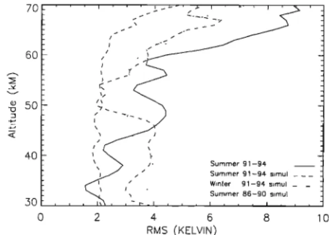
Figure 1. Standard deviations of the temperature mean dif-

ferences between measurements obtained with lidar located at

Biscarosse (CEL) and at Saint-Michel de l'Observatoire (OHP). Data obtained in summer (April-September) between 1991 and 1994 are represented with a long-dashed line when instruments have operated simultaneously and with a solid line otherwise. Simultaneous data obtained in winter (October- March) between 1991 and 1994 are represented with a dashed

and dotted line. Simultaneous data obtained in summer be-

tween 1986 and 1990 are represented with a dotted line.

caused by successive improvements performed on these instru-

ments. Additionally, the lidar data are operationally computed

by integrating over the full time of operation during the night. Profiles from the two sites are obtained during a different portion of the night due to differing local weather. Thus devi- ations between the measurements made by the two instru- ments can be expected due to quasi-systematic changes (tides), or random atmospheric variability. For some seasons, there is large stratospheric variability, thus reducing the potential to detect differences associated with instrumental changes. Data selected from April to September (Figure 1) reduce the vari- ability induced by planetary waves, by gravity waves, and in- duced-mesospheric inversions above 60 km [Hauchecorne et al., 1991; Wilson et al., 1991]. When comparing profiles from both sites representing an integration period with an overlap better than 50% of the total operating time, minimum vari- ability (2 K) is observed for data acquired between April and September (summer 91-94 simul., Figure 1). Comparing data obtained between October and March (winter 91-94 simul., Figure 1), a larger variability can be noted in the upper strato- sphere and in the upper mesosphere, due to dynamical per- turbations. Data integrated over very different nighttime hours (summer 91-94, Figure 1) also exhibit an enhanced variability, mainly in the upper stratosphere and mesosphere, where tidal effects are expected to be large. Some differences are caused by misalignment of the laser beam with the field of the collec- tor telescope, through parallax or defocusing effects [Halldor- son and Langerholc, 1978]. This affected primarily the data of the OHP system associated with the lowest altitude range. The OHP lidar is based on a bistatic configuration, while the lidar

at Biscarosse is a monostatic system. In January 1991 a major

technical improvement in the alignment system was imple- mented at OHP that permits the reduction of misalignment problems and allows for checking of their amplitudes [Keckhut et al., 1993]. Comparison of both data sets before and after this change (summer 86-90 simul. and summer 91-94 simuh, Fig-

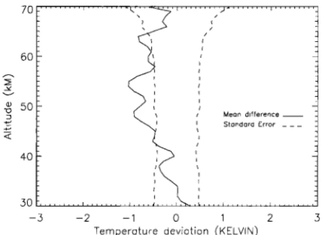
KECKHUT ET AL.: STRATOSPHERIC TEMPERATURE TRENDS 7939 70 60 • 50 40 30 x / /1 Mean difference I Standard Error -3 -2 -1 0 1 2 3

Temperoture deviotion (KELVIN)

Figure 2. Temperature mean differences (TOHP-TCEL solid line) between measurements obtained with lidar located at Biscarosse (CEL) and Saint-Michel de l'Observatoire (OHP). Estimated uncertainty based on photon-counting noise are also indicated (ill standard error is represented by dashed lines).

ure 1) reveals different mean variability. In the mesosphere the root-mean-square of the difference is reduced, due to the com- bined effects of laser power increase and decrease of sky back- ground noise. Additionally, in the lower stratosphere, one can note a reduction of the variability of the difference, attributed to the reduction of misalignment events. Finally, comparison of quasi-simultaneous summer data from April to September obtained from 1991 to 1994 (19 events) for both sites reveals a mean difference of less than 1 K (Figure 2). The difference between both data sets, obtained in a better geophysical con- figuration, have been improved, compared with the previous ones obtained. The remaining mean difference is maximum at the stratopause level (1 K) and we have not found any reason, either instrumental or geophysical, to explain it.

Temperatures measured with lidar, interpolated to a stan- dard NCEP pressure level 10 hPa, are compared with NCEP temperatures (Figure 3). Some temperature differences are observed that might be due to lidar misalignment. Then tem- perature uncertainties may be larger than expected when con- sidering that noise is not only due to the statistical noise. No systematic large positive differences are observed after January 1991 when the receiver OHP system was redesigned. Also, lidar temperatures are sometimes very cold, mainly during the 1-2 year period after the major volcanic eruptions of E1 Chi- chon and Mount Pinatubo. During other periods a systematic difference of 2 K is observed which might be due to radiosonde bias or to the residual scattering of the aerosol background. Both of these effects on lidar are expected to decrease with altitude and only the lower part of the profile need to be

removed.

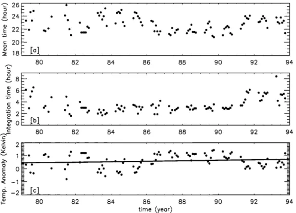
Individual lidar profiles are derived by integrating measure- ments taken during the night over several hours. The integra- tion period depends on factors such as local cloud cover, mea-

surement protocol, and availability of th• operator. In Figure 4

the monthly mean time of the middle of the period of opera- tion and the monthly mean integration time for lidar measure- ment at OHP are reported for months between April to Sep- tember. Prior to 1982, measurements were not very numerous, and the time of measurements and the integration period fluc- tuated substantially. Between 1982 and 1986, measurements

15 lO 5 0 -lO -15

Figure 3. Time evolution of the daily temperature difference between lidar and NCEP analyses (lidar - NCEP) at 10 hPa. Asterisks on the top represent major volcanic eruptions. Squares are added when OHP and CEL difference is smaller than 1 K. Vertical lines represent major instrumental changes on OHP lidar (long-dashed lines) and on NCEP analyses for lower stratospheric changes (mixed dotted and dashed lines). These last changes are mainly related to changes in data as- similation and radiosonde weight versus satellite.

were mostly centered around 2330 UT and integrated over 2-3 hours. Then up to 1991, measurements started earlier. After 1991, measurements were again centered around 2330 UT but with a significant increase of the integration time. These changes in measurement time should have induced residual temperature changes due to tidal fluctuations. In the summer, stratospheric temperature tides contain a diurnal cycle with an amplitude around the stratopause of 4 K (from minimum to maximum) peaking at 1800 solar local time [Keckhut et al., 1996]. Temperature anomalies have been estimated according to these tidal characteristics and the exact period of the lidar sounding at OHP (Figure 4). The simulation shows tidal effects associated with interannual changes smaller than 1 K, with

most of the structure between 1986 and 1991. Because of the

length of the integration time, to the operations restricted to nighttime, and mainly centered around the beginning of the night, the tidal induced effect on lidar should not be the largest except in the case of a systematic change of the time of mea- surement between the beginning and the end of the series. The overall residual, nonatmospheric trend for this period is smaller than +0.2 K per decade.

3. NCEP Temperature Analyses

Temporal continuity in the NCEP analyses has been inves- tigated by different methods: comparison with rockets, step regression analyses, and comparison of data for adjacent peri- ods, with slightly different results [Gelman et al., 1986]. Differ- ences among these methods of 2-4 K are obtained, giving an estimation of the magnitude of adjustment uncertainties. Ad- justments were derived by systematic comparisons with rocket measurements from several sites, mostly over the North Amer- ican continent. Rayleigh lidar operating in the south of France during the same periods were compared with the interpolated adjusted NCEP data. Differences of few Kelvins were reported [Chanin and Gelman, 1989]. Abrupt changes appear coincident with dates of satellite replacements, mainly at 2 and 1 hPa levels (Figure 5). Large differences were also reported when

7940 KECKHUT ET AL.: STRATaSPHERIC TEMPERATURE TRENDS 24-

I I

[ø]

E 6•

> 2

=

...

•

,.

.' -,

..'. :., .,- ...

ß

.

E 0

ß ß

.;

'"

.'"

ß

Figure 4. (a) Time evolution of the monthly mean time of lidar measurement, (b) the integration time and (c) the anomalies induced by tides in assuming a diurnal cycle with an amplitude of +_2 K and a maximum

around 1800 LST.

NCEP analyses were compared with some single site rocket

data [Finger et al., 1993]. Some of these are due to satellite

timing issues.

NCEP global strataspheric temperature maps are generated from analyses [Cressman, 1959] of TOVS data measured from

0600 to 1800 UT. The time which should be attributed at a

particular location for each day in the NCEP analyses is com-

plex. The NCEP strataspheric analyses are derived from one of

15

o

Figure 5. Time evolution of the daily temperature difference between lidar and NCEP analyses (lidar - NCEP) at i hPa. Vertical dashed lines represent changes on satellite or failures on TOVS. Horizontal bars located on the top and bottom indicate, respectively, morning and afternoon orbits over Eu-

rope. Periods between two satellite changes are labelled (see

text and Finger et al. [1993]).

two operational, polar orbiting, Sun-synchronous satellites. One satellite has its ascending equatorial crossing near 1330 LT (afternoon satellite) and the other its descending crossing near 0730 LT (morning satellite). The time of data at a geo- graphic location may change drastically when data used in the analysis change from the morning to the afternoon satellite. Prior to 1985 the SSU was included on morning and afternoon satellites, but after 1985, SSU instruments were on only after- noon satellites. An additional complication occurs in recent years, when SSU is on only the afternoon satellite. In that case,

the time on the data is that associated with the satellite used for the lower-level information. This was an issue when the

primary satellite was NOAA 10, which had no SSU. NOAA 10

data (with no SSU) used SSU data from NOAA 9 for upper

strataspheric information. The SSU data came from the latest

pass of the secondary satellite (NOAA 9 or NOAA 11). How-

ever, the time on the data was from NOAA 10, even though the

NOAA 9 information was not within 1200 ___ 0600 UT. Over

much of the United States the analysis used the descending orbit for all periods (see Finger et al. [1993] and Figure 5 for period definitions). Over France the analysis used ascending data (near 1400 to 1500 LT) for periods 2, 5, 7, 8, and 11;

during periods 3, 4, and 6, descending data (near 0800 LT);

and for periods 9 and 10, descending data near 0130-0330 LT. It is the switch, from Europe and the United States, using the same orbit, to Europe and the United States using different orbits, which causes problems (see formula 5 in Appendix A).

Lidar temperatures are systematically higher than NCEP

values when satellite measurements were obtained around 0800 UT over OHP and lower when satellite measurements were obtained around 1400 UT over OHP. Data from several

KECKHUT ET AL.: STRATOSPHERIC TEMPERATURE TRENDS 7941

lidars located at different sites were statistically compared with the corresponding NCEP data [WiM et al., 1995], revealing a large dispersion of the individual mean differences. This dis- persion proved to be due mostly to tidal effects. A time-of-day adjustment using Microwave Limb Sounder data (from the Upper Atmospheric Research Satellite) reduced the disper- sion. The comparison of the lidar data with the NCEP data at OHP reveals an alternating feature, which seems to be corre-

lated more with the time of the measurements (Figure 5) than

with the satellite used. This effect appears from 2 hPa to 0.4 hPa but is more obvious at 1 hPa. These results seem to suggest a further tidal effect in the adjustment data. Over many years, changes of satellite orbits induced sudden changes of the local

time of the measurements. Twelve rocket sites from 8øS to

77øN were originally used for adjustments [Finger et al., 1993]. However, after 1980, severe curtailing of the number of launches occurred; also, two high-latitude sites stopped oper- ating, reducing the rocket network. Adjustments, based on rockets launched from U.S. sites mostly around 0800-1000 LT, do not differentiate temperature changes of instrumental ori- gin versus deviations induced by the portion of the diurnal cycle observed (formula 1 in Appendix A). NCEP data over rocket sites, mostly located over the United States, present systematic time differences due to tidal effects in the satellite data. Temperature adjustments obtained in the NCEP-rocket data comparisons correspond to both instrumental bias and to differential tidal effects (formula 2 in Appendix A). NCEP- adjusted temperatures over the United States are not affected by either instrumental bias or satellite orbit changes because both effects are mixed together and adjusted by comparison

with rockets. The mean time of measurement for the rocket

network did not change, so the NCEP continuity over the United States was insured (formula 3 in Appendix A).

However, when adjustments are applied on NCEP maps over some places corresponding to the opposite orbit phase from the United States (such as Europe), instrumental biases are removed, but a more complex bias remains (formula 5 in Appendix A). This will have no consequence on the temporal continuity of the data series if timing of satellite orbits does not switch. However, satellite orbits do switch several times every 2-3 years, providing shifts of the local time of the TOVS measurements over a single location. Thus abrupt changes may appear for each switch of the orbit of the satellite. If the

instrumental bias between two successive satellite instruments

may be removed using this procedure, some abrupt tempera- ture changes are likely over Europe due to the residual tidal effects (formula 6 in Appendix A). For NCEP maps the time of measurements oscillates between morning and afternoon local time depending on the orbit phase considered. In the upper stratosphere, tidal changes are dominated by a diurnal oscilla- tion, with an amplitude of 2 to 3 K, reaching a maximum around 1800 LT [Keckhut et al., 1996]. The expected range of differences of 4-6 K appears to be in good agreement with observed mean differences (over periods having the same sat- ellite orbit) between lidar and interpolated NCEP analyses. For the last satellite transition reported here (1991), the tem- perature drift is less obvious; however, one has to notice that the number of rocket profiles drastically decreased, and time of launches were more random. Also, some bias in the sampling of the diurnal cycle related to an eastward drift of some sat- ellites or orbital decay effects has already been reported [Wentz and Schabel, 1998; Christy et al., 1999]. This implies that some and (mainly the last) adjustments may be less accurate and

break slightly the adjustment procedure and systematic bias. Additionally, though periods 9 and 10 were measured over France in the morning, they were very early morning (0130- 0320 LT), not midmorning (0730 LT), as for periods 3, 4, and

6. These characteristics lead to reduced tidal effects. The time

of day effect was reported [Pick and Brownscombe, 1981; Nash and Forrester, 1986] when SSU radiances obtained simulta- neously on two distinct satellites were compared. A certain similarity in the anomalies between the 1 hPa and the 10 hPa levels can be noted. However, amplitude of tides are expected to be around 3 times smaller and cannot be explained accord- ing to the knowledge of the error sources either on lidar or on NCEP analyses.

4. Comparison of the Long-Term Changes

To overcome instrumental effects, data have been filtered. A

lidar subset has been produced which should be free of distur- bances caused by volcanic aerosols or misalignment events.

When the difference between NCEP and lidar at 10 hPa is

larger than I K, we may suspect a misalignment problem, and so the lower part of the temperature profile is removed up to a certain level where we have supposed the alignment problem negligible. This is based on some approximate functions of the misalignment with altitude [Keckhut et al., 1993], which shows that the disturbance is sharply decreasing with altitude follow- ing a square function of the altitude. Lidar profiles contami- nated by volcanic particles such as after E1 Chich6n (April

1982) and Pinatubo (June 1991) eruptions, were limited to

altitudes above 40 km to the top. Dates of lidar misalignment were found from the comparison with NCEP temperatures at

10 hPa. A difference of 2 K is systematically observed with lidar when no geometric obstruction or high volcanic pollution are expected, as reported previously for periods after June 1991, or when CEL and OHP are in good agreement. Standard aerosol measurements with one wavelength and a radiosonde as an air density reference (as performed at OHP) cannot permit to detect with a high degree of confidence a scattering ratio

smaller than 1.05. Even with a Raman channel, the uncertain-

ties of aerosol lidar measurements remain larger than several percent. With such an error the associated temperature bias can be as large as 10 K. The approach proposed here, to

eliminate the effect of such events, is to use the 10 hPa NCEP

analyses as a reference and to estimate the potential distur- bances on each individual lidar profiles with altitude. The low- est valid altitude is decided when the estimated anomaly is expected to become smaller than 1 K. According to this test,

some data have been removed below this altitude on each

corresponding lidar profile.

The operational NCEP maps include discontinuities be- tween places where adjustments are derived (mostly from

rocket data over the United States) and places (such as Eu-

rope) where an opposite orbit phase may exist. Because of data averaging, discontinuities in the zonal means should be smaller than discontinuities in the data interpolated to a site. Thus it may be informative to include zonal mean data in a compari- son of trend estimates. The same linear regression analysis already applied on lidar and rocket measurements [Hau- checorne et al., 1991; Keckhut et al., 1995, 1998] is applied on the three data sets. Lidar data are interpolated to a given pressure level using NCEP geopotential heights. The trend analysis is based on a least squares fit of the weekly mean series by a linear combination of proxy functions, including seasonal,

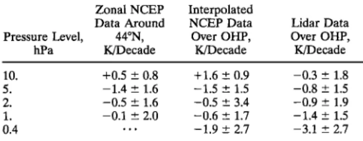
7942 KECKHUT ET AL.: STRATOSPHERIC TEMPERATURE TRENDS Table 1. Trend Coefficients for Levels Between 10 and 0.4

hPa Using NCEP Analyses (Zonal Mean and Data Interpolated Over OHP) and OHP Lidar Data a

Zonal NCEP Interpolated

Data Around NCEP Data Lidar Data Pressure Level, 44øN, Over OHP, Over OHP,

hPa K/Decade K/Decade K/Decade 10. +0.5 +_ 0.8 +1.6 + 0.9 -0.3 +_ 1.8 5. -1.4 +_ 1.6 -1.5 + 1.5 -0.8 _+ 1.5 2. -0.5 +_ 1.6 -0.5 + 3.4 -0.9 +_ 1.9 1. -0.1 +_ 2.0 -0.6 +_ 1.7 -1.4 +_ 1.5 0.4 .... 1.9 + 2.7 -3.1 _+ 2.7

a95% confidence intervals are also indicated.

solar, quasi-biennial oscillation (QBO), and trend components. No stratospheric aerosol forcing is included because no effect in the summer upper stratosphere is expected at midlatitude [Rind et al., 1992] nor observed [Keckhut et al., 1995]. Only "summer" months (April to September) are used, presenting the lowest atmospheric variability for these latitudes [Hau- checorne et al., 1991; Leblanc et al., 1998]. Confidence limits are estimated by taking account of the autocorrelation coefficients between successive data. The results are compiled in Table 1.

At 10 hPa, trends deduced from filtered lidar data are smaller

than with the full data set by a factor of nearly 10 and are in better agreement with theoretical estimates. This invalidated previous trend results [Keckhut et al., 1996] with OHP lidar below 35 km, as suspected. However, as shown by the statistical

confidence bars, this trend estimate is uncertain due to the

severe filtering we have done on the data to remove misalign- ment effects. The NCEP zonal mean analysis reveals a trend in a reasonably good agreement with lidar. Some radiosonde temperature series suffer bias and temporal inhomogeneities mostly in the stratosphere [Gaffen, 1994; Zhai and Eskridge, 1996; Parker et al., 1997]. The difference between zonal and interpolated NCEP temperatures may suggest some disconti-

nuities due to the radiosonde over the south of France in-

cluded in NCEP analyses. Estimated trends at this level may also differ due to changes in the NCEP analyses. At 5 hPa, interpolated and zonal NCEP mean data give similar trends

but twice the one observed with the filtered lidar series. At 1

hPa, lidar data give a nearly significant result. The interpolated and zonal NCEP data set presents smaller trends. At 2 hPa, similar abrupt changes are observed in NCEP-lidar compari- sons with smaller amplitudes, and the trend observed with lidar is still twice the one observed with NCEP temperatures. At 0.4 hPa, where the largest cooling trend is observed with lidar, a smaller one is reported by NCEP analyses. At this level, NCEP is known to be quite noisy.

5. Discussions and Prospects

Rockets, which provided the basis for the NCEP adjustment system, are no longer available in quantity. To continue to ensure long-term consistency, lidars operating within the framework of the Network for Detection of Stratospheric Change can replace rocket soundings. However, the present study reveals that some biases have existed in lidar tempera- ture profiles, mostly around the lower part of the profiles. Comparisons between lidar and interpolated NCEP tempera- tures at 10 hPa allow the detection of periods of large mis- alignment or stratospheric aerosol loading. However, interpo-

lated NCEP temperatures at 10 hPa use radiosonde data, which also may have instrumental discontinuities. Some spe-

cific technical solutions exist to resolve these lidar limitations.

At OHP this problem has been solved by using a specific configuration with a large field of view for the low-sensitivity channel independent of the main channel having a small field

of view. Recent data have shown that this solution is efficient.

Also, lidar alignment will be operationally improved through an automatic procedure driven by a computer that will guar- antee its repeatability. For the aerosol limitation, the temper- ature profile can be extended downward with Raman channels [Keckhut et al., 1990; Hauchecorne et al., 1992]. For the period during which the Raman channel was not available, a very sensitive method for detecting the top of the aerosol layer with one wavelength using the variance of the signal [Hauchecorne et al., 1994], may be applied on past data. Similarly, other lidars have been developed under the framework of the Network of Detection of Stratospheric Change [Kurylo and Solomon, 1990]. These lidar stations are located in various regions from 80øN to 78øS, providing the ability to evaluate NCEP adjust- ments as a function of latitude. Tropical stations Hawaii (19.5øN) and La R•union (21øS) are valuable because variabil- ity is small year-round at these latitudes [Leblanc et al., 1998]. Though there is little coverage in longitude in the tropics, in the northern midlatitudes, OHP (44øN) and Table Mountain Facility (34øN) provide very different longitudes, which can help to take into account tidal effects. Maintaining a stable lidar measurement time is very important. For the OHP lidar we plan a reprocessing of the entire database by selecting

measurements over the same time window. An observation

time histogram reveals that during most nights, measurements exist between 2100 and 2300 UT. This filtering procedure will only slightly reduce the number of profiles and should decrease

the tidal effects.

Upper stratospheric NCEP database adjusted with U.S.- based rockets may lead to adequate adjustments for data in- terpolated over the midlatitude United States (see Appendix A), allowing for an accurate trend estimate for this region. However, series above 2 hPa (where tides exhibit large ampli- tudes), interpolated over other regions and zonal means, are biased and trends flawed. The main problem of the current NCEP adjustment procedure is that tidal effects and instru- ment adjustments are combined.

A solution is to produce two separate maps, one containing ascending data and the other descending data, with two sepa- rate local times from each for the entire globe. When new satellites are introduced and timing changes occur, these can be well documented. Both maps can be combined to create a 24 hour ascending plus descending map as needed. Current plans are that NCEP will continue the current 1200 UT to insure continuity with the traditional product and, additionally, to produce the separate ascending and descending maps.

For remaining tidal effects, a time of day correction can be used. A simple statistical model to consider tidal effects does not seem to be an adequate solution (tested by Keckhut et al. [1996]) probably due to the large variability of tides. Moreover, tide amplitudes may be modified both on a daily and on a long-term basis along with ozone, water vapor, and tempera- ture field changes. Tidal change associated with the expected global stratospheric cooling and ozone changes needs to be simulated and quantified. This kind of study was done for the surface level [Hansen et al., 1995] and should be conducted also for the stratosphere where ozone forcing leads to a clear sys-

KECKHUT ET AL.: STRATOSPHERIC TEMPERATURE TRENDS 7943 tematic tidal effect of several Kelvin. Real-time tidal monitor-

ing might be required. Lidar operating continuously during the night may be used to quantify tidal effects [Gille et al., 1991; Dao et al., 1995; Leblanc et al., 1999]. However, such a possi- bility is restricted mainly to winter when the fraction of the night is sufficient to separate 12 and 24 hour components. During summer, tidal observations with lidar are not possible until daytime measurements are improved and implemented as routine measurements. Depending on the tide sensitivity to global atmospheric changes, one can use a climatic tidal model or continuous tidal monitoring. These results will be helpful for any satellite adjustments and stratospheric temperature data comparisons not performed at the same local time.

Appendix A

NCEP adjustments (Adj) as applied to produce actual NCEP stratospheric temperature [Gelman et al., 1986] can be expressed by this simplified formula:

Adj- rTovs- rRo C = lB + drtide(tx)- drtide(tROC) (A1)

with TTovs and TRO½, respectively, the raw temperature mea- sured by TOVS and by rockets over the United States, d Ttide the temperature anomaly induced by tides for a given solar local time tRo½, tx, respectively, the time of measurement for

rockets and for both orbit phases (ascending and descending) of TOVS included in the _+6 hours window, and IB the instru-

mental bias between two successive radiometers.

The NCEP adjusted temperature TNCEP is given by

6. Summary and Conclusions

Lidar data and NCEP data have been compared for the OHP site from 1979 to 1993. A temperature series obtained from an independent nearby lidar station have been also com- pared with the OHP lidar database. Some of the differences can be explained by either an instrumental bias in the OHP lidar system (as the presence of volcanic aerosols injected in the stratosphere or misalignment effects) or tidal effects in the upper stratospheric NCEP data. Lidar instrumental problems

have been identified, but these effects cannot be corrected a

posteriori, so past lidar data must be filtered. Biases of 2 to 5 K, morning versus afternoon orbit effect, have been suggested through NCEP-lidar comparisons. Adjustment procedure have been described in Appendix A, and tidal changes appear to be the possible source of such discrepancy. In addition to instru- mental bias, which has been the highlight in these studies, temperature trends have been estimated, taking advantage of NCEP-lidar comparisons and instrumental limitations. Trends were found to be between few tenths of a degree per decade around 30 km and few degrees per decade at the stratopause level. Despite the fact that trend confidence is already poor, observed trends are in a relatively good agreement with radi- ative transfer models [Miller et al., 1995] which expect a cooling

of 0.4 K/decade around 30 km to 1.1 K/decade at 45 km,

because of CO2 increase and ozone decrease.

Successive improvements on the OHP lidar systems have already reduced instrumental bias in the lower part of the profile for current measurements. Further improvements, such as automatic alignment, Raman channels, and detection of aerosols by tests on signal variance, have been planned for routine operations and should improve lidar data quality and the temporal continuity in the future. In the future, it is pro- posed to separate ascending and descending TOVS data to insure instrument adjustments and then combine both maps to produce 24 hour NCEP analyses.

Because of the local nature of lidar, only satellite data are expected to provide global trend estimates and the detection of regional patterns. However, comparisons between the lidar and the NCEP temperature records show that the successive morning and afternoon satellites include tidal temperature dif- ferences. Atmospheric tides and the successive switches of orbits must be addressed in any adjustment procedure. Theo- retical estimates of such effects are in good agreement with the data comparisons.

TNCEP '-- TTOVS(tx)- mdj = rtrue q-drtide(tx) q- IB- mdj (m2)

with Ttrue the right measured temperature.

For the TOVS data obtained at the same orbit phase than the one used for TOVS/rocket comparisons, using (A1) and (A2), one obtains a temperature TNCEP independent to orbit

shifts

TNCEP-- rtru e q- dTtide(tROC ). (A3) However, for the other orbit phase, NCEP-adjusted temper- ature TNCEP is given by the following formulas, including tidal

effect associated with orbit shifts,

TNCEP -- rtrue q- drtide(ta) -- drtide(td) q- drtide(tROC) (A4a) TNCEP = rtrue q- drtide(td) -- drtide(ta) q- drtide(tROC) , (A4b)

with t,, td, respectively, the time of measurement for the ascending and descending orbit phases of TOVS.

Note from (A3) and (A4) that the 1200 UT-adjusted NCEP temperature maps include inhomogenous temperature biases according to both possible orbit phases.

Also, if the orbit phase is reversed with time, then for places where TOVS has observed with the same orbit phase than the United States (used for comparison with rockets) and accord- ing to (A3), no tidal biases are observed. On the contrary, for places (having the opposite orbit phase) such as Europe, a

sudden temperature change Tdiscontinuity exists with an ex-

pected amplitude deduced from (A4a) and (A4b) as follows:

Tdiscontinuity

-- 2[Drtide(ta)

-- Dttide(td)

].

Acknowledgments. Some preliminary studies on this topic were

performed while Philippe Keckhut held a National Research Council/ NOAA Research Associateship. The authors would like to acknowl-

edge all the lidar operators at CEL (Bain, Bourdary, and Martinez) and at OHP (Gabelou, Schneider, Syda, and Velghe).

References

Brasseur, G., M. H. Hitchman, S. Walter, M. Dymek, E. Falise, and M.

Pirre, An interactive chemical dynamical radiative two-dimensional model of the middle atmosphere, J. Geophys. Res., 95, 5639-5655,

1990.

Chanin, M. L., and M. E. Gelman, Comparison between stratospheric

temperature from NMC analyses and lidar data, Proc. IRS, 88,

7944 KECKHUT ET AL.: STRATOSPHERIC TEMPERATURE TRENDS

Christy, J. R., R. W. Spencer, and W. D. Braswell, Global temperature

variations since 1979, paper presented at the 10th Symposium on Global Change Studies, Am. Meteorol. Soc., Dallas, Tex., January 10-15, 1999.

Cressman, G. P., An operational objective analysis system, Mon. Weather Rev., 87, 367-374, 1959.

Dao, P. D., R. Farley, X. Tao, and C. S. Gardner, Lidar observations of the temperature profile between 25 and 103 km: Evidence of strong tidal perturbation, Geophys. Res. Lett., 22, 2825-2828, 1995.

Finger, F. G., M. E. Gelman, J. D. Wild, M. L. Chanin, A. Hau-

checorne, and A. J. Miller, Evaluation of NMC upper stratospheric

temperature analyses using rocketsonde and lidar data, Bull. Am.

Meteorol. Soc., 74, 789-799, 1993.

Gaffen, D. J., Temporal inhomogeneities in radiosonde temperature records, J. Geophys. Res., 99, 3667-3676, 1994.

Gelman, M. E., and R. M. Nagatani, Objective analyses of height and

temperature at the 5-, 2-, and 0.4 mb levels using meteorological rocketsonde and satellite radiation data, Adv. Space Res., XVII,

117-122, 1977.

Gelman, M. E., A. J. Miller, K. W. Johnson, and R. M. Nagatani,

Detection of long-term trends in global stratospheric temperature from NMC analysis derived from NOAA satellite data, Adv. Space

Res., 6, 17-26, 1986.

Gille, S. T., A. Hauchecorne, and M. L. Chanin, Semidiurnal and diurnal tidal effects in the middle atmosphere as seen by Rayleigh lidar, J. Geophys. Res., 96, 7579-7587, 1991.

Guirlet, M., P. Keckhut, S. Godin, and G. Megie, Study of the long- term evolution of the stratospheric ozone vertical distribution at

Observatoire de Haute-Provence (43.9øN, 5.7øE) using different in- strumental techniques, Ann. Geophys., in press, 2000.

Halldorson, T., and J. Langerholc, Geometrical form factors for the lidar function, Appl. Opt., 17, 240-244, 1978.

Hansen, J., M. Sato, and R. Ruedy, Long-term changes of the diurnal temperature cycle: Implications about mechanisms of global climate change, Atmos. Res., 37, 175-209, 1995.

Hauchecorne, A., M. L. Chanin, and P. Keckhut, Climatology of the middle atmospheric temperature (30-90 km) and trends as seen by Rayleigh lidar above south of France, J. Geophys. Res., 96, 15,297-

15,305, 1991.

Hauchecorne, A., M. L. Chanin, P. Keckhut, and D. Nedeljkovic, Lidar

monitoring of the temperature in the middle and lower atmosphere, Appl. Phys., Set. B, 55, 29-34, 1992.

Hauchecorne, A., P. Keckhut, and C. Souprayen, The notion of vari-

ance in the data analysis of Rayleigh-Mie lidar signal, paper pre-

sented at the 17th International Laser Radar Conference, NASA, Sendai, July 25-29, 1994.

Hood, L. L., J. L. Jirikowic, and J.P. McCormack, Quasi-decadal variability of the stratosphere: Influence of long-term solar ultravi- olet variations, J. Atmos. Sci., 50, 3941-3958, 1993.

Karl, T. R., R. Q. Quayle, and P. Y. Groisman, Detecting climate variations and change: New challenges for observing and data man-

agement systems, J. Clim., 6, 1481-1494, 1993.

Keckhut, P., M. L. Chanin, and A. Hauchecorne, Stratosphere tem- perature measurement using Raman lidar, Appl. Opt., 29, 5182- 5186, 1990.

Keckhut, P., A. Hauchecorne, and M. L. Chanin, A critical review of the database acquired for the long term surveillance of the middle

atmosphere by the French Raleigh lidar, J. Atmos. Oceanic Technol.,

10, 850-867, 1993.

Keckhut, P., A. Hauchecorne, and M. L. Chanin, Midlatitude long- term variability of the middle atmosphere: Trends, cyclic, and epi- sodic changes, J. Geophys. Res., 100, 18,887-18,897, 1995.

Keckhut, P., et al., Semidiurnal and diurnal temperature tides (30-55 km): Climatology and effect on UARS-lidar data comparisons, J.

Geophys. Res., 101, 10,299-10,310, 1996.

Keckhut, P., F. J. Schmidlin, A. Hauchecorne, and M. L. Chanin,

Trend estimates from US rocketsondes at low latitude stations (8 S-34 N), taking into account instrumental changes and natural vari- ability, J. Atmos. Sol. Terr. Phys., 51,447-459, 1998.

Kurylo, M. J., and S. Solomon, Network for the Detection of Strato- spheric Change, NASA Rep., Code EEU, 1990.

Lambeth, J. D., and L. B. Callis, Temperature variations in the middle

and upper stratosphere: 1979-1992, J. Geophys. Res., 99, 20,701, 1994.

Leblanc, T., I. S. McDermid, P. Keckhut, A. Hauchecorne, C. Y. She, and D. A. Krueger, Temperature climatology of the middle atmo- sphere from long-term lidar measurements at middle and low lati-

tudes, J. Geophys. Res., 103, 17,191-17,204, 1998.

Leblanc, T., I. S. McDermid, and D. A. Ortland, Lidar observation of the middle atmospheric tides, Comparison with HRDI and GSWM,

part I, Methodology and winter observations over Table Mountain (34.4 N), J. Geophys. Res., 104, 11,917-11,929, 1999.

Miller, A. J., R. M. Nagatini, G. C. Tiao, X. F. Niu, G. C. Reinsel, D.

Wuebbles, and K. Grant, Comparisons of observed ozone and tem-

perature trends in the lower stratosphere, Geophys. Res. Lett., 19, 929-932, 1992.

Miller, A. J., G. C. Tiao, C. Reinsel, D. Wuebbles, L. Bishop, J. Kerr, R. M. Nagatini, J. J. DeLuisi, and C. L. Mateer, Comparisons of

observed ozone trends in the stratosphere through examination of

Umkehr and balloon ozonesonde data, J. Geophys. Res., 100,

11,209-11,217, 1995.

Nash, J., and G. F. Forrester, Long-term monitoring of stratospheric

temperature trends using radiance measurements obtained by the TIROS-N series of NOAA spacecraft, Adv. Space Res., 6, 37-44, 1986.

Parker, D. E., M. Gordon, D. M. H. Sexton, C. K. Folland, and N.

Rayher, A new global gridded radiosonde temperature database and

recent temperature trends, Geophys. Res. Lett., 24, 1499-1502, 1997.

Pick, D. R., and J. L. Browscombe, Early results based on the strato- spheric channels of TOVS on the TIROS-N series of operational

satellites, Adv. Space Res., 1, 247-260, 1981.

Randel, W. J., and J. B. Cobb, Coherent variations of monthly mean

total ozone and lower stratospheric temperature, J. Geophys. Res.,

99, 5433-5447, 1994.

Rind, D., R. Suozzo, N. K. Balanchandra, and M. J. Prather, Climate

change and the middle atmosphere, I, The doubled CO2 climate, J.

Atmos. Sci., 47, 475-494, 1990.

Rind, D., R. Suozzo, N. K. Balachandra, and M. J. Prather, Climate

change and the middle atmosphere, part II, The impact of volcanic

aerosols, J. Clim., 5, 189-207, 1992.

Smith, W. L., H. M. Woolf, C. Hayden, D. Q. Wark, and L. M. McMillin, The TIROS-N operational vertical sounder, Bull. Am. Meteorol. Soc., 60, 1177-1187, 1979.

Stratospheric Processes and Their Role in Climate/International

Ozone Commission/Global Atmospheric Watch (SPARC/IOC/ GAW), Assessment of trend in the vertical distribution of ozone,

SPARC Rep. 1, WMO Rep. 43, edited by N. Harris, R. Hudson, and

C. Phillips, World Meteorol. Organ., Geneva, Switzerland, 1998. Swinbank, R., et al., Stratospheric tides and data assimilation, J. Geo-

phys. Res., 104, 16,929-16,941, 1999.

Wentz, F. J., and M. Schabel, Effects of orbital decay on satellite- derived lower-tropospheric temperature trends, Nature, 394, 661- 664, 1998.

Wild, J. D., et al., Comparison of stratospheric temperature from

several lidars using NMC and MLS data as transfer reference, J. Geophys. Res., 100, 11,105-11,111, 1995.

Wilson, R., M. L. Chanin, and A. Hauchecorne, Gravity waves in the

middle atmosphere by Rayleigh lidar, part 2, Climatology, J. Geo-

phys. Res., 96, 5169-5183, 1991.

World Meteorological Organization, Scientific assessment of strato-

spheric ozone: 1989, WMO Rep. 20, Global Ozone Res. and Monit.

Proj., Geneva, Switzerland, 1989.

Zhai, P., and R. E. Eskridge, Analyses of inhomogeneities in radio- sonde temperature and humidity time series, J. Clim., 9, 884-894, 1996.

A. Hauchecorne and P. Keckhut, Service d'A•ronomie/IPSL, BP3,

91371 Verri•res-le-Buisson, France. ([email protected]) J. D. Wild, Research and Data Systems Corporation, Greenbelt,

MD 20770.

M. Gelman and A. J. Miller, Climate Prediction Center, NCEP/ NOAA, Washington, DC 20203.

(Received January 28, 2000; revised November 20, 2000; accepted November 22, 2000.)