A new era in hydrofluoric acid solution calorimetry: Reduction of required sample size below ten milligrams.

HAL Id: hal-00077571

https://hal-insu.archives-ouvertes.fr/hal-00077571

Submitted on 31 May 2006

HAL is a multi-disciplinary open access

archive for the deposit and dissemination of

sci-entific research documents, whether they are

pub-lished or not. The documents may come from

teaching and research institutions in France or

abroad, or from public or private research centers.

L’archive ouverte pluridisciplinaire HAL, est

destinée au dépôt et à la diffusion de documents

scientifiques de niveau recherche, publiés ou non,

émanant des établissements d’enseignement et de

recherche français ou étrangers, des laboratoires

publics ou privés.

A new era in hydrofluoric acid solution calorimetry:

Reduction of required sample size below ten milligrams.

Guy L. Hovis, Jacques Roux, Pascal Richet

To cite this version:

Guy L. Hovis, Jacques Roux, Pascal Richet. A new era in hydrofluoric acid solution calorimetry:

Reduction of required sample size below ten milligrams.. American Mineralogist, Mineralogical Society

of America, 1998, 83, pp.931-934. �hal-00077571�

931 0003–004X/98/0708–0931$05.00

A new era in hydrofluoric acid solution calorimetry: Reduction of

required sample size below ten milligrams

G

L. H

,

* J

R

,

P

R

1_{Department of Geology and Environmental Geosciences, Lafayette College, Easton, Pennsylvania 18042, U.S.A.} 2_{CNRS-CRSCM, 1A, rue de la Ferollerie, 45071 Orleans Cedex 2, France}

3_{Institut de Physique du Globe, 4, place Jussieu, 75005 Paris, France}

A

Significant advances have been made in hydrofluoric acid solution calorimetry at La-fayette College in the past 15 years. To determine the degree to which these developments enable the reduction of sample size, calorimetric experiments were performed on hexagonal germanium oxide as a function of sample weight. The resulting calorimetric data indicate that the highest degrees of reproducibility (₆0.1%) are maintained down to sample sizes of 50 mg, and that precisions of 61%, acceptable for many applications, are observed to sample sizes of 10 mg. Because silicate systems produce weight-based heats of solution that are about twice that of germanium oxide, the required sample size for these will be even less. The new minimum required sample size of 5 to 25 mg (depending on applica-tion) is about two orders of magnitude less than that used 20 or 30 years ago. This makes possible many new kinds of projects for HF solution calorimetric investigation, including those on high-pressure materials.

I

Hydrofluoric acid (HF) solution calorimetry (see Wald-baum and Robie 1971 or Robie and Hemingway 1972) has long had the reputation of requiring large sample sizes. Indeed, 20 to 30 years ago it was commonplace in such work to use sample sizes of 750 to 1000 mg per dissolution (e.g., Waldbaum and Robie 1971 or Hovis 1974). More than a decade ago, however, the emerging availability of various kinds of electronic apparatus proved calorimetric measurements. More recently, im-proved digital voltmeters have further increased the pre-cision with which (typically low) calorimetric voltages can be measured. Although smaller sample sizes have been employed for years on the Lafayette College calori-metric system as a result of these enhancements, it is only recently that we have tested our system in terms of how these improvements relate to new limits on sample size.

HF

In principle a hydrofluoric acid solution calorimetric experiment is simple. One dissolves a substance in HF (our experiments normally use a 20.1 wt% solution) and measures the temperature change that ensues. Then, by measuring the heat capacity (given as energy/degree) of the dissolution vessel (calorimeter), one associates the ob-served temperature change with a corresponding energy change. Knowing the weight of the sample dissolved, one

* E-mail: hovisguy@lafvax.lafayette.edu

converts this energy into energy per gram or energy per mole: Voila, the heat (or enthalpy) of solution.

What makes high-precision calorimetry difficult is that the temperature changes (_DT) associated with dissolution

and with the determination of calorimetric heat capacity (accomplished by heating the calorimeter electrically and measuring the resulting temperature change) are normally very small, so they must be measured with extreme pre-cision. The smaller the sample, the smaller is the DT of

dissolution. Moreover, it is impossible to isolate the cal-orimeter well enough to completely eliminate the ex-change of heat with its environment, so one must be able to rigorously correct the observed values ofDT for such

exchange; this too requires highly precise temperature de-terminations. Finally, even the best calorimetric measure-ments are of little value if sample weight is not known with a high degree of accuracy.

To minimize the energy exchanged between the calo-rimeter and its environment, before the start of an exper-iment, the calorimeter and its contents are heated to a temperature close to (but just below) that at which dis-solution is to occur (in our case, normally 508C). More-over, the calorimeter is submerged in a medium (for our system a water bath) whose temperature is held constant near the intended dissolution temperature. (Note that there is a distinction between the bath temperature, Tbath,

and the convergence temperature of the system, Tconvergence,

the temperature to which the calorimeter would drift at infinite time; the small difference between the two is due to the addition of heat to the calorimeter from stirring.) In addition, the calorimeter is physically isolated from the

932 HOVIS ET AL.: HF SOLUTION CALORIMETRY USING SMALL SAMPLES

FIGURE1. The scanned plot of

tem-perature against time for an actual calor-imetric experiment employing current equipment and data reduction techniques. Lines are least-squares fits to densely packed data points that collectively are not discernible from the lines themselves. Note that the drift period at the beginning of the experiment has a positive slope, while that at the end is negative, as ex-plained in the text. The jump in temper-ature at the beginning of a heating period is associated with superheating of the thermometer, just as the precipitous de-crease in temperature at the end of a heat-ing period is related to subsequent ther-mal equilibration after the heater is turned off; these are accounted for in the data reduction. The overall temperature increase during most experiments, in-cluding temperature rises during heating periods, is on the order of 1 8C. The 0.0628CDT of dissolution in this

exper-iment is about 20 times those of the 10 mg samples in Table 1.

bath inside a stainless steel container (called a ‘‘subma-rine’’), and a moderately high vacuum (1025 _{torr) is}

es-tablished between the inner submarine and outer calorim-eter walls. Because calorimetric temperatures generally rise during an experiment, the calorimeter gains heat from its environment at the beginning of an experiment (Tcalorimeter,Tconvergence), but loses heat by the conclusion of

an experiment (Tcalorimeter.Tconvergence).

I

HF

A temperature-time plot of a typical calorimetric ex-periment, utilizing current apparatus, is shown in Figure 1. During such an experiment there are four so-called drift periods, one on each side of a heating or dissolution period. Drift periods, normally 50 min long, are periods when calorimetric temperature is monitored as a function of time while no other processes are occurring. They re-flect the rate of heat exchange between the calorimeter and its environment, but more importantly they allow cor-rection to the observed values of _DT for heat exchange

that occurs during heating (calibration) and dissolution periods. Because the calorimeter and bath temperatures are close to one another at all times, heat gained or lost by the calorimeter is generally small. Moreover, the pres-ence of the vacuum results in changes of temperature dur-ing drift periods that are for all practical purposes linear (nonlinearity being undetectable) as a function of time; this in turn makes corrections to_DT straightforward.

Calorimetric temperatures are measured by determin-ing the resistance of a copper coil that is wound non-inductively around the outside of the calorimeter in a con-tinuous layer that completely covers its exterior. Resis-tance of the wire is determined from measurements of its

voltage and current, the latter measured as voltage across a standard resistor in series with the copper coil. During heat capacity determinations, electricity is introduced through a second layer of copper wire wound non-induc-tively around the exterior of the vessel; energy is mea-sured by monitoring the voltage and current of the wire (as described above), as well as the time during which electricity is engaged. During the course of an experi-ment, then, there are four voltage circuits that must be monitored, a voltage and a current circuit each for the thermometer and the heater. Clearly, the quality of calori-metric data depends in large part on the precision and frequency of these voltage measurements.

Twenty or thirty years ago, all calorimetric voltage measurements, both for temperature and energy deter-mination, utilized a potentiometer and null detector. Be-cause potentiometer dials were set manually, it was im-possible to switch back and forth between voltage and current circuits quickly. In fact, relative to Figure 2, older calorimetric data did not involve a plot of temperature against time, but rather of voltage (mostly thermometer voltage) against time, with an occasional measurement of current. Voltage data were recorded on a strip chart, and ‘‘fits’’ to voltage-time data were done manually. In gen-eral, the monitoring of temperature was not accomplished continuously as with current electronic apparatus, nor were the manual fits of voltage-time data as accurate as current least-squares analyses of voluminous computer-stored temperature-time data.

More than a decade ago the data collection components of the Lafayette College calorimetric system were com-pletely automated, as reported in Figure 1 of Hovis and Roux (1993). An electronic scanner (Hewlett Packard

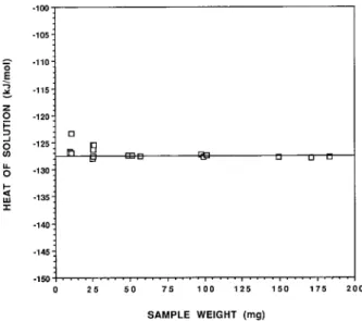
FIGURE2. Enthalpies of solution as a function of sample size for germanium oxide experiments of this investigation. The hor-izontal line represents an average heat of solution of2127.56 kJ/mol based on samples having weights greater than 49 mg.

Model 3497A) permitted virtually instantaneous switch-ing between current and voltage circuits, as well as be-tween heater and thermometer circuits. A computer-based system made possible the storage of large volumes of data that could be time-averaged. More recently we have re-placed our digital voltmeter (HP Model 3456A) with a higher precision model (HP Model 3458A) that adds two significant digits to the precision with which low-level voltages can be determined. Thus, the precision with which values of_DT now can be determined is improved

even further relative to those of earlier automation. In addition, we have obtained a highly precise electronic balance (Mettler Model AT201) that allows sample weight to be known to a higher degree of accuracy than before.

E

To test the degree to which these improvements have affected calorimetric precision and the minimum required sample size, we performed dissolutions on hexagonal ger-manium oxide [unit-cell parameters, a ₅ 4.9850 (60.0002) A˚ and c55.6476 (60.0002) A˚ )] as a function of sample size. Germanium dioxide (GeO2) is a good

sub-stance for such measurements, because it dissolves quick-ly, minimizing the correction to _DT for heat exchange

during the dissolution period. However any number of quick-dissolving substances, including feldspathoids, ze-olites, and hydroxides, would have been equally viable candidates for this study. The GeO2was unground,

com-monly a single chunk or two of material per experiment. Even with such coarse material, dissolutions generally were completed in 3 or 4 min.

As is normal in our work, each dissolution was con-ducted near 50 8C in 910.1 g (about a liter) of 20.1 wt%

HF under isoperibolic conditions, i.e., T of the surround-ings remains constant. In some cases, noted in Table 1, two dissolutions were made in the same acid solution. This had no detectable effect on the results, undoubtedly because of the high dilution of dissolved ions in the acid. Five weight classes of GeO2were studied, including

sam-ples of 166 (₆18), 100, 50, 25, and 10 mg.

C

Table 1 and Figure 2 record the results of our experi-ments. All weight classes produced the same average heats of solution within two standard deviations of the data. The collective average heat of solution of hexagonal GeO2 for the 166, 100, and 50 mg weight classes was

2127.56 ₆0.19 kJ/mol, shown as the horizontal line in Figure 2.

Even though average heats of solution for the five weight classes are essentially the same, there are differ-ences among them in the reproducibility of results (seen on Fig. 2), thus in standard deviation (last column of Ta-ble 1). For the three highest weight classes,₆1 full stan-dard deviation in the data constitutes just 60.08, 0.14, and 0.03%, respectively, of the observed heats of solu-tion. This is the same degree of reproducibility that we have observed with other quick-dissolving substances (e.g., leucite, analcime, and pollucite) since this study was completed. However, the corresponding percentages for the 25 and 10 mg weight classes are 60.9 and 1.3%, respectively. Even though this precision is less than for samples 50 mg and above, these still constitute relatively small uncertainties that are appropriate for many types of projects.

It is instructive to note the heat generated by the dis-solution of GeO2 on a weight basis, which is equal to

21220 J/g. In magnitude, this is significantly less than the corresponding heats of solution for many silicate min-erals. Alkali feldspars (Hovis 1988), plagioclase feldspars (Hovis 1997), muscovite-paragonite micas (Roux and Hovis 1996), nepheline-kalsilite (Hovis and Roux 1993), leucite, sodalite, and analcime (unpublished data) produce weight-based heats of solution that are about twice that of GeO2. The minimum weight requirements for these

compounds most likely will be even less than those for GeO2.

C

Hydrofluoric acid solution calorimetry has changed significantly in the past 15 years. Improved precision in measurement apparatus and techniques have resulted in the reduction of required sample size by two orders of magnitude relative to that of the early 1980s. Calorimetric temperature changes as small as 0.0038C associated with the dissolution of solids are now detectable and highly reproducible. [Hemingway and Robie (1977) show that even smaller values of_DT will be detectable for the

vir-tual instantaneous dissolution of liquids.] Although the minimum sample weight required for a project depends on the purpose of the project and the magnitudes of

en-934 HOVIS ET AL.: HF SOLUTION CALORIMETRY USING SMALL SAMPLES TABLE1. Calorimetric data for hexagonal germanium oxide

Exper. No. Sample weight (g) Temperature change during dissolution (8C) Mean solution temperature (8C) Calorimeter heat capacity I (J/deg) Calorimeter heat capacity II (J/deg) Heat of solution I (fromCpI) (kJ/mol) Heat of solution II (fromCpII) (kJ/mol) Average Hsoln (kJ) 61 Std dev (kJ) 61 Std dev (%) 149–184 mg samples 721 724* 733 0.17082 0.18355 0.14941 0.054015 0.057990 0.047184 50.036 50.041 49.995 3873.3 3870.3 3875.9 3875.0 3871.8 3876.5 2127.85 2127.64 2127.77 2127.90 2127.68 2127.78 2127.77 60.10 60.08% 100 mg samples 734 737 742* 0.09750 0.10118 0.09918 0.030675 0.031881 0.031337 50.004 49.997 49.991 3876.0 3874.0 3870.5 3875.8 3874.2 3871.6 2127.29 2127.42 2127.65 2127.28 2127.42 2127.68 2127.46 60.18 60.14% 50 mg samples 735* 738* 741 0.05679 0.04907 0.05163 0.017920 0.015480 0.016269 49.992 49.997 49.983 3871.5 3870.8 3874.0 3871.6 3871.1 3873.8 2127.52 2127.46 2127.42 2127.52 2127.47 2127.42 2127.47 60.04 60.03% 25 mg samples 736 0.02529 0.007897 50.000 3875.8 3876.1 2126.33 2126.34 2126.59 740* 743 751 752* 0.02509 0.02553 0.02587 0.02500 0.007794 0.008059 0.008027 0.007925 49.995 49.981 49.975 49.975 3870.4 3872.5 3873.1 3869.5 3871.7 3873.1 3873.0 3869.5 2125.50 2127.60 2125.45 2128.04 2125.55 2127.62 2125.44 2128.04 61.12 60.89% 10 mg samples 771 774* 775 776* 0.01052 0.00970 0.01070 0.00977 0.003210 0.003043 0.003359 0.003072 49.944 49.995 49.956 49.968 3872.0 3868.8 3872.9 3869.2 3871.3 3867.9 3872.7 3868.7 2123.31 2126.70 2126.92 2126.99 2123.29 2126.67 2126.91 2126.97 2125.97 61.65 61.31% Notes: Calorimetric heat capacity I is measured before dissolution, heat capacity II after dissolution. Raw values for all enthalpies of solution have been multiplied by 0.998 for reasons noted by Hovis and Roux (1993, p. 1116). In the last column ‘‘61 standard deviation (%)’’ gives 1 standard deviation expressed as a percentage of the average heat of solution.

* Dissolved in acid of the preceding experiment.

ergy that one is attempting to detect, as a general rule compounds generating heats of solution of 22000 J/g produce highest-quality results for sample sizes down to 25 mg per dissolution. For projects requiring less preci-sion, around 1–2%, the minimum required sample will be even lower, perhaps 5 mg. This reduction in required sample size makes possible many new projects, including those on high-pressure materials, which have not previ-ously been approachable by HF solution calorimetric investigation.

A

We are grateful for the support of this work by the Earth Sciences Division of the National Science Foundation through grant EAR-9613710. We thank William Carey, Alexandra Navrotsky, and especially Bruce Hemingway for their thoughtful reviews of this manuscript. Hilary Alberti helped produce Figure 1, and Joyce Hovis assisted with proofreading.

R

Hemingway, B.S. and Robie, R.A. (1977) Enthalpies of formation of low albite (NaAlSi3O8), gibbsite (Al(OH)3), and NaAlO2; revised values for DH0 andDG0 of some aluminosilicate minerals. Journal of Research

f,298 f,298

of the United States Geological Survey, 5, 413–429.

Hovis, G.L. (1974) A solution calorimetric and X-ray investigation of Al-Si distribution in monoclinic potassium feldspars. In W.S. MacKenzie and J. Zussman, Eds., The feldspars, p. 114–144. Manchester Univer-sity Press, Manchester, U.K.

(1988) Enthalpies and volumes related to K-Na mixing and Al-Si order/disorder in alkali feldspars. Journal of Petrology, 29, 731–763.

(1997) Hydrofluoric acid solution calorimetric investigation of the effect of anorthite component on enthalpies of K-Na mixing in feld-spars. American Mineralogist, 82, 149–157.

Hovis, G.L. and Roux, J. (1993) Thermodynamic mixing properties of nepheline-kalsilite crystalline solutions. American Journal of Science, 293, 1108–1127.

Robie, R.A. and Hemingway, B.S. (1972) Calorimeters for heat of solution and low-temperature heat capacity measurements. United States Geo-logical Survey Professional Paper 755.

Roux, J. and Hovis, G.L. (1996) Thermodynamic mixing models for mus-covite-paragonite solutions based on solution calorimetric and phase equilibrium data. Journal of Petrology, 37, 1241–1254.

Waldbaum, D.R. and Robie, R.A. (1971) Calorimetric investigation of Na-K mixing and polymorphism in the alkali feldspars. Zeitschrift fur Na- Kris-tallographie, 134, 381–420.

MANUSCRIPT RECEIVEDFEBRUARY10, 1998

MANUSCRIPT ACCEPTEDAPRIL3, 1998