HAL Id: hal-02975093
https://hal.archives-ouvertes.fr/hal-02975093
Submitted on 28 Oct 2020
HAL is a multi-disciplinary open access
archive for the deposit and dissemination of
sci-entific research documents, whether they are
pub-lished or not. The documents may come from
teaching and research institutions in France or
abroad, or from public or private research centers.
L’archive ouverte pluridisciplinaire HAL, est
destinée au dépôt et à la diffusion de documents
scientifiques de niveau recherche, publiés ou non,
émanant des établissements d’enseignement et de
recherche français ou étrangers, des laboratoires
publics ou privés.
Automated Species Recognition Using Convolutional
Neural Networks
Allison Hsiang, Anieke Brombacher, Marina Rillo, Maryline
Mleneck-vautravers, Stephen Conn, Sian Lordsmith, Anna Jentzen, Michael
Henehan, Brett Metcalfe, Isabel Fenton, et al.
To cite this version:
Allison Hsiang, Anieke Brombacher, Marina Rillo, Maryline Mleneck-vautravers, Stephen Conn, et
al.. Endless Forams: >34,000 Modern Planktonic Foraminiferal Images for Taxonomic Training and
Automated Species Recognition Using Convolutional Neural Networks. Paleoceanography and
Pa-leoclimatology, American Geophysical Union, 2019, 34 (7), pp.1157-1177. �10.1029/2019PA003612�.
�hal-02975093�
Training and Automated Species
Recognition Using Convolutional
Neural Networks
Allison Y. Hsiang1 , Anieke Brombacher2 , Marina C. Rillo2,3 ,
Maryline J. Mleneck‐Vautravers4 , Stephen Conn5, Sian Lordsmith5, Anna Jentzen6, Michael J. Henehan7 , Brett Metcalfe8,9 , Isabel S. Fenton10,11 , Bridget S. Wade12 , Lyndsey Fox3 , Julie Meilland13 , Catherine V. Davis14 , Ulrike Baranowski15, Jeroen Groeneveld16 , Kirsty M. Edgar15 , Aurore Movellan , Tracy Aze17, Harry J. Dowsett18 , C. Giles Miller3 , Nelson Rios19, and Pincelli M. Hull20
1Department of Bioinformatics and Genetics, Swedish Museum of Natural History, Stockholm, Sweden,2School of Ocean and Earth Science, National Oceanography Centre Southampton, University of Southampton, Southampton, UK, 3Department of Earth Sciences, Natural History Museum, London, UK,4Godwin Laboratory for Paleoclimate Research, Department of Earth Sciences, University of Cambridge, Cambridge, UK,5School of Earth and Ocean Sciences, Cardiff University, Cardiff, UK,6Department of Climate Geochemistry, Max Planck Institute for Chemistry, Mainz, Germany, 7GFZ German Research Centre for Geosciences, Potsdam, Germany,8Laboratoire des Sciences du Climat et de l'Environnement, LSCE/IPSL, CEA‐CNRS‐UVSQ, Université Paris‐Saclay, France,9Earth and Climate Cluster, Department of Earth Sciences, Faculty of Sciences, VU University Amsterdam, Amsterdam, The Netherlands, 10Department of Life Sciences, Natural History Museum, London, UK,11Department of Earth Sciences, University of Oxford, Oxford, UK,12Department of Earth Sciences, University College London, London, UK,13MARUM, Universität Bremen, Leobener Straße 8, Bremen, Germany,14Department of Earth and Planetary Sciences, University of California, Davis, CA, USA,15School of Geography, Earth and Environmental Sciences, University of Birmingham, Birmingham, UK, 16Alfred Wegener Institute, Helmholtz Center for Polar and Marine Research, Bremerhaven, Germany,17School of Earth and Environment, University of Leeds, Leeds, UK,18Florence Bascom Geoscience Center, U.S. Geological Survey, Reston, VA, USA,19Biodiversity Informatics and Data Science, Peabody Museum of Natural History, Yale University, New Haven, CT, USA,20Department of Geology and Geophysics, Yale University, New Haven, CT, USA
ABSTRACT
Planktonic foraminiferal species identification is central to many paleoceanographic studies, from selecting species for geochemical research to elucidating the biotic dynamics ofmicrofossil communities relevant to physical oceanographic processes and interconnected phenomena such as climate change. However, few resources exist to train students in the difficult task of discerning amongst closely related species, resulting in diverging taxonomic schools that differ in species concepts and boundaries. This problem is exacerbated by the limited number of taxonomic experts. Here we document our initial progress toward removing these confounding and/or rate‐limiting factors by generating thefirst extensive image library of modern planktonic foraminifera, providing digital taxonomic training tools and resources, and automating species‐level taxonomic identification of planktonic foraminifera via machine learning using convolution neural networks. Experts identified 34,640 images of modern (extant) planktonic foraminifera to the species level. These images are served as species exemplars through the online portal Endless Forams (endlessforams.org) and a taxonomic training portal hosted on the citizen science platform Zooniverse (zooniverse.org/projects/ahsiang/ endless‐forams/). A supervised machine learning classifier was then trained with ~27,000 images of these identified planktonic foraminifera. The best‐performing model provided the correct species name for an image in the validation set 87.4% of the time and included the correct name in its top three guesses 97.7% of the time. Together, these resources provide a rigorous set of training tools in modern planktonic foraminiferal taxonomy and a means of rapidly generating assemblage data via machine learning in future studies for applications such as paleotemperature reconstruction.
©2019. The Authors.
This is an open access article under the terms of the Creative Commons Attribution‐NonCommercial‐NoDerivs License, which permits use and distri-bution in any medium, provided the original work is properly cited, the use is non‐commercial and no modifica-tions or adaptamodifica-tions are made.
Key Points:
• We built an extensive image database of modern planktonic foraminifera with high‐quality species labels, available on an online portal
• Using this database, we trained a supervised machine learning classifier that automatically identifies foraminifera with high accuracy
• Our database and machine classifier represent important resources for facilitating future
paleoceanographic research using foraminifera Supporting Information: • Supporting Information S1 • Table S1 • Table S2 • Table S3 • Table S4 Correspondence to: A. Y. Hsiang, allison.hsiang@nrm.se Citation:
Hsiang, A. Y., Brombacher, A., Rillo, M. C., Mleneck‐Vautravers, M. J., Conn, S., Lordsmith, S., et al (2019). Endless Forams: >34,000 modern planktonic foraminiferal images for taxonomic training and automated species recognition using convolutional neural networks. Paleoceanography and
Paleoclimatology, 34, 1157–1177. https://doi.org/10.1029/2019PA003612 Received 21 MAR 2019
Accepted 7 JUN 2019
Accepted article online 23 JUN 2019 Published online 22 JUL 2019
1. Introduction
When a young naturalist commences the study of a group of organisms quite unknown to him, he is at first much perplexed to determine what differences to consider as specific, and what as varieties, for he knows nothing of the amount and kind of variation to which a group is subject; and this shows, at least, how very generally there is some variation.‐ C. Darwin, The Origin of Species, 1859, p. 50
The calcite tests of planktonic foraminifera provide a critical resource for paleoclimatological and paleocea-nographic research as they are often analyzed, using a variety of geochemical techniques, to reconstruct fun-damental values such as sea surface temperature, salinity, and atmospheric pCO2(Kucera, 2007; Schiebel
et al., 2018), in addition to being analyzed quantitatively as an assemblage. In most geochemical applica-tions, it is necessary to pick out specific species of a particular size range to control for differences in depth habitat, seasonality, and symbiont ecology, among others, that influence the geochemical composition of planktonic foraminiferal calcite (Birch et al., 2013; Edgar et al., 2017). Accurate identification of species is thus critical for generating reliable paleoceanographic and paleoclimatic information.
Accurate species identification is, however, a nontrivial task. Even among experienced workers, taxonomic agreement is achieved for only ~75% of individuals encountered (Al‐Sabouni et al., 2018; Fenton et al., 2018). There are several reasons for this. Planktonic foraminifera have highly variable morphologies with near‐continuous morphological gradations between closely related taxa (Aze et al., 2011; Poole & Wade, 2019). In some cases, like the historic“pachyderma‐dutertrei intergrade” (Hillbrecht, 1997), genetic analysis has revealed the existence of pseudo‐cryptic species between historically named morphological end‐ members (Darling et al., 2006). In other cases, morphological variation is unrelated to genetic differentiation (e.g., Trilobatus sacculifer; André et al., 2013) and may simply reflect the standing morphological variation in a species or species complex. Regardless, this variation requires the practitioner to demarcate species at some point along a morphological continuum. As a result, the circumstances of one's taxonomic training has a significant effect on the boundary conditions of the morphospace definition of a specific species that is used in practice. Different groups of taxonomists have developed different concepts for the morphological identity of species over time, with self‐trained taxonomists having the most divergent opinions of species identity (Al‐Sabouni et al., 2018). One potential reason for such diverging opinions is the limited number of published exemplar images for species in taxonomic references and online resources.
Here we have generated the largest image database of modern planktonic foraminifera species to date through the combined efforts of more than twenty taxonomic experts. This unprecedented data set is shared through several online portals with the aim of unifying taxonomic concepts and providing a shared taxo-nomic training tool. We then use supervised machine learning techniques to automate the identification of species from images. Supervised machine learning methods have previously been used to automate spe-cies identification for several microscopic taxa, including coccoliths (Beaufort & Dollfus, 2004), pollen grains (Gonçalves et al., 2016; Rodriguez‐Damian et al., 2006), phytoplankton (Sosik & Olson, 2007), hymenopter-ans (Rodner et al., 2016), diatoms (Urbánková et al., 2016), and dipterhymenopter-ans and coleopterhymenopter-ans (Valan et al., 2019). However, these techniques have only been applied in a limited way (i.e., few species, low sampling, limited image variability, and scope) to modern planktonic foraminifera (Macleod et al., 2007; Mitra et al., 2019; Ranaweera et al., 2009; Zhong et al., 2017), preventing their use as a general tool in this field. Computer vision provides a way to not only automate a task that relatively few researchers are trained to do (i.e., identify all species in a sample) but to also ensure a level of consistency and, at times, accuracy that can be difficult to achieve with human classifiers due to subjectivity and/or bias.
2. Background on Supervised Machine Learning
Thefield of computer vision involves training computers to parse the content of visual information and is a core aspect of many artificial intelligence applications such as facial recognition and medical image analysis. A common computer vision task is identifying objects in 2‐D images using a set of previously‐identified images (i.e., a training set). The use of a training set in such tasks is called“supervised machine learning” and allows the computer to build a model of how an input (i.e., an image) maps to a categorical output (i.e., the identity or“class” of that image). To do this, the machine learning algorithm must determine what attributes of the input data are relevant for the prediction task at hand. This process is called feature
extraction and is a form of dimensionality reduction that transforms complex data into a set of explanatory variables that are grouped using similarity or distance metrics. The resulting model is called a“classifier.” The accuracy of a classifier is typically tested with a small set of known images, called a “test set” or “valida-tion set,” before it is used to predict the identity of unknown images (i.e., to assign classes to new input objects).
Artificial neural networks (ANNs) are the key building block for modern computer vision systems. ANNs consist of a collection of “neurons” (i.e., nodes) and edges that connect these neurons. If there is a connection between two neurons, then the output of thefirst neuron serves as input for the second neuron. Every connection has an associated weight that signifies the relative importance of the input. A neuron performs a computation on the weighted sum of its inputs. This computation is known as an activation function—for instance, a commonly used activation function is the Rectified Linear Unit (ReLU), which applies the transformation f(x) = max(0,x) (equivalent to replacing negative values with 0). The output of the neuron is then passed along to the other neurons to which it is connected. The neural networks used in computer vision are generally feed forward networks, whereby neurons are arranged in layers and all connectionsflow in a single (forward) direction. In other words, neurons in the same layer have no connections with one another. Instead, they only have connections with neurons in adjacent layers, receiving inputs from the preceding layer and sending outputs to the following layer. The most commonly used type of feed‐forward ANN is the multilayer perceptron, also known as a fully connected layer. As its name suggests, every neuron in a fully connected layer has connections to every neuron in the preceding layer.
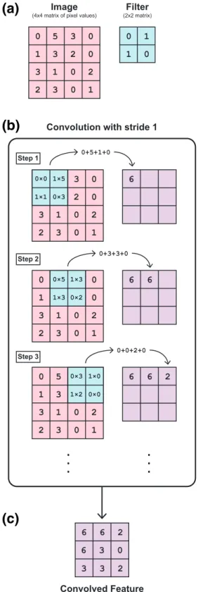
The current best performing algorithms for feature extraction and image classification use convolutional neural networks (CNNs; Krizhevsky et al., 2012; Hertel et al., 2017). CNNs build upon ANNs by including layers that perform convolution operations, which serve to extract features from input images. Any image can be represented as a matrix of pixel values. Convolution operations use these pixel values to calculate new values using element‐wise matrix multiplication with a small matrix (aka a “filter” or “kernel”) that sweeps over original image pixel values (Figure 1). The sums of the element‐wise multiplications (i.e., the dot product of thefilter values and the pixel values of the portion of the image the filter is currently placed over) then form the elements of a new matrix of convolved features (also known as an“activation map” or “feature map”). Examples of convolution operations include edge detection, sharpening, and blurring. As convolution operations are linear, a ReLU layer is usually applied following convolution in order to intro-duce nonlinearity into the network. This step is important because a simple linear function is limited in its ability to capture complex mappings between the input (images) and output (classes). Although other nonlinear activation functions exist, ReLU has been shown to perform better in most situations (Nair & Hinton, 2010). Following the convolution and ReLU layers are pooling layers that are used to perform down-sampling (i.e., dimension reduction), removing extraneous features while retaining the most relevant infor-mation. Commonly used pooling operations include max pooling (whereby the highest value in a neighborhood of pixels is retained and all others discarded) and average pooling (whereby the average of all values in a neighborhood of pixels is calculated and retained).
Combined, the convolution, ReLU, and pooling layers comprise the feature extraction portion of the CNN, producing as output the high‐level features that are then used to perform classification. The values com-puted by the network are then processed using fully connected layers, generating a vector of probabilities reflecting the probability that a given image falls in any given class. This complete process (from input to fea-ture extraction to classification) is known as forward propagation.
The training set provides the CNN with known examples of the correct mapping between image values and weights and thefinal classification (i.e., the true probability vector). When the CNN is initialized, all weights andfilters are randomly assigned. The network then takes the input images and runs the first forward pro-pagation step. As the weights andfilters are random at this point, the output is a vector of random class prob-abilities for each image. The total error (i.e., the sum of the differences between the true probability vector and the output probability vector) is calculated. The network then performs backpropagation, which is the process of updating all the weights andfilters using gradient descent in order to minimize the total error. One complete forward propagation and backpropagation of the entire data set is called an epoch. Ideally, all images would be passed through the neural network at once to result in the most accurate backpropagation
Figure 1. Example of how convolution is performed in a convolutional neural network. (a) An image can be represented as a matrix of pixel (px) values. Here we have a 4px by 4px image represented as a 4 × 4 matrix. We use an examplefilter, or kernel, that is represented by the 2 × 2 matrix shown. (b) Convolution is performed by sweeping thefilter across the image and summing the resulting values from element‐wise multiplication of the values of the image matrix that the filter overlaps with the correspondingfilter values. These sums are then saved to a new matrix that has one entry for every step of the convolution process. Here we use a stride of 1px, meaning that thefilter moves 1px in each step. This is repeated until thefilter has been passed over the entire image. (c) The resulting matrix of sums is the convolved feature, also known as an“activation map” or “feature map.”
updates possible. However, in practice, this is computationally intractable, and the data must be broken up into separate smaller batches to feed into the network. In general, the larger the batch size, the better. However, the maximum batch size is limited by the amount of memory available to hold all of the data at once. The number of batches required to complete a single epoch is called the number of iterations. For example, a data set containing 1,000 images could be split intofive batches of 200 images. Training a CNN using this data set would then takefive iterations to complete one epoch. The number of epochs required to adequately train a network is variable and depends on the characteristics of the data set and the parameters associated with the gradient descent algorithm being used.
By updating weights and kernels in the backpropagation to reduce classification error, the network learns how to accurately classify the training images, building an association between a particular collection of weights and kernels and a particular output class. The best‐performing model is then used to classify the images in the validation data set. The performance of the model on the validation set thus gives us an idea of how well the model performs, and what sort of accuracies we might expect if the model was used to clas-sify entirely novel images. Model performance is evaluated by looking at validation accuracy (i.e., the pro-portion of images in the validation set that are correctly identified by the trained model) and validation loss (i.e., the sum of errors for each image in the validation set, where error is determined by a loss function such as cross‐entropy; see supporting information Text S2).
The 16‐layer VGG16 (named after the Visual Geometry Group at Oxford University) CNN (Simonyan & Zisserman, 2014) is a commonly used image classification neural network. Although VGG16 is a relatively shallow network, its development was critical in showing that, in general, the deeper a neural network (i.e., the more layers it contains), the more accurate its performance. However, training difficulty and computa-tional costs (i.e., time) increase with neural network depth. Residual Networks (ResNets; He et al., 2015) and Densely Connected Convolutional Networks (DenseNets; Huang et al., 2016) are state‐of‐the‐art CNNs that have helped alleviate this computational cost and improve performance. ResNets and DenseNets containing hundreds of layers are now possible. However, no algorithm is universally ideal for all machine learning pro-blems (Wolpert & Macready, 1997). A certain amount of experimentation with algorithm choice is thus a necessity. Training deep CNNs also requires extremely large amounts of data to meaningfully infer values for the large number of model parameters (and, correspondingly, computational resources). As a result, dee-per networks may not necessarily be preferable for all problems.
One technique that eases computational burden and allows for robust models to be trained using relatively small data sets is called transfer learning. Transfer learning uses weights from a model previously trained using another data set on a new task; these weights are“frozen” in the new model so that they are not train-able, thus reducing the number of parameters that must be estimated. New images are then used only to train the unfrozen layers at the end of the CNN in order tofine‐tune the model to the task at hand. This can be an efficient and effective strategy when one does not have a very large data set with which to train a CNN from scratch. For example, ImageNet, which contains over 14 million images of various objects and activities, has been used to train many CNNs, and the resulting weights are freely available. Transfer learning thus allows accurate models to be trained with hundreds to thousands, rather than millions, of images.
In this study, we generate a large image data set of planktonic foraminifera with associated high‐quality spe-cies labels assigned by taxonomic experts. We then use these data to train a supervised machine learning classifier using deep CNNs that is able to automatically identify planktonic foraminifera with high accura-cies that are comparable to those of human experts.
3. Methods
Planktonic foraminiferal images were obtained from two large databases: a North Atlantic coretop collection from the Yale Peabody Museum (hereafter, YPM Coretop Collection) and the Henry A. Buckley collection from the Natural History Museum, London (hereafter, Buckley Collection).
3.1. Species Identification of the YPM Coretop Collection
The YPM Coretop Collection is a data set of 124,230 object images collected by Elder et al. (2018) from the ≥150‐μm size fraction of 34 Atlantic coretop samples. Of these objects, 61,849 were identified as complete
or damaged planktonic foraminifera by human classifiers. To identify these images to the species level, we used the online platform Zooniverse to create a private portal for taxonomic experts to identify images. As several taxonomies exist for extant planktonic foraminifera, we standardized the species list by using the SCOR/IGBP Working Group 138 taxonomy (Hottinger et al., 2006). Further details regarding the Zooniverse interface and data collection are available in the supporting information.
To collect statistics on classifier accuracy and avoid inaccurate labels resulting from single‐user errors, four independent taxonomists classified each image before it was considered complete. Classifiers were required to identify each image they encountered. They were not permitted to respond with“I do not know” and were advised to not skip images (although this was possible by refreshing the page). This is because the classi fica-tions themselves made difficult‐to‐classify individuals apparent, as the truly unidentifiable individuals were unlikely to be called the same thing by four independent experts. Additionally, even uncertain responses can provide useful information. For example, if the three labels assigned to an individual were“Globigerinoides
ruber,” “Globigerinoides elongatus,” and “Globigerinoides conglobatus,” it is very likely that the individual belongs to the genus Globigerinoides, although the exact species identity of the individual is ambiguous. An email was sent to the planktonic foraminiferal community to invite self‐identified experts to the project. A total of 24 taxonomists submitted at least one classification and of these, 16 submitted more than 5,000 classifications and are co‐authors on this manuscript. In sum, 140,616 unique classifications were collected on the 40,000 unique images uploaded. The raw data was processed to determine how many objects received four independent classifications, and what degree of agreement existed between the independent object clas-sifications. All objects with 75% agreement or higher were considered to have high‐quality classifications and were retained for CNN training and validation. Thefinal set of YPM Coretop Collection images with high‐quality species labels includes representatives from 34 species and comprises a total of 24,569 individuals.
3.2. Species Identification of the Buckley Collection
We included images of planktonic foraminifera from the Henry A. Buckley collection at the Natural History Museum in London, which includes samples from various localities worldwide, primarily from the Pacific, Atlantic, and Indian oceans (see Rillo et al., 2016, for details regarding the Buckley specimens). A total of 1,355 slides containing identified modern specimens were segmented using AutoMorph (Hsiang et al., 2017; available at https://github.com/HullLab/AutoMorph) for inclusion in the machine learning data set. All slides were segmented using an object size range of 50‐800 pixels and a test threshold value range of 0.5–0.7, incremented by 0.01, resulting in 30 segmentations per slide. The segmentation results were exam-ined by eye to determine the ideal threshold value that maximizes the number of correctly identified forami-nifera and minimizes the number of spurious objects segmented by the algorithm. A total of 17,383 objects were segmented out of the 1,355 modern slides.
After segmentation, A. B. and M. C. R. examined all segmented objects using a modified version of the Specify software (Hsiang et al., 2016) in order to (1)flag spurious identified objects for removal (usually bits of background or slide labels) and (2) mark whether the original species identification provided by Buckley matched modern species concepts unambiguously. Objects for which both A. B. and M. C. R. agreed with Buckley's original label were retained for thefinal image data set, resulting in a total of 10,071 images. For certain species, Buckley used antiquated names that mapped unambiguously onto modern synonyms; these names were updated to follow the SCOR taxonomy (Table S1), and the species images were included in thefinal data set. The final Buckley data set includes representatives from 31 species, two of which (Globigerinella adamsi and Tenuitella iota) are not found in the YPM data set.
3.3. Supervised Machine Learning
Following convention, we withheld 20% of the combined YPM + Buckley data set as a test data set (i.e., vali-dation set), with the remaining 80% used for training. For the YPM data set, 20% of the data set had already been designated as withheld objects during data set creation (see Elder et al., 2018). We used this list to split those images with high‐quality species labels into a test set (i.e., all images with originally “withheld” object IDs) and a training set. This resulted in 4,889 test objects and 19,680 training objects (24,569 objects total). For the Buckley data set, 20% of the 10,071 images (2,014 total) were randomly selected to be part of the test set. The remaining images (8,057 total) comprised the training set. We then merged the YPM and Buckley
data sets. This merged data set contains 34,640 images total, with a training set of 27,737 images and a test set of 6,903 images. A total of 35 species (+1“Not a planktonic foraminifer” option = 36 total classes) are repre-sented. Table S2 contains a breakdown of the number of representatives by species in the training set. Our sampling represents ~73% coverage of the 48 total species defined in the SCOR taxonomy, with the missing species being either extremely rare or typically smaller than the size fraction imaged and classified here. We initially tested three CNNs: VGG16 (Simonyan & Zisserman, 2014), DenseNet121 (Huang et al., 2016), and InceptionV3 (Szegedy et al., 2015). These CNNs are commonly used neural networks for image classi fi-cation. We used the implementation of these CNNs from the Keras Python API (Chollet et al., 2015) using the GPU‐enabled TensorFlow (Abadi et al., 2016) backend. Details on all model structures and analysis para-meters can be found in Text S2 of the supporting information. Table 1 summarizes all supervised machine learning analyses that were run. Treatments and parameter values were optimized iteratively, with the opti-mally performing value retained from each testing cycle for the next. For instance, wefirst tested the effect of image size on accuracy by holding all other treatments and parameter values constant (analyses 1–3 in Table 1). As an image size of 160 × 160 pixels yielded the highest validation accuracy, we set the image size to 160 × 160 pixels for all remaining analyses. We performed these tests in the following order: image size, dropout, learning rate, L1/L2 regularization, augmentation, and batch size (see supporting information Text S2). For thefinal analyses, we also increased the patience value of the early stopping algorithm to 10. All ana-lyses were run on the Beella machine in the Hull Lab in the Department of Geology and Geophysics depart-ment at Yale University (6‐core 2.4GHz CPU, 32 GB RAM, 2 NVIDIA GeForce GTX 1080 GPUs [8 GB], Ubuntu 15.04.5 LTS). The code for the machine learning analyses is available on GitHub (https://www. github.com/ahsiang/foram‐classifier).
3.4. Taxonomic Training Tools and Resources
The 32,626 training set images are available through the website Endless Forams (endlessforams.org). This website was designed to deliver as many species examples as a user requests, up to the total number of images available for a species, for taxonomic training purposes. By looking at many, or all, of the images available for any given species, researchers will be able to gain an understanding of the extent of morpholo-gical variability that is generally accepted amongst taxonomists within any given species. We have also designed an extensive taxonomic training portal (available at endlessforams.org) for workers that utilizes the training set images. Users can then use the public‐facing Zooniverse portal (zooniverse.org/projects/ ahsiang/endless‐forams) to participate in classifying the >14,000 remaining unclassified planktonic forami-nifera images from the YPM Coretop Collection. Because this new Zooniverse portal is public‐facing, all images require 15 identifications before being retired and considered fully “classified.” The portal will be monitored regularly, and any retired images with <75% agreement will be reuploaded to the portal, until eventually the only images left in the portal will be the truly ambiguous, unclassifiable objects.
4. Results
4.1. Expert Species Identification
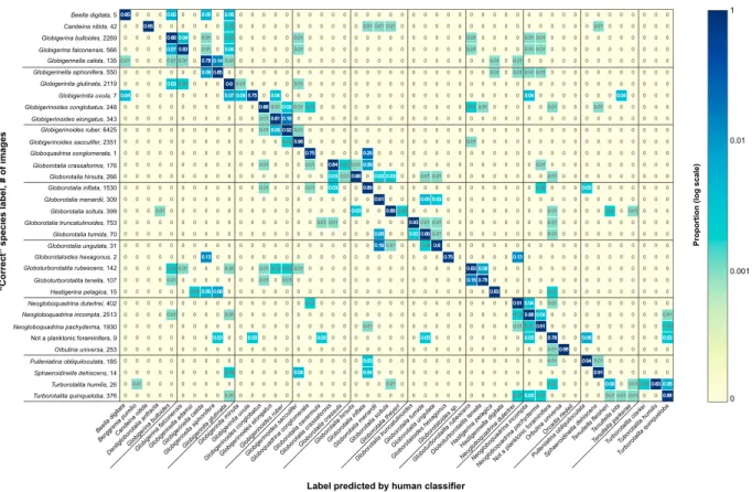
A total of 34,067 images were fully identified (i.e., four classifications obtained) from the YPM Coretop Collection, of which 1,604 (4.71% of the total) had 0% agreement (i.e., all four identifiers disagreed on the species identification), 7,894 (23.17%) had 50% agreement, 9,578 (28.12%) had 75% agreement, and 14,991 (44.00%) had 100% agreement. This resulted in a data set of 24,569 unique images (72.12% of the total data set) with high‐quality labels (i.e., three or four of four identifiers agreed on the classification), representing 34 species. A human confusion matrix (Figure 2) was generated using the objects with high‐quality labels by summing the number of identifications for each of the 34 species and determining the proportion of the iden-tifications are correct or incorrect. For instance, the final data set contained 343 images that were identified as Globigerinoides elongatus. These images required a total of 1,372 identifications (=343 × 4), of which 81% were the“correct” identification (i.e., G. elongatus). The remaining 19% of identifications were incorrect, with most being G. ruber (18%) and the rest being G. conglobatus (1%). In general, most of the classifications are correct, with accuracy rates ranging from 75% to 98% (average accuracy: 85.9%), as only those individuals with 75% agreement or more were considered“identified.” Species with accuracy rates ≤80% were relatively rare in the data set as well: Globigerinella calida: 78% accuracy, 135 individuals; Globigerinita uvula: 75%, 7 individuals; Globorotalia ungulata: 80%, 31 individuals; Globorotaloides hexagonus: 75%, 2 individuals;
Table 1
Supervised Machine Learning Analyses
Analysis Number CNN used Image size (pixels) Batch size Layers frozen Dropout Dropout
value Learning rate
Adjustment factor L1/L2 regularization Lambda value 1 VGG16 64 × 64 100 7 No ‐ 0.0001 ‐ No ‐ 2 VGG16 96 × 96 100 7 No ‐ 0.0001 ‐ No ‐ 3 VGG16 128 × 128 100 7 No ‐ 0.0001 ‐ No ‐ 4 VGG16 160 × 160 100 7 No ‐ 0.0001 ‐ No ‐ 5 VGG16 160 × 160 100 7 Yes 0.1 0.0001 ‐ No ‐ 6 VGG16 160 × 160 100 7 Yes 0.01 0.0001 ‐ No ‐ 7 VGG16 160 × 160 100 7 Yes 0.5 0.0001 ‐ No ‐ 8 VGG16 160 × 160 100 7 Yes 0.9 0.0001 ‐ No ‐ 9 VGG16 160 × 160 100 7 Yes 0.5 0.001 ‐ No ‐ 10 VGG16 160 × 160 100 7 Yes 0.5 0.00001 ‐ No ‐ 11 VGG16 160 × 160 100 7 Yes 0.5 0.00005 ‐ No ‐ 12 VGG16 160 × 160 100 7 Yes 0.5 0.0001 ‐ Yes 0.01 13 VGG16 160 × 160 100 7 Yes 0.5 0.0001 ‐ Yes 0.0001 14 VGG16 160 × 160 100 7 Yes 0.5 0.0001 ‐ Yes 0.00001 15 VGG16 160 × 160 100 7 Yes 0.5 0.0001 ‐ Yes 0.0000001 16 VGG16 160 × 160 100 7 Yes 0.5 0.0001 ‐ No ‐ 17 VGG16 160 × 160 100 7 Yes 0.5 0.0001 ‐ No ‐ 18 VGG16 160 × 160 100 7 No ‐ 0.0001 ‐ No ‐
19 VGG16 160 × 160 100 7 Yes 0.5 Self‐regulating 0.9 No ‐
20 VGG16 160 × 160 100 7 Yes 0.5 Self‐regulating 0.5 No ‐
21 VGG16 160 × 160 200 7 Yes 0.5 Self‐regulating 0.5 No ‐
22 VGG16 160 × 160 250 7 Yes 0.5 Self‐regulating 0.5 No ‐
23 VGG16 160 × 160 200 7 Yes 0.5 Self‐regulating 0.5 No ‐
24 InceptionV3 139 × 139 100 249 Yes 0.5 0.0001 ‐ No ‐ 25 DenseNet121 299 × 299 100 313 Yes 0.5 0.0001 ‐ No ‐ Analysis number Augmentation Num. Aug. treatments Early‐stopping patience Epochs ran Max. training accuracy Min. training loss Max. validation accuracy Min. validation loss 1 No ‐ 5 15 0.97 0.08 0.79 0.77 2 No ‐ 5 11 0.95 0.13 0.80 0.66 3 No ‐ 5 32 0.99 0.03 0.83 0.63 4 No ‐ 5 32 0.99 0.03 0.85 0.63 5 No ‐ 5 19 0.98 0.05 0.84 0.56 6 No ‐ 5 29 0.99 0.03 0.84 0.59 7 No ‐ 5 27 0.99 0.04 0.86 0.55 8 No ‐ 5 30 0.98 0.07 0.83 0.76 9 No ‐ 5 40 0.84 0.46 0.73 0.93 10 No ‐ 5 27 0.97 0.11 0.85 0.55 11 No ‐ 5 17 0.98 0.07 0.84 0.56 12 No ‐ 5 18 0.21 2.94 0.23 2.94 13 No ‐ 5 15 0.97 0.15 0.80 0.81 14 No ‐ 5 15 0.97 0.12 0.82 0.65 15 No ‐ 5 15 0.97 0.08 0.84 0.60 16 Yes 5 5 14 0.90 0.31 0.82 0.59 17 Yes 2 5 24 0.96 0.11 0.84 0.58 18 Yes 2 5 10 0.91 0.27 0.81 0.58 19 No ‐ 5 23 0.99 0.02 0.85 0.57 20 No ‐ 5 28 1.00 2.00 × 10⁻⁴ 0.87 0.59 21 No ‐ 5 35 1.00 6.00 × 10⁻⁴ 0.86 0.61
Globoturborotalita tenella: 78%, 107 individuals; and Globoquadrina conglomerata: 75%, 1 individual). In most cases, misidentifications occurred within the same genus, although these misidentifications are not necessarily symmetrical. For instance, while G. elongatus is misidentified as G. ruber 18% of the time, the reverse happens only 5% of the time.
Table S3 shows anonymized user accuracy rates. The range for user accuracies of high‐quality labels (i.e., the proportion of correct labels each user contributed, for all objects with 75% or 100% agreement) was 63.8%–85.2%.
4.2. Supervised Machine Learning Model Training
Although we began by testing the VGG16 (analysis #1 in Table 1), InceptionV3 (analysis #24), and DenseNet121 (analysis #25) CNN architectures, it quickly became clear that the latter two networks were affected by strong overfitting, as the validation accuracy was always significantly lower than the training
Figure 2. The human confusion matrix, showing results from 24,569 individuals from the YPM coretop data set with high‐quality (i.e., ≥75% classifier agreement) species labels. The y axis lists the species comprised by the high‐quality (or correct) identifications, followed by the number of images representing that species. The
xaxis is the list of all species that objects were potentially identified as. Each cell of the matrix represents the proportion of identifications for each species (y axis) that are identified as the corresponding species on the x axis (e.g., 88% of the IDs collected for the 2,269 images of G. bulloides were correct and 4% of those IDs were incorrectly selected to be G. falconensis). The color map is on a log‐scale and shows higher (bluer/darker) versus lower proportions (yellower/lighter).
Analysis number Augmentation Num. Aug. treatments Early‐stopping patience Epochs ran Max. training accuracy Min. training loss Max. validation accuracy Min. validation loss 22 No ‐ 5 32 1.00 2.00 × 10⁻³ 0.86 0.62 23 No ‐ 10 44 1.00 3.00 × 10⁻⁴ 0.87 0.56 24 No ‐ 5 20 1.00 1.2 × 10⁻³ 0.48 1.84 25 No ‐ 5 16 1.00 0.04 0.34 2.52
accuracy. Due to these preliminary results, we decided to move forward with the VGG16 CNN, as it does not experience the same degree of model overfitting that we observed with DenseNet121 and InceptionV3 and also exhibited the highest initial validation accuracy (78.96%).
Our results show a positive effect of image size on validation accuracy at low pixel counts (analyses #1–4 in Table 1) with validation accuracy increasing from 78.96% at 64 × 64 pixels to 84.77% at 160 × 160 pixels. As training accuracy, training loss, and validation loss do not improve appreciably between an image size of 124 × 124 pixels versus 160 × 160 pixels, we chose to cap the image size at 160 × 160 pixels, as increasing image size requires a corresponding increase in memory usage and processing time. Next, we tested the effect of adding dropout regularization with different dropout proportions (analyses #5–8). The best performing ana-lysis had a dropout value of 0.5, which resulted in a validation accuracy of 85.59%. For the learning rate tests (analyses #9–11), a relatively high learning rate of 0.01 resulted in the lowest validation accuracy (72.80%). As the lower learning rates of 1.0 × 10⁻⁵and 5.0 × 10⁻⁵did not result in higher validation accuracies than the intermediate rate of 1 × 10⁻⁴, we retained an intermediate rate for the following analyses, as low learning rates can lead to slow convergence. L1/L2 regularization (analyses #12–15) also did not improve validation accuracies, and in fact, a lambda value of 0.01 resulted in a precipitous drop in both training and validation accuracy (21.40% and 22.93%, respectively). We thus chose to proceed without the use of L1/L2 regularization.
We compared data augmentation usingfive versus two treatments (analyses #16–17) and found that while the two‐treatment method performed better than the five‐treatment method (validation accuracy of 84.36% versus 82.35%), neither resulted in substantially increased validation accuracy than the analyses without data augmentation. Because data augmentation is a form of regularization, it can sometimes lead to under-fitting when used in combination with other regularization techniques such as dropout and L1/L2 regular-ization. As such, we also tested the effect of the two‐treatment data augmentation without the 0.5 dropout layer (analysis #18). However, this resulted in a lower validation accuracy of 81.07%. We thus decided to retain the dropout regularization without the data augmentation, as dropout appears to have the greatest effect in reducing overfitting in our data set. We then tested a self‐adjusting learning rate and found that it led to a significantly improved validation accuracy of 87.32% in the 0.5 adjustment factor case (analysis #20). Finally, we found that increasing the batch size to 200 and 250 (analyses #21–22) led to relatively high validation accuracies (>85%) and very high training accuracies (>99%) and low loss (6.0 × 10⁻⁴–2.0 × 10⁻³). Thefinal analysis (#23) combining the best performing settings resulted in a training accuracy of 99.99%, a training loss of 3.0 × 10⁻⁴, a validation accuracy of 87.41%, and a validation loss of 0.5638. We also calculated the proportion of objects for which the correct species identity is found within the top three guesses made by the model (i.e., the top‐3 accuracy) and found a last run top 3 training accuracy of 100% and a top 3 validation accuracy of 97.66%. Figure 3 shows the evolution of all these metrics through the 44 epochs that thisfinal analysis was trained. Thefinal model weights, along with the code used for training and validation, can be accessed at https://www.github.com/ahsiang/foram‐classifier website.
The machine confusion matrix is shown in Figure 4. Some differences in the general pattern of misidentifi-cations between the machine and human confusion matrices present themselves. While the human misi-dentifications tend to be phylogenetically conservative (i.e., when individuals are misidentified, they are usually misidentified as another species from the same genus), the misidentifications by the machine are more liberal—for instance, 21% of the validation specimens of Globigerinella calida are misidentified as
Globigerina falconensis. The model tended to confuse species in this manner when they have relatively low sampling: the average training sample size of species with validation accuracies <70% is 130, compared with an average training sample size of 1,184 for those species with validation accuracies >70%. The accu-racy of human classifiers versus the machine model on the validation set for each species is shown in Figures 5a–5b.
Another interesting result is that Globorotalia ungulata is correctly identified by the machine only 33% of the time and mistaken as Globorotalia menardii the other 67% of the time. It is the only species that is always misidentified as a single alternate species at a greater frequency than it is correctly identified. Human iden-tifiers also commonly misidentify G. ungulata as G. menardii (18% misidentifications), and the machine is likely further misled due to the much larger set of training images for G. menardii than for G. ungulata (1,090 vs. 25; see Discussion on the class imbalance problem, below).
5. Discussion
5.1. Building and Mobilizing Large‐Scale Taxonomic Resources
Zooniverse was an effective platform for obtaining taxonomic identifications on digital images from experts. Given the paucity of images available for planktonic foraminiferal species, it is noteworthy that this project generated >34,000 identifications in just three months. Large‐scale digital mobilization efforts like this one provide one means of capturing our community expertise for training the next generation of scientists and for automating some aspects of our work. As we show below, once generated, large‐scale data products such as these can be used to automate future classification tasks through machine learning. The portals we pro-vide for both the raw images (endlessforams.org) and taxonomic training (zooniverse.org/projects/ahsiang/ endless‐forams) are targeted toward increasing the expertise and consistency of single (or limited)‐taxon experts (e.g., many geochemists), as well as taxonomists, by illustrating the range of variation accepted in each species concept (Figure 6) and providing a common benchmark to reduce differences amongst taxonomic schools.
In general, we would repeat the same portal design for future projects with the following exceptions. Given the difficulty of taxonomic identification from digital images (i.e., taxonomists like to rotate specimens to see
Figure 3. Plots showing evolution of top 1 accuracy, loss, and top 3 accuracy with epoch number during model training using the VGG16 CNN with an image size of 160 × 160 pixels, a batch size of 200, 0.5 dropout regularization, a self‐adjusting learning rate with an adjustment factor of 0.5, and early stopping with a patience of 10. A total of 44 epochs were completed before the early stopping algorithm stopped the run. The maximum top 1 training accuracy was 99.99%; the maximum top 1 validation accuracy was 87.41%; the minimum training loss was 0.0003; the minimum validation loss was 0.5638; the maximum top 3 training accuracy was 100%; and the maximum top 3 validation accuracy was 97.66%.
key taxonomic features), partial occlusion by sediment or poor preservation made species‐specific identification very difficult. Methods for dealing with poor preservation in the context of digital data mobilization includefiltering out poorly‐preserved samples or sites or classifying at the generic rather than species level. We also had remixing in some samples, and because we did not include a“remixed” option for classifiers, experts were forced to assign modern names to ancient taxa in these instances. A remixed option, along with the existing not a planktonic foraminifer option, will be included in all future studies.
The human by‐user accuracy rates that we observe (63.8%–85.2%; average 71.4%) are well in line with those reported by previous studies on the performance of human classifiers on large‐scale taxonomic identification tasks. In a study on species identification of six species of Dinophysis dinoflagellates, Culverhouse et al. (2003) report an average accuracy rate of 72% amongst 16 taxonomic experts. A study examining expert versus nonexpert performance on species identification in bumblebees found accuracy rates of below 60% for both groups (Austen et al., 2016). Finally, Al‐Sabouni et al. (2018) report average accuracies of 69% (>125‐μm size fraction) and 77% (>150‐μm size fraction) in a study of 21 experts identifying 300 plank-tonic foraminifera specimens from slides, with a 7% drop in accuracy between slides and digital photos. The high level of accuracy found by Al‐Sabouni et al. is notable, given the widely held perception that
Figure 4. The machine confusion matrix, showing results from the validation set, which contains 80% of the images with high‐quality labels from the combined YPM coretop data set and the Buckley data set. The y axis shows the“correct” species labels followed by the number of representative images in the validation set. The x axis shows the corresponding predicted labels, with each matrix cell showing the proportion of validation objects identified as each species (e.g., 86% of the 536 validation images of G. bulloides were correctly identified as G. bulloides and 4% were incorrectly identified as G. falconensis). The color map is on a log‐scale and shows higher (bluer/darker) vs. lower proportions (yellower/lighter).
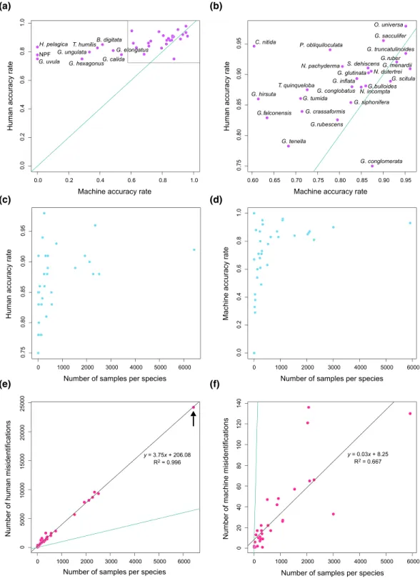
Figure 5. Cross‐plots comparing machine and human classifier performance. (a) Comparison of machine accuracy rates (i.e., proportion of validation images cor-rectly identified) versus human accuracy rates (i.e., proportion of correct identifications out of all identifications collected for the objects with high‐quality species labels).“NPF” = Not a Planktonic Foraminifera. (b) Close‐up of the box in panel (a). (c) Relationship between the number of samples per species and the human accuracy rate. (d) Relationship between the number of training samples per species and the machine accuracy rate. (e) Plot showing the relationship between the number of specimens sampled per species and the total number of human misidentifications that fall in that species category. For instance, the point marked with the arrow represents Globigerinoides ruber, which has 6,425 representatives in the data set. Of all the identifications scored for the other 33 species in the data set, a total of 24,202 of identifications are mistakenly scored as G. ruber. There is a strong correlation (R2= 0.996; p < 2.2 × 10⁻¹⁶) between the number of representative specimens per species and the total number of misidentifications that fall into that species category. (f) Analogous plot to (e) but for the machine validation set and misidentifications. The correlation between the number of representative samples for a class and the number of misidentifications that fall in that class is much weaker for the machine classifier (R2= 0.667; p = 1.253 × 10⁻⁹) than for the human classifiers. The green line in all plots represents the identity line.
planktonic foraminifera have intergrading morphologies. In contrast, Mitra et al. (2019) report classification performances for six experts (>15 years of experience) and novices (0.5–2 years of experience) identifying 540 specimens andfind F1 scores (harmonic mean of precision and recall) of 39%–85% (mean 63%) for experts and 47%–64% (mean 53%) for novices. The relatively lower accuracies reported by Mitra et al. may result from the option classifiers were given to choose “Not Identifiable,” which may cause conservative classifiers to avoid making decisions if they are uncertain, leading to depressed recall rates (i.e., more false negatives). Furthermore, as the original identities of the images used by Mitra et al. were determined by only a single expert, the accuracy rates are dependent on the accuracy of this original expert. The“true” identities of the specimens used in our study are determined from the aggregate classifications of four independent, random classifiers per specimen. As these experts may have differing species concepts, we can be reasonably certain in identifications that have ≥75% agreement, because the majority of experts
Figure 6. Plates showing examples of the range of morphological, preservational, and imaging (orientation, color, lighting, etc.) variation within a given species in the Yale data set. Representatives from four example species (Globigerinoides ruber, Globigerina bulloides, Orbulina universa, and Globorotalia menardii) are shown here. The pink specimen of G. bulloides comes from a slide where all specimens had been stained with Rose Bengal.
agree on the identity despite these differing species concepts. In contrast, a single expert has only a single species concept, and thus may assign identities that would reasonably be contradicted by another expert with a slightly different species concept (e.g., different experts may draw the line at a different point along an intergrading morphological continuum). However, the converse can also be true. Some species may only be reliably identified by a few core experts in the field but commonly misidentified by most practitioners. In these cases, our approach of naming by consensus would bias the“extreme specialist” species toward being misidentified. We noticed, for instance, that there are a number of images classified as Globigerina bulloides that should be listed as Globigerina falconensis. G. falconensis is, however, much rarer and is therefore not as well‐known to even the expert taxonomists. Furthermore, the unequal distribution of identifications across experts (i.e., certain experts identifying significantly more objects than others) could potentially introduce biased representation of species concepts in the data set. However, using consensus among aggregate iden-tifications serves as a first‐order buffer against such biases and should be the standard for generating identi-fication data of this kind moving forward.
5.2. Human Versus Machine Classification
Wefind that human misidentifications (Figure 2) are almost always asymmetrical, with a bias toward species with higher representation in the data set. For instance, both Globorotalia tumida (70 individuals) and G. ungulata (31 individuals) are most often misidentified as G. menardii (309 individuals), with misidentification rates of 8% and 18%, respectively. The reverse, where G. menardii is mistaken as G. tumida or G. ungulata, happens less often (5% and 3%, respectively). While there is not a linear relationship between accuracy rate and individuals sampled (Figure 5c), there is a very strong correlation (R2= 0.996; p < 2.2 × 10⁻¹⁶) between the number of representative samples of a species and the number of misidentifications that fall under that species (Figure 5e). That is, Globigerinoides ruber, which has the most individuals sampled (6,425), is also the species that other species are most likely to be misidentified as—in this case, there were 24,202 identifications of other species that were misidentified as G. ruber. There are several possible causes for the relatively lower accuracy rates of undersampled species, including
1. Higher representation leads to increased recognizability. That is, the expert human classifiers in our study are likely to be better at identifying common species due to the depth of their experience identifying these species in the past. If there are many representatives of a species, people will have a well‐developed concept of what variation looks like within the species and will thus be more proficient at identifying it from images. In contrast, for rare species, the human classifier may simply have had few or no encounters with these species in the past and fail to recognize the species as distinct from a close relative or be unable to rectify a recognized knowledge gap from the limited number of images and views available from taxo-nomic resources.
2. Higher representation leads to identification bias. In other words, if human classifiers have seen many more of Globigerinella siphonifera in the data set, they are more likely to identify G. calida as G.
siphoni-ferathan vice versa. This may also happen as a result of human knowledge about background meta‐data. For instance, if classifiers have a preconceived idea that G. siphonifera is more abundant in the data set than G. calida, this may lead them to preferentially identify individuals as G. siphonifera.
3. There is less native taxonomic clarity for undersampled forms. In other words, rare taxa are more likely to resemble other more abundant species, than abundant species are to resemble each other, for biological reasons such as cryptic speciation.
4. Rare species that are the result of recently defined splits in taxonomic boundaries may be difficult to sepa-rate from their“parent” species. For instance, G. elongatus was reinstated as a taxon in 2011 (Aurahs
et al.), whereas previously it had been grouped under G. ruber sensu lato. Classifiers who were trained prior to the reinstatement would thus likely classify G. elongatus individuals as G. ruber. In this particular case, the problem is also amplified by the ambiguity of the line between G. elongatus and G. ruber, as they form an intergrading species plexus (Bonfardeci et al., 2018). Furthermore, the more elongate spiral on the dorsal side that is often used to diagnose G. elongatus versus G. ruber is not always visible in images taken from the umbilical side, as is the case with the YPM and Buckley images used here.
Discriminating between these possible causes is beyond the scope of this study. However, the strong correla-tion between the number of sampled individuals per species and the number of identifications misattributed to that species that we observe suggests that sampling‐dependent identification bias likely plays a role.
Interestingly, an analogous problem occurs when using machine learning methods. The machine equivalent of sampling‐dependent human identification bias is the unbalanced data or class imbalance problem, whereby the numbers of representative samples in each class are highly skewed (i.e., certain classes have thousands of images and others have only a handful). Highly skewed data sets can lead to inductive bias that favors the more highly sampled classes, leading to poor predictive performance on the less well‐sampled minority classes (He & Garcia, 2009). Oversampling, which involves randomly replicating samples from minority classes, is one of the most common techniques for dealing with class imbalance. While oversam-pling can lead to problems with overfitting in classical machine models, some studies suggest that this lar-gely does not affect modern CNNs (Buda et al., 2018). More advanced techniques such as Class Rectification Loss (Dong et al., 2018) have also been developed to deal with the class imbalance problem. The data set we used for training the CNN here is highly skewed (Fig. S2), with the most abundant class hav-ing 5,914 samples and the least abundant class havhav-ing four samples. Similar to the human classifiers, there is not a linear relationship between the number of species samples and accuracy (Figure 5d). However, when we look at the relationship between sampling and misidentification, we find that the correlation between the two is less pronounced than in the human identifications, with an R2value of only 0.668 (p = 1.253 × 10⁻⁹; Figure 5f). These results suggest that the machine classifier suffers less from sampling and identification bias than human classifiers do. However, the average of all the single‐species accuracies (i.e., the proportion of correct identifications for a given species) is lower for the machine model (70.0%) than the human classifiers (86.2%), due to the low accuracies returned for the undersampled species. Given that there is a high correla-tion between human classification performance and sample size, it is likely that larger sample sizes would improve these accuracies. That is, if humans are themselves poor at identifying rare species, then the human‐generated data used to train the machine may be themselves of relatively poor quality (i.e., the “gar-bage in, gar“gar-bage out” principle). Our results suggest that larger samples lead to more robust species concepts in human classifiers, which would in turn lead to higher quality data and thus higher machine accuracies. The advantage of the machine approach thus lies in its high accuracy, reproducibility, and bias avoidance. Human accuracies are highly dependent on individual performance and often in immeasurable ways. For instance, Austen et al. (2018) found that self‐reported user ability and experience had no correlation with actual performance in classification in the identification of bumblebees. Similarly, Al‐Sabouni et al. (2018) find that increased experience does not correspond with higher user identification accuracies in planktonic foraminifera. Austen et al. also noted that experts withfield experience tended to have higher identification accuracies than those who had gained their taxonomic knowledge primarily from books, afinding that reca-pitulates Culverhouse et al.'s (2003) report that in a test of distinguishing between the dinoflagellates
Ceratium longipes and C. arcticum, self‐consistency rates are much higher for “competent” experts (94%–99%) versus “book” experts (67%–83%), although the naming of these categories does suggest a certain bias in the authors. Dinoflagellate expert consistency ranged widely from 43% to 95% across eight experts. In contrast, the consistency of the Dinoflagellate Categorisation by Artificial Neural Network (DiCANN) sys-tem for the same task was 99%. Similarly, the overall accuracy rate of our best‐performing model in this study is already higher than the highest individual human participant's accuracy (i.e., 87.4% versus 85.2% of images encountered were correctly classified by the model vs. human classifiers, respectively), even though we use primarily“out‐of‐the‐box” methods packaged in the Keras framework. Higher validation accuracies are thus likely with more sophisticated approaches (e.g., predefined kernels, changing image size during training, and fully convolutional networks) in future studies.
Our results suggest that human classifiers tend to be more phylogenetically conservative in their mistakes, with most mistaken identifications occurring within the same genus as the correct identification. In contrast, the mistakes made by the machine classifier often fall outside of the correct genus. However, it appears that these mistakes are often not completely random when considered in a phylogenetic and/or taxonomic con-text. For instance, 18% of the G. calida specimens were identified as Globigerinella siphonifera, which G.
calidais thought to have evolved from (Aze et al., 2011; Kennett & Srinivasan, 1983). Additionally, both
Tenuitella iotaand Turborotalita humilis are often confused by the model for Globigerinita glutinata (33% and 31%, respectively). However, G. glutinata likely descended from Tenuitella munda in the lower Oligocene (Jenkins, 1965; Jenkins & Srinivasan, 1986; Pearson et al., 2018). In Parker's (1962) original description, T. iota was placed in the Globigerinita genus. It thus appears that, although the model is prone to misidentifying species when it has only a small training set to work from, its misidentifications are often
biologically and/or taxonomically relevant, grouping morphotypes that taxonomic experts have pondered over themselves. The Parker, 1962 taxonomy was built on the basis of relatively little information due to technological limitations. For instance, modern scanning electron microscope (SEM) methods were applied to planktonic foraminifera for thefirst time by Honjo and Berggren (1967), and later developments along these lines (Steineck & Fleischer, 1978) led to the establishment of test wall texture as an important criterion for taxonomic identification. This additional information allowed taxonomists to clarify some of these ambiguous species boundaries. The biologically relevant mistakes made by the machine classifier may thus be seen as analogous to those made in pre‐SEM taxonomies, resulting from limitations in the training data set. Future work exploring the type, quality, and composition of the training data will likely lead to further gains in the accuracy rate of automated classifiers.
The particular advantage in the machine approach is that it is highly portable, reusable, and scalable. A model can be trained anywhere—say, at an institution with a large collection of specimens that can be digitized and identified—and then deployed anywhere in the world. Furthermore, once the hard work of training a model is done, using that model to predict labels for a novel batch of images is relatively trivial in terms of computational resources and time. The machine approach thus effectively removes the bottleneck of needing a team of taxonomic experts to identify specimens before downstream analyses can be done. Of course, the taxonomic experts are still necessary to generate the high‐quality training data for the models. However, where a robust model trained using expert‐generated data exists, institutions and indi-viduals without access to taxonomic expertise can potentially conduct research that requires taxonomic information. The other obvious advantage to automated machine methods is the ability to generate taxo-nomic information for very large data sets very quickly, which is a growing necessity as high‐throughput imaging methods continue to advance.
5.3. Machine Learning Implementation Considerations Specific to Biological Taxonomy and Systematics
Most applications of supervised image classification to date focus on nonbiological problems, such as real‐ time object discrimination for building autonomous driving systems or recognizing handwritten letters and numbers. Most biological applications are in thefield of medicine and disease diagnosis. The use of auto-mated computer vision methods for taxonomic tasks such as species identification has unique considera-tions, a few of which we touch upon here.
Although data augmentation did not appreciably increase our accuracy rates in this study, it is a commonly used strategy in supervised image classification, particularly when the training data set is small. However, data augmentation must be implemented carefully with regard to the classification task being performed. For instance, a common data augmentation treatment to implement is horizontalflipping. However, this can potentially cause problems when attempting to classify organisms that demonstrate chirality. While chirality is irrelevant when training a model to distinguish between, say, cats and dogs, it can be an impor-tant distinguishing trait when training a model to distinguish between highly similar forms that differ in coiling direction, such as Neogloboquadrina pachyderma versus N. incompta (Darling et al., 2006). Similar issues occur when training models to classify written letters—for example, certain Arabic letters can be con-fused by rotation orflipping (Mudhsh & Almodfer, 2017), as can the numbers 6 and 9 (Simonyan & Zisserman, 2014). Care must thus be taken in the choice of data augmentation strategies. New techniques such as Smart Augmentation (Lemley et al., 2017), which generates augmented data during training that minimizes loss, can also automate this process to reduce error and confusion.
Relative size and aspect ratio are also important traits to traditional taxonomic determination. In foraminifera, size can be an important determiner of species identifications, as different size fractions con-tain different relative abundances of cercon-tain species (Peeters et al., 1999) and species growth stages (Brummer et al., 1986, 1987). However, due to the nature of the convolutional layers in CNNs, all images arefirst resized to the same size, effectively erasing this biologically relevant information. Techniques such as attribute‐based classification (Lampert et al., 2014), which performs classifications based on pretrained semantic attributes such as color and shape, may potentially be used to attach taxonomically relevant infor-mation such as size to images to aid in classification. As automated taxonomy using computer vision is still a relatively nascentfield, the potential for fruitful studies using existing computer science technologies and theory is vast.
5.4. Moving Forward With Automated Taxonomic Methods in Paleoceanography
High‐quality data on the distribution, abundance, and community composition of marine microfossils such as planktonic foraminifera in surface sediments are essential for understanding macroevolutionary and macroecological patterns and processes in the global ocean, with widespread application to paleoceanographic and paleoclimatic research. Previous work bringing machine learning methods to bear on the automatic recognition of coccolithophores (Beaufort & Dollfus, 2004) have allowed for the successful application of these methods to paleoceanographic studies. In particular, these methods have been used to investigate glacial‐interglacial variability in primary ocean productivity as it relates to glacial‐interglacial cycles in the Late Pleistocene (Beaufort et al., 2001) and measuring the sensitivity of coccolithophore calcification to changing ocean carbonate chemistry over the last 40,000 years and in the modern day, with implications for the response of calcifying organisms to ocean acidification (Beaufort et al., 2011). This success demonstrates the importance and feasibility of applying machine learning to planktonic foramini-fera, for which similar concerns and applications exist.
Planktonic foraminifera have yet to be studied extensively using machine learning, in part due to the dif fi-culty of obtaining well‐resolved digital images. Although several systems for finely resolving foraminifera have been developed (e.g., Harrison et al., 2011; Knappertsbusch, 2007; Knappertsbusch et al., 2009; Mitra et al., 2019), they are relatively slow for whole slide scanning and processing. The AutoMorph system we use here is a compromise that uses image stacking to produce a good‐quality image similar to what can be produced from a high‐end light microscope. Although the produced images have some imperfections, the speed of our system allows us to generate large amounts of image data in a short amount of time. The data set we present here is the largest collection of Recent planktonic foraminifera images with associated high‐ quality expert‐identified species labels to date. This data set is of high value in and of itself, and 2‐D and 3‐D morphological measurements for all individuals extracted using AutoMorph can be cross‐referenced from Elder et al. (2018) for morphometric and paleoceanographic applications. The Endless Forams portal we have developed also makes it easy for users to download our images for novel applications or extensions of the work presented here (e.g., reclassifying images according to morphologically recognizable genotypes or other classification schemes in order to retrain the classifier to recognize more finely subdivided groups, such as pink vs. white varieties of G. ruber).
The automated species identification model using supervised machine learning that we describe here repre-sents an important step toward a future in which the widespread use of such methods relieves a great deal of the human labor burden of taxonomic identification of planktonic foraminifera. Automated methods make the prospect of quickly generating“Big” data sets for application to pressing scientific questions possible. For example, the methods discussed here and the machine learning classifier we have trained could be used in conjunction with flow cytometry in order to rapidly produce large data sets for geochemical analyses. Moreover, technological advances and innovative workflows are allowing natural history museums to enter a new age of mass digitization of their collections (e.g., Hudson et al., 2015; Rillo et al., 2016), further con-tributing to the availability of abundant image data. Rapid, automated methods and pipelines such as the ones we describe here are a growing necessity not only as high‐throughput imaging methods produce ever more data, but also in a world where rates of ecological turnover in the oceans are ever increasing as a result of a quickly changing environment.
Data Availability
All training set images can be found on the Endless Forams database (endlessforams.org). Code and weights for the best‐performing machine learning model can be found on GitHub (https://www.github.com/ ahsiang/foram‐classifier). Supporting tables and figures can be found in the supporting information.
Author Contribution
A. Y. H. designed the study, set up, and administrated the Zooniverse data generation platform, conducted segmentation of all Buckley slide images, performed all data processing and machine learning analyses, and drafted the manuscript. P. M. H. designed the study, participated in set up and administration of the Zooniverse platform, contributed to classifications on the Zooniverse platform, performed the species distri-bution and abundance analyses, and drafted the manuscript. A. B. identified all uploaded objects in the