HAL Id: hal-00742505
https://hal.inria.fr/hal-00742505
Submitted on 16 Oct 2012
HAL is a multi-disciplinary open access
archive for the deposit and dissemination of
sci-entific research documents, whether they are
pub-lished or not. The documents may come from
teaching and research institutions in France or
abroad, or from public or private research centers.
L’archive ouverte pluridisciplinaire HAL, est
destinée au dépôt et à la diffusion de documents
scientifiques de niveau recherche, publiés ou non,
émanant des établissements d’enseignement et de
recherche français ou étrangers, des laboratoires
publics ou privés.
On the problem of instability in the dimension of a
spline space over a T-mesh
Berdinsky Dmitry, Oh Min-Jae, Kim Taewan, Bernard Mourrain
To cite this version:
Berdinsky Dmitry, Oh Min-Jae, Kim Taewan, Bernard Mourrain. On the problem of instability in
the dimension of a spline space over a T-mesh. Computers and Graphics, Elsevier, 2012, 36 (5),
pp.507-513. �10.1016/j.cag.2012.03.005�. �hal-00742505�
On the problem of instability in the dimension of a spline space over a T-mesh
Dmitry Berdinskya, Min-jae Oha, Tae-wan Kima,b,∗, Bernard Mourrainc
aDepartment of Naval Architecture and Ocean Engineering, Seoul National University, Seoul 151-744, Republic of Korea bResearch Institute of Marine Systems Engineering, Seoul National University, Seoul 151-744, Republic of Korea
cGALAAD, INRIA M´editerran´ee, BP 93, 06902 Sophia Antipolis, France
Abstract
In this paper, we discuss the problem of instability in the dimension of a spline space over a T-mesh. For bivariate spline spaces S (5, 5, 3, 3) and S (4, 4, 2, 2), the instability in the dimension is shown over certain types of T-meshes. This result could be considered as an attempt to answer the question of how large the polynomial degree (m, m′)
should be relative to the smoothness (r, r′) to make the dimension of a spline space stable. We show in particular that
the bound m ≥ 2r + 1 and m′≥2r′+ 1 are optimal.
Keywords:
Spline space, T–mesh, Dimension
1. Introduction
This paper is motivated by a recent work [1] devoted to the observation of instability in the dimension of a spline space S (m, m, m − 1, m − 1) over a T-mesh.
Splines over a T-mesh [2] could be a useful tool in many areas such as surface modeling and finite ele-ment analysis. For instance, polynomial splines over hierarchical T-meshes (PHT-splines) [3] appear to be a natural generalization of B-splines over hierarchical T-meshes. A method has been proposed for stitching sev-eral surface patches and for fitting genus-zero meshes using PHT-splines [4]. Splines over T-meshes allow one to avoid the problem of superfluous control points, be-cause inserting an extra node implies only local refine-ment of a control mesh. From this point of view, splines over T-mesh also have a good prospect for using in iso-geometric analysis [5]; for instance, see [6], [7].
However, unfortunately, the problem of describing the basis functions of a spline space over a given T-mesh is generally non-trivial. For bicubic splines with continuity of order one, an efficient algorithm has been proposed to construct basis functions over a general T-mesh [8]; these basis functions satisfy remarkable prop-erties such as local support, nonnegativity, and partition of unity. However, for bicubic splines with continuity of
∗
Corresponding author
Email address:[email protected] (Tae-wan Kim)
URL:http://caditlab.snu.ac.kr (Tae-wan Kim)
order two, even the dimension is not easy to calculate, and it is exactly known only for some particular classes of T-meshes. Therefore, the dimension is one of the cru-cial characteristics of a spline space over a T-mesh that must be analyzed.
We briefly recall some basic notations and recent re-sults concerning the dimension of a spline space over a T-mesh.
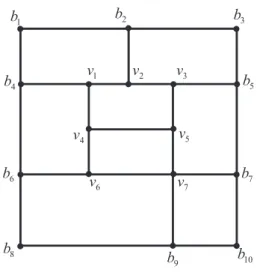
A T-mesh is basically a subdivision of some domain into rectangular cells that allow T-junctions (see Fig. 1). In this paper, only a rectangular domain is considered.
6 v 4 v 1 v v2 v3 5 v 7 v 1 b b2 b3 4 b 6 b 5 b 8 b 7 b 9 b b10
Let S (m, m′
,r, r′
)(T ) denote the space of functions of variables x, y that are piecewise polynomials of degree
m, m′and the class of smoothness Cr,r′
over the given T-mesh T . We also refer to S (m, m′
,r, r′)(T ) as the spline
space over T-mesh T .
In [2], the exact formula for the dimension of the space S (m, m′ ,r, r′)(T ) is obtained when m ≥ 2r + 1, m′≥2r′+ 1. In this case, dim S (m, m′ ,r, r′ )(T ) = (m + 1)(m′ + 1) f2− (m + 1)(r′+ 1) fh 1 −(m ′+ 1)(r + 1) fv 1+ (r + 1)(r′ + 1) f0, (1)
where f2is the number of cells of T , f1h and f1v
respec-tively are the numbers of horizontal and vertical interior edges (these intersect the interior of the rectangular do-main of T ), and f0 is the number of interior vertices
(these are in the interior of the rectangular domain). For instance, in Fig. 1, ν1, . . . , ν7 are interior vertices;
b2ν2, ν1ν4, vertical interior edges; and b4ν1, ν6ν7,
hori-zontal interior edges.
The method used to calculate the dimension of
S (m, m′
,r, r′)(T ) in [2] is based on B´ezier nets. In other
words, in [2], the formula for the number of elements in a minimal determining set of B´ezier ordinates is ob-tained.
Proofs of analogous results have been presented in [9] and [10] independently. However, the approach used in these studies is based on the smoothing cofactor method.
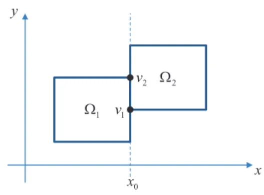
All these methods are based on the following simple observation. Let P1(x, y) and P2(x, y) be two
polynomi-als of degree m, m′defined on rectangular domains Ω 1
and Ω2, respectively, and having the common interval
(ν1, ν2) (see Fig. 2). Then, the piecewise polynomial
defined on Ω1S Ω2 has r-th order of smoothness for
variable x, if and only if
P1(x, y) − P2(x, y) = λ(x, y)(x − x0)r+1,
for some polynomial λ(x, y) of degree m − r − 1, m′for
variables x, y, respectively.
Here, we do not provide any detailed explanations of the approach used in these studies, but only mention the fact that the smoothing cofactor method appears to be the basic method for all further results concerning the dimension of a spline space over a T-mesh.
Thus, when m ≥ 2r + 1, m′≥2r′+ 1, one can express
the dimension formula in simple topological quantities such as the number of cells, edges, and vertices. This fact implies that any small variation, saving the topol-ogy of T-mesh T , does not change the dimension of the spline space S (m, m′ ,r, r′)(T ). x y 1 : 2 : 1 v 2 v 0 x
Figure 2: Two adjacent cells.
We will show hereafter that the conditions m ≥ 2r +1,
m′≥2r′+ 1 are optimal by giving explicit cases where
m = 2 r, m′ = 2 r′or m = 2 r − 1, m′ = 2 r′−1 for
which the dimension of the spline space changes with the position of the vertices.
In [10], Li et al. made the following improvement to the dimension formula. They found the constraint on the T-mesh that guarantees the dimension of the cor-responding spline space to be calculated using formula (1).
It appears that the last progress in the analysis of the dimension of a spline space, in a general case, was made in [11]. In this study, the results presented in [9] and [10] were reproved. In addition to the smoothing cofac-tor method, [11] exploited homology techniques to pro-vide additional insight on the analysis of the dimension of the spline spaces. Finally, the dimension of a space
S (m, m′,r, r′)(T ) is represented in this study in the
fol-lowing manner: dim S (m, m′ ,r, r′ )(T ) = (m + 1)(m′ + 1) f2− (m + 1)(r′ + 1) f1h−(m′ + 1)(r + 1) f1v+ (r + 1)(r′ + 1) f0+ hr,r ′ m,m′(T ), (2)
where the meaning of the term hr,rm,m′′(T ) is described in the next section.
Recall that the hierarchical T-mesh is either the ini-tial square or is obtained from a hierarchical T-mesh by splitting a cell along a vertical or horizontal line. A valuable observation was made in [11] about the up-per estimation of the summand hr,rm,m′′(T ) for a hierarchi-cal T-mesh T . This estimation allows one to establish the constraint on a hierarchical T-mesh T for the sum-mand hr,rm,m′′(T ) to be zero, and this constraint, in some manner, generalizes the one obtained in [10]. There-fore, if a hierarchical T-mesh T satisfies the constraint 2
proposed in [11], then the dimension of a spline space
S (m, m′
,r, r′
)(T ) is given by (1).
In a general case, the formula for the dimension of a space S (m, m′
,r, r′)(T ) cannot be expressed using
only the simple topological characteristics of T , such as
f2,f1h,f1v, and f0.
Recently, Li and Chen [1] demonstrated that the di-mension of a space S (m, m, m − 1, m − 1)(T ) may also depend on the geometry of a T-mesh T .
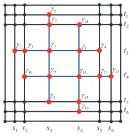
For instance, the dimension of a space S (3, 3, 2, 2)(T ) for T , shown in Fig. 3, depends on the values of the coordinates si,ti, i = 1 . . . 6. There are certain values
of the coordinates si,ti, i = 1 . . . 6 for which the
di-mension jumps with a small variation in these values; this indicates the instability in the dimension of space
S (3, 3, 2, 2)(T ).
The interesting question stated in [1] is how large the polynomial degree should be relative to the smooth-ness for the dimension of a spline space to be stable. In this work, we treat the new cases, S (4, 4, 2, 2)(T ) and S (5, 5, 3, 3)(T ), and provide certain examples of T-meshes T with instability in the dimension of the spline space. This shows that the constraints m ≥ 2 r + 1,
m′ ≥ 2 r′+ 1 known to yield a combinatorial
dimen-sion formula are optimal.
We note that the key approach to construct examples of T-meshes with instability in the dimension was in us-ing the abovementioned constraint on a T-mesh. The key was to violate this constraint to guarantee that the dimension is not given by (1). Unfortunately, the sum-mand hr,rm,m′′(T ) for some T-mesh T should be calculated as a rank of the corresponding matrix. However, it is dif-ficult to control even for small degrees m, m′. Therefore,
we specified coordinates of some nodes to simplify the calculations. As shown in the next section, the number of rows of this matrix linearly depends on the number of maximal interior segments. Therefore, to minimize the matrix size and make its rank unstable, we treated T-meshes with four maximal interior segments.
We investigated the cases S (4, 4, 2, 2)(T ) and
S (5, 5, 3, 3)(T ) because after the result of [1], they were
the first natural candidates to test the stability in the di-mension. The other motivation was that splines with small polynomial degree could be of interest in many applications.
We also assume that further generalizations of our re-sults require more sophisticated techniques. We believe that investigating the instability in the dimension of a space S (m, m′
,r, r′)(T ) is an important issue because it
provides a better understanding of the main problem, namely, how the basis of a space S (m, m′
,r, r′)(T ) can
be described.
The remainder of this work is organized as follows. In section 2, we explain the dimension formula (2) in detail and interpret it in a form pertinent for show-ing the instability in the dimension. In section 3, we explain how the dimension formula (2) can be used to prove the instability in the dimension of a spline space S (3, 3, 2, 2)(T ) for certain types of T-meshes T described in [1]. In section 4, we describe certain types of T-meshes T and prove the instability in the dimension of spline spaces S (5, 5, 3, 3)(T ) and S (4, 4, 2, 2)(T ). In section 5, we present the conclusions of this work and discuss future works.
2. Dimension of a spline space S(m,m′
,r,r′)(T) over T-mesh T: General formula
In this section, we explain the dimension formula (2) in detail. We also transform it into a form pertinent for showing the instability in the dimension. For reference, one can also find similar types of formulas for the di-mension of a spline space in previous works [9],[10].
The general formula (2) for the dimension of the space S (m, m′
,r, r′)(T ) for some T-mesh T of the
rectan-gular domain is found by using the homology technique [11].
The summand hr,rm,m′′(T ) in (2) may be considered as the dimension of the factor space M K [11]. The space
M is the direct sum M = M
ρ∈MIS (T )
[ρ]R(m,m′)−δ(ρ)
over the entire set of maximal interior segments
MIS (T ).
The maximal interior segment is the maximal union of connected edges of the same direction, such that there is no intersection with the border of the domain (for ex-ample, the segments ν1ν6and ν4ν5are all maximal
inte-rior segments of the T-mesh shown in Fig. 1).
Here, R(m,m′)denotes the space of polynomials of de-gree m, m′ of variables x, y, respectively, and δ(ρ) =
(0, r′ + 1) if ρ is the horizontal segment and δ(ρ) =
(r + 1, 0) if ρ is the vertical segment.
One can consider the space M as simply a vector space formed by the formal sums Σρ∈MIS (T )βρ[ρ], where
βρ ∈ R(m,m′−r′−1)if ρ is the horizontal maximal interior segment, and βρ∈R(m−r−1,m′)if ρ is the vertical maximal interior segment.
The subspace K ⊂ M has the following form:
K = Σγ∈T0 0(∆ r,r′ h [ρv(γ)] − ∆ r,r′ v [ρh(γ)])R(m−r−1,m′−r′−1),
where T00is the set of vertices of maximal interior seg-ments (for instance ν1, ν4, ν5, and ν6are all points of T00
for the T-mesh shown in Fig. 1). In addition,
∆r,rh ′= (y − yγ)r
′+1
, ∆r,rv ′= (x − xγ)r+1,
where xγ,yγ denotes the x, y coordinates of the vertex
γ. Furthermore, ρh(γ) and ρv(γ) are the corresponding
horizontal and vertical maximal interior segments con-taining the vertex γ (for example, in Fig. 1, ρh(ν4) =
ν4ν5, ρv(ν4) = ν1ν6). For more details, see [11].
To investigate the question of instability in the dimen-sion of a space S (m, m′,r, r′)(T ) over some T-mesh T , it
is only necessary to consider the summand hr,rm,m′′(T ). Let n be the number of vertices of T0
0, and lh,lvbe
the numbers of horizontal and vertical maximal interior segments, respectively. One can interpret hr,rm,m′′(T ) for some T-mesh T in terms of the rank of the correspond-ing matrix. Indeed,
hr,rm,m′′= dimM − dimK = (m + 1)(m ′ −r′ )lh+ (m′ + 1)(m − r)lv−(m − r)(m′−r′)n+ dimN.
where N is the subset
N ⊂M
γ∈T0 0
R(m−r−1,m′−r′−1),
so that each element of N is a set of polynomials
D
αγ∈R(m−r−1,m′−r′−1), γ ∈T0
0
E ,
such that it satisfies the following conditions:
Σγ∈ρhαγ(x − xγ)
r+1= 0 (3)
for each horizontal maximal interior segment ρh, and
Σγ∈ρvαγ(y − yγ) r′+1
= 0 (4)
for each vertical maximal interior segment ρv.
However, the space N can be represented as the space of solutions of the system of linear equations Lv = 0, where v is the column vector of coefficients of polyno-mials αγ, γ ∈T00. Here, we do not describe the structure
of the matrix L in the general case because it is simpler to understand it from the examples below.
We simply note that the number of columns in matrix
L is (m − r)(m′−r′)n and the number of rows is (m +
1)(m′−r′)l
h+ (m′+ 1)(m − r)lv. One can compute dim N
as
dim N = (m − r)(m′−
r′
)n − rank L. Thus, for some T-mesh T,
hr,rm,m′′(T ) = (m + 1)(m′ −r′ )lh+ (m′ + 1)(m − r)lv−rank L. (5)
3. Example of T-mesh with instability in the dimen-sion of a spline space S(3,3,2,2)(T)
In order to establish the instability in the dimension of a spline space, it is necessary to find a T-mesh in which the dimension jumps for some small change in the mesh. The proof of dimension jumping is based on calculating the rank of the corresponding matrix L. For
m = m′,r = r′= m − 1, examples of such T-meshes are
found in [1].
We describe in detail the example given in [1] for the case m = m′= 3, r = r′= 2. 1
s
s
2s
3s
4s
6 1t
2t
3t
4t
6t
1 J 2 J 13 J 4 J 6 J 7 J 8 J 9 J 10 J J11 J12 5s
5 J 5t
3 J 14 J 15 J 16 JFigure 3: Unstable T-mesh for m = m′= 3, r = r′= 2.
For the T–mesh shown in Fig. 3, every element of the space N (see (3),(4)) is simply the 16-th dimensional column vector v of the real numbers αj,j = 1 . . . 16
(each αjcorresponds to the vertex γj, j = 1 . . . 16), such
that the following equations hold for arbitrary x and y:
Σ5i=1αi(x − xγi) 3= 0, Σ9i=5αi(y − yγi) 3= 0, Σ13i=9αi(x − xγi) 3= 0, Σ16i=13αi(y − yγi) 3 + α1(y − yγ1) 3 = 0.
Note that these equations correspond to the maximal in-terior segments γ2γ4, γ6γ8, γ10γ12, and γ14γ16,
respec-tively.
Because the coefficients of the polynomials in these equations are zero, one can obtain the following system of linear equations:
α2sk1+ α3sk2+ α5sk3+ α1sk4+ α4sk5 = 0,
α6t1k+ α7t2k+ α5tk3+ α9tk4+ α8tk5= 0,
α10sk2+ α9sk3+ α13sk4+ α11sk5+ α12sk6= 0,
α14tk2+ α1tk3+ α13tk4+ α15tk5+ α16t6k= 0,
for k = 0 . . . 3.
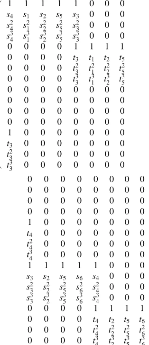
By writing these linear equations in the form Lv = 0, we obtain the following form for the 16 × 16 matrix L:
1 1 1 1 1 0 0 0 s4 s1 s2 s5 s3 0 0 0 s24 s21 s22 s25 s23 0 0 0 s34 s31 s32 s35 s33 0 0 0 0 0 0 0 1 1 1 1 0 0 0 0 t3 t1 t2 t5 0 0 0 0 t2 3 t 2 1 t 2 2 t 2 5 0 0 0 0 t3 3 t 3 1 t 3 2 t 3 5 0 0 0 0 0 0 0 0 0 0 0 0 0 0 0 0 0 0 0 0 0 0 0 0 0 0 0 0 0 0 0 0 1 0 0 0 0 0 0 0 t3 0 0 0 0 0 0 0 t2 3 0 0 0 0 0 0 0 t3 3 0 0 0 0 0 0 0 0 0 0 0 0 0 0 0 0 0 0 0 0 0 0 0 0 0 0 0 0 0 0 0 0 0 0 0 0 0 0 0 1 0 0 0 0 0 0 0 t4 0 0 0 0 0 0 0 t42 0 0 0 0 0 0 0 t3 4 0 0 0 0 0 0 0 1 1 1 1 1 0 0 0 s3 s2 s5 s6 s4 0 0 0 s2 3 s 2 2 s 2 5 s 2 6 s 2 4 0 0 0 s3 3 s 3 2 s 3 5 s 3 6 s 3 4 0 0 0 0 0 0 0 1 1 1 1 0 0 0 0 t4 t2 t5 t6 0 0 0 0 t24 t22 t25 t62 0 0 0 0 t34 t32 t35 t63
It is shown in [1] that the determinant of the matrix L is zero if and only if
(s3−s1)(s6−s4)
(t3−t1)(t6−t4)
=(s4−s1)(s6−s3)
(t4−t1)(t6−t3)
.
This equation holds, for instance, when si = ti, i =
1 . . . 6. However, a small change in coordinates si,ti, i =
1 . . . 6 makes the matrix L non-degenerate, which im-plies jumping of the rank(L), and therefore, because of (2) and (5) jumping of the dimension of the spline space. The bound of [11] yields in this case 0 ≤ h2,23,3(T ) ≤ 1.
Note that the structure of the T-meshes in [1] is not complicated, and these T-meshes only have four maxi-mal interior segments.
The observation of instability in the dimension of
S (m, m, m − 1, m − 1)(T ), given in [1], inspired us
to construct examples of T-meshes with instability in the dimension for the cases S (4, 4, 2, 2)(T ) and
S (5, 5, 3, 3)(T ).
4. Examples of T-meshes with instability in the dimension of spline spaces S(4,4,2,2)(T) and
S(5,5,3,3)(T)
In this section, we describe certain types of T-meshes
T and prove the instability in the dimension of spline
spaces S (4, 4, 2, 2)(T ) and S (5, 5, 3, 3)(T ).
We start with the case S (5, 5, 3, 3)(T ), because for the example of the T-mesh given for S (2, 2, 1, 1)(T ) [1], in-stability in the dimension of the space S (5, 5, 3, 3)(T ) has been demonstrated. This T-mesh is shown in Fig. 4.
4.1. Case: m = m′= 5, r = r′= 3 1
s
s
2s
3s
4s
5 1t
2t
3t
4t
5t
1 J 2 J 3 J 4 J J5 6 J J7 8 J 9 J 10 J 11 J J12 J J J J J J J J J JFigure 4: Unstable T-mesh for cases m = m′ = 5, r = r′ = 3 and
m = m′= 2, r = r′= 1. The polynomials αγi ∈R(1,1), γi∈T 0 0,i = 1 . . . 12 can be represented as αγi = k1i(x − xγi)(y − yγi) + k2i(x − xγi) +k3i(y − yγi) + k4i.
Let v denote the column vector of the length 48, such that for j = 4 l + r, r = j mod 4, the j-th coordinate of
v equals k(r+1)(l+1). Then, the set of polynomials
D
αγi,i = 1 . . . 12
is in N (see (3) and (4)) if and only if the following polynomials are zero:
Σγi∈ρk1i(x − xγi) 5+ k 3i(x − xγi) 4= 0, Σγi∈ρk2i(x − xγi) 5+ k 4i(x − xγi) 4= 0 (6)
if ρ is the maximal horizontal interior segment, and
Σγi∈ρk1i(y − yγi) 5+ k 2i(y − yγi) 4 = 0, Σγi∈ρk3i(y − yγi) 5+ k 4i(y − yγi) 4= 0 (7)
if ρ is the maximal vertical interior segment.
Let Vtdenote, for some given t, the rectangular 12 ×4
matrix of the form
Vt= 1 0 0 0 t −1 5 0 0 t2 −2 5t 0 0 t3 −3 5t 2 0 0 t4 −4 5t 3 0 0 t5 −t4 0 0 0 0 1 0 0 0 t −1 5 0 0 t2 −2 5t 0 0 t3 −3 5t 2 0 0 t4 −4 5t 3 0 0 t5 −t4 ,
and Hsbe a matrix of the form
Hs= 1 0 0 0 s 0 −1 5 0 s2 0 −2 5s 0 s3 0 −3 5s 2 0 s4 0 −4 5s 3 0 s5 0 −s4 0 0 1 0 0 0 s 0 −1 5 0 s2 0 −2 5s 0 s3 0 −3 5s 2 0 s4 0 −4 5s 3 0 s5 0 −s4 .
Then, from equations (6) and (7), one can obtain the system of linear equations for coefficients kji, j =
1 . . . 4, and i = 1 . . . 12 in the following manner:
Σγi∈ρHxγi k1i k2i k3i k4i = 0 (8)
if ρ is the maximal horizontal interior segment, and
Σγi∈ρVyγi k1i k2i k3i k4i = 0 (9)
if ρ is the maximal vertical interior segment.
We consider the system of linear equations (8) and (9) for coefficients kji, j = 1 . . . 4, and i = 1 . . . 12 in
terms of the linear system Lv = 0. Then, the matrix L has 4 × 12 = 48 columns and 12 × 4 = 48 rows. By using equations (8) and (9) and sequentially taking the maximal interior segments γ2γ3, γ5γ6, γ7γ9, and γ1γ11
(see Fig. 4), one can represent the matrix L in terms of 12 × 4 blocks Hxγi,Vyγi,i = 1 . . . 12 and zero blocks 0
filled with nulls in the following manner:
Vt3 Vt2 Vt5 Vt4 0 0 0 0 0 Hs4 Hs5 Hs2 0 0 0 0 0 0 Hs4 0 0 0 0 0 0 0 0 0 0 0 Hs3 0 0 0 0 0 Vt4 Vt2 Vt1 Vt3 0 0 0 0 0 Hs3 Hs1 Hs2
Thus, according to (5), for the given T-mesh, h3,35,5 equals 48 − rank (L).
In this work, we do not consider the question of cal-culating the rank of L for an arbitrary set of values
t1, . . . ,t5and s1, . . . ,s5to describe all possible positions
with instability in the dimension.
We are simply interested in the topology of the T-mesh and in providing some concrete values for
t1, . . . ,t5and s1, . . . ,s5such that dimension jumping
oc-curs for some small change in these values.
For instance, let us consider the following values:
t1= s1 = −2, t2= s2= −1, t3= s3 = 0,
s4= t4= 1, s5= t5= 2.
Then, rank L = 46. In order to be both rigorous and simple, we fix all values except t1and calculate the
de-terminant of the matrix L. One can check that the deter-minant is nonzero when t1 ,−2, implying that the rank
of L is equal to 48.
Therefore, the dimension of S (5, 5, 3, 3) is increased by 2 when t1 = −2, and therefore, we have dimension
jumping.
Notice that the bound of [11] yields 0 ≤ h3,35,5(T ) ≤ 4.
4.2. Case: m = m′
= 4, r = r′
= 2.
For S (4, 4, 2, 2)(T ), the example is a bit more curious. It is shown in Fig. 5.
The approach used in this subsection is the same as that used in the previous one.
1
s
s
2s
3s
4s
5 1t
3t
2t
4t
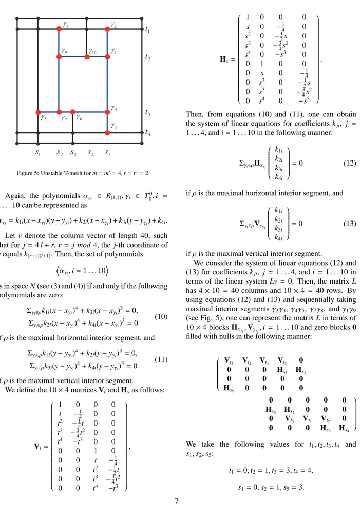
J J J J J J J J J J J J J1 2 J 3 J 4 J 5 J J7 J6 8 J 9 J J10Figure 5: Unstable T-mesh for m = m′
= 4, r = r′
= 2
Again, the polynomials αγi ∈ R(1,1), γi ∈ T
0 0,i =
1 . . . 10 can be represented as
αγi = k1i(x − xγi)(y − yγi) + k2i(x − xγi) + k3i(y − yγi) + k4i.
Let v denote the column vector of length 40, such that for j = 4 l + r, r = j mod 4, the j-th coordinate of
v equals k(r+1)(l+1). Then, the set of polynomials
D
αγi,i = 1 . . . 10
E
is in space N (see (3) and (4)) if and only if the following polynomials are zero:
Σγi∈ρk1i(x − xγi) 4+ k 3i(x − xγi) 3= 0, Σγi∈ρk2i(x − xγi) 4+ k 4i(x − xγi) 3= 0 (10)
if ρ is the maximal horizontal interior segment, and
Σγi∈ρk1i(y − yγi) 4+ k 2i(y − yγi) 3 = 0, Σγi∈ρk3i(y − yγi) 4+ k 4i(y − yγi) 3= 0 (11)
if ρ is the maximal vertical interior segment.
We define the 10 × 4 matrices Vtand Hsas follows:
Vt= 1 0 0 0 t −1 4 0 0 t2 −1 2t 0 0 t3 −3 4t 2 0 0 t4 −t3 0 0 0 0 1 0 0 0 t −1 4 0 0 t2 −1 2t 0 0 t3 −3 4t 2 0 0 t4 −t3 , Hs= 1 0 0 0 s 0 −1 4 0 s2 0 −1 2s 0 s3 0 −3 4s 2 0 s4 0 −s3 0 0 1 0 0 0 s 0 −1 4 0 s2 0 −1 2s 0 s3 0 −3 4s 2 0 s4 0 −s3 .
Then, from equations (10) and (11), one can obtain the system of linear equations for coefficients kji, j =
1 . . . 4, and i = 1 . . . 10 in the following manner:
Σγi∈ρHxγi k1i k2i k3i k4i = 0 (12)
if ρ is the maximal horizontal interior segment, and
Σγi∈ρVyγi k1i k2i k3i k4i = 0 (13)
if ρ is the maximal vertical interior segment.
We consider the system of linear equations (12) and (13) for coefficients kji, j = 1 . . . 4, and i = 1 . . . 10 in
terms of the linear system Lv = 0. Then, the matrix L has 4 × 10 = 40 columns and 10 × 4 = 40 rows. By using equations (12) and (13) and sequentially taking maximal interior segments γ2γ3, γ4γ5, γ7γ8, and γ1γ9
(see Fig. 5), one can represent the matrix L in terms of 10 × 4 blocks Hxγi,Vyγi,i = 1 . . . 10 and zero blocks 0
filled with nulls in the following manner:
Vt2 Vt1 Vt4 Vt3 0 0 0 0 Hs5 Hs1 0 0 0 0 0 Hs5 0 0 0 0 0 0 0 0 0 Hs3 Hs2 0 0 0 0 Vt3 Vt1 Vt2 0 0 0 0 Hs2 Hs4
We take the following values for t1,t2,t3,t4 and
s1,s2,s5:
t1= 0, t2= 1, t3= 3, t4= 4,
If we substitute s3 = s4, then the rank of L is 38,
otherwise it is 39. This means that the dimension of
S (4, 4, 2, 2) for the given T-mesh increases by 1 when s3 = s4. Again, the bound of [11] yields 0 ≤ h2,24,4(T ) ≤
4.
Note that both examples have only four maximal in-terior segments and their structures are quite simple.
5. Conclusions and future work
In this work, we proved the instability in the di-mension of a spline space S (m, m′
,r, r′
)(T ) over certain types of T-meshes T for the new cases m = m′= 4, r =
r′= 2 and m = m′= 5, r = r′= 3. The constructed
ex-amples have only four maximal interior segments and appear to be the simplest ones in some sense. One can construct more complicated examples of T-meshes with instability in the dimension by some combinations of the T-meshes shown in Figs. 4 and 5 for the cases
m = m′ = 5, r = r′ = 3 and m = m′ = 4, r = r′ = 2,
respectively.
To prove the instability in the dimension, we specified the values of the node coordinates of the T-mesh for the following two reasons. First, our main focus is on un-derstanding the topology of a T-mesh with instability in the dimension, and second, calculating the rank of the matrix L is simplified considerably. This work does not accurately analyze the algebraic conditions for the node coordinates for the dimension to be unstable. However, such an analysis could be carried out by implementing a row reduction procedure to calculate the rank of matrix
L.
In the future, the following problems would be in-teresting to explore. The first is the investigation of the instability in the dimension for the following, more gen-eral cases: m = m′
,r = r′
and 2r + 1 > m. The prob-lem is that the analysis of the rank of matrix L is non-trivial in more general cases; therefore, we might need to use another interpretation of the dimension formula. The second is the description of classes of T-meshes for the dimension of a space S (m, m′
,r, r′)(T ) to be
sta-ble and controlled by some topological characteristics. The work of [11] made progress in this regard, but we believe that it could be considerably strengthened by a more careful analysis of hr,rm,m′′. We intend to investigate these questions in our future work.
6. Acknowledgement
This research was supported by the National Re-search Foundation of Korea(NRF) grant funded by the
Korea government(MEST) (No. 2011-0018023) and partially supported by the Industrial Strategic technol-ogy development program, 10035474, Development of inspection platform technology based on 3-dimensional X-ray images funded by the Ministry of Knowledge Economy(MKE, Korea).
References
[1] X. Li, F. Chen, On the instability in the dimension of splines spaces over T–meshes, Computer Aided Geometric Design 28 (2011) 420–426.
[2] J. Deng, F. Chen, Y. Feng, Dimension of spline spaces over T–meshes, Journal of Computational and Applied Mathematics 194 (2006) 267–283.
[3] J. Deng, F. Chen, X. Li, C. Hu, W. Tong, Z. Yang, Y. Feng, Poly-nomial splines over hierarchical T–meshes, Graphical models 74 (2008) 76–86.
[4] X. Li, J. Deng, F. Chen, Surface modeling with polynomial splines over hierarchical T–meshes, Visual Computer 23 (2007) 1027–1033.
[5] J. A. Cottrell, T. J. R. Hughes, Y. Bazilevs, Isogeometric Anal-ysis: Toward Integration of CAD and FEA, John Wiley & Sons, 2009.
[6] N. Nguyen-Thanh, H. Nguyen-Xuan, S. Bordas, T. Rabczuk, Isogeometric analysis using polynomial splines over hierar-chical T-meshes for two-dimensional elastic solids, Computer Methods in Applied Mechanics and Engineering 200 (2011) 1892–1908.
[7] A.-V. Vuong, C. Giannelli, B. J ¨uttler, B. Simeon, A hierarchical approach to adaptive local refinement in isogeometric analysis, Computer Methods in Applied Mechanics and Engineering 200 (2011) 3554–3567.
[8] X. Li, J. Deng, F. Chen, Polynomial splines over general T– meshes, The Visual Computer 26 (4) (2010) 277–286. [9] Z. Huang, J. Deng, Y. Feng, F. Chen, New proof of dimension
formula of spline spaces over T–meshes via smoothing cofac-tors, Journal of Computational Mathematics 24 (4) (2006) 501– 514.
[10] C.-J. Li, R.-H. Wang, F. Zhang, Improvement on the dimension of spline spaces on T–mesh, Journal of Information and Com-putational Science 3 (2) (2006) 235–244.
[11] B. Mourrain, On the dimension of spline spaces on pla-nar T–subdivisions, preprint, inria–00533187, available at http://arxiv.org/abs/1011.1752v1.