Experimental study of fluid structure interaction on fuel assemblies on the ICARE experimental facility

HAL Id: hal-02563566

https://hal.archives-ouvertes.fr/hal-02563566

Submitted on 11 May 2020

HAL is a multi-disciplinary open access

archive for the deposit and dissemination of sci-entific research documents, whether they are pub-lished or not. The documents may come from

L’archive ouverte pluridisciplinaire HAL, est destinée au dépôt et à la diffusion de documents scientifiques de niveau recherche, publiés ou non, émanant des établissements d’enseignement et de

Experimental study of fluid structure interaction on fuel

assemblies on the ICARE experimental facility

Roberto Capanna, Guillaume Ricciardi, Emmanuelle Sarrouy, Christophe Eloy

To cite this version:

Roberto Capanna, Guillaume Ricciardi, Emmanuelle Sarrouy, Christophe Eloy. Experimental study of fluid structure interaction on fuel assemblies on the ICARE experimental facility. Nuclear Engineering and Design, Elsevier, 2019, 352, pp.110146. �10.1016/j.nucengdes.2019.110146�. �hal-02563566�

Experimental study of fluid structure interaction on fuel assemblies

on the ICARE experimental facility

Roberto Capannaa,⇤, Guillaume Ricciardia_{, Emmanuelle Sarrouy}b_{, Christophe Eloy}c

a_{DEN/DTN/STCP/LTHC, CEA CADARACHE, 13108, Saint-Paul-Lez-Durance, France}

b_{Aix Marseille Univ, CNRS, Centrale Marseille, LMA, Marseille, France}

c_{Aix Marseille Univ, CNRS, Centrale Marseille, IRPHE, Marseille, France}

Abstract

Accurate knowledge of the mechanical behaviour of the reactor core is needed to estimate the e↵ects of a seismic excitation on a nuclear power plant. Experimental works are needed in order to validate models and to have a better understanding of involved phenomena. The fuel assemblies, in the reactor core, are subjected to an axial water flow which modifies their dynamical behaviour. In this framework a new experimental facility, ICARE, is designed in order to investigate fluid structure interaction phenomena on half scale fuel assemblies. The design of the ICARE experimental facility allows to emphasise the e↵ects of the coupling between di↵erent fuel assemblies due to the presence of the water flow. In this paper a brief review of previous experimental facilities is presented and the new ICARE experimental

facility is illustrated. ICARE facility consists in 4 half scale fuel assemblies (2⇥ 2 lattice)

in a vertical channel submitted to axial flow; one of the assemblies is excited by an hydraulic jack. The aim of this paper is to discuss the experimental results obtained during four experimental campaigns on the ICARE set-up. First, the mechanical behaviour of a single fuel assembly is analysed, and the e↵ect of di↵erent experimental parameters is assessed. Added mass, added damping and added sti↵ness e↵ects due to the water flow are estimated. Later, the coupling between di↵erent assemblies is investigated. The presence of the flow induces hydrodynamic e↵ects on non excited fuel assemblies, both on excitation direction and transversal one. Furthermore the increase of the water flow causes the increase of the coupling forces and gives rise to a static coupling between the assemblies.

Keywords: Fluid Structure Interaction, Fuel Assemblies, Coupling, Experimental, Seismic Excitation

1. Introduction

In case of a seismic excitation, the whole reactor core moves and contacts between fuel assemblies can happen. The drop of control rods needs to be guaranteed in order to control

⇤_{Corresponding author}

the reactivity and core cooling needs to be ensured even when spacer grids strike each other during seismic excitation of a Pressurized Water Reactors (PWR). A way to ensure these two criteria is to prevent the spacer grids from buckling. Thus, a good modelling of the dynamical behaviour of fuel assemblies is needed. In order to validate the models, experimental results are also needed. This paper will focus on the experimental part of fluid structure interactions on fuel assemblies.

A reactor core (PWR) is made of several fuel assemblies (between 150 and 250 depending on the power of the reactor). A PWR fuel assembly stands between four and five meters high, is about 20 cm across and weighs about 800 kg. Each fuel rod has a diameter of about 1 cm for 4 m height; the space between each fuel rod in the assembly is about 3 mm. Fuel rods are held together by grids (between 8 and 10 depending on the power of the reactor) distributed along the fuel assembly. Springs and dimples are used in between the grid and the rods in order to keep the fuel rods in position. The fuel assemblies are cooled down by an axial water flow (about 5 m/s). The presence of the water flow and the structure gives rise to complex phenomena of interaction between the fluid and the structure (Chen and Wamnsganss, 1972). The presence of the structure, in fact, influences the behaviour of the fluid, which itself influences the behaviour of the structure. We could outline two di↵erent sources of interactions, the first one due inertial forces and a second one due to viscous forces.

During the last decades several experimental facilities have been realised in order to study the fluid structure interaction phenomena involved in nuclear fuel assemblies. Since it would be complicated and very expensive to reproduce a scale one nuclear core, di↵erent facilities have been constructed during the years scaling some of the parameters (number of assemblies, size of assemblies, pressure, temperature, etc.). Hereafter a brief review of the previous experimental works is presented.

The first experimental tests were realised on a full scale PWR assembly under water flow in 1988. For the first time added mass and damping e↵ects due to the presence of water flow were observed and quantified (Tanaka et al., 1988; K., 1990).

Experimental tests were realised in 1990 on the EROS experimental facility. The facility,

made of 5 reduced scale (6⇥ 6 lattice) fuel assemblies on a shaking table, showed that the

assembly can be modelled as non-linear beam (Queval et al., 1991a,b).

Later, the test section ECHASSE was built in 1999. Two reduced scale fuel assemblies

(8⇥ 8) are put under a water axial flow. The experimental facility was built in order to

study impact forces between the assemblies and between assemblies and test section walls. Di↵erent experimental campaigns were realised, allowing to develop a model for the impact forces depending on the water flow rate (Collard and Vallory, 2001).

A few years later, a new experimental facility called CADIX was realised. For the first time the experimental facility was involving full scale fuel assemblies. The test section consisted in a row of six fuel assemblies in stagnant water (or air) put on a shaking table. CADIX has been used in order to study impact forces (Queval, 2001). The experimental results were used in order to validate numerical codes. E↵ects of confinement size were also investigated (Broc et al., 2001).

semblies passes through the realization of COUPLAGE, an experimental facility involving a three-dimensional arrangement of the fuel assemblies. COUPLAGE was made of 9 fuel

assemblies (3⇥3) in a highly reduced scale (4⇥4 lattice). The assemblies were held together

by only one spacer grid, placed in the middle. Only one of the 9 assemblies is excited by an hydraulic jack with a sinusoidal input. Even though the geometry of the experimental facil-ity is not representative of a nuclear reactor core, and the assemblies scale is too small to be able to well represent a real nuclear fuel assembly, the COUPLAGE experiments allowed to study coupling force between the fuel assemblies and to outline the presence of non negligible interaction forces between assemblies placed on di↵erent rows (Ricciardi et al., 2010). Since the facility is not well representative of reactor conditions, further experimental structures are required in order to better understand the involved phenomena.

In order to study the dynamical behaviour of real fuel assemblies another experimental facility using scale one fuel assemblies (made of depleted uranium) was constructed: HER-MES T. It has loop conditions lower than real operative conditions (55 bar and 50 C) but can host 2 scale one fuel assemblies. Furthermore, one of the two assemblies can be excited by an hydraulic jack, and the walls of the structure have transparent portholes allowing to perform laser velocimetry measurements. Experimental campaigns on this facility allowed to measure the sti↵ness and the damping coefficients in order to quantify the e↵ect of the water flow on the added mass, added sti↵ness and added damping and to analyse the fre-quency response of a real nuclear fuel assembly (Ricciardi and Boccaccio, 2014). Some laser measurements of the fluid velocity field were performed.

From this quick overview of the previous experimental works performed on the study of fluid structure interactions on fuel assemblies, we can conclude that the impact force between fuel assemblies have been widely investigated during the years on di↵erent scales. On the other hand, the coupling phenomena involving di↵erent fuel assemblies have only been investigated on a small experimental structure (COUPLAGE) using very simplified

fuel bundles (3 grids, 4⇥ 4 lattice) which are not representative of real fuel assemblies.

For these reasons a new experimental facility has been designed and constructed at CEA Cadarache: ICARE. The main objective of this experimental facility is to study the coupling between di↵erent fuel assemblies depending on the confinement size and on the flow velocity. The fuel assemblies are not of real size (half length), but they are well representative of real

fuel assemblies (5 grids and 8⇥ 8 lattice rods).

In this paper the main results coming from the experimental campaigns realised on the ICARE facility will be analysed. The paper is organised as follows: in the first section the experimental facility is illustrated, in the second part the experimental campaigns and data analysis tools are presented, then the experimental results are discussed and analysed. 2. ICARE Experimental Facility

The ICARE experimental facility has been recently realised at CEA. A global description of the facility will follow in this section as a matter of clarity for the understanding of experimental results.

Compensation Tank Heat Exchanger Pressure Sensors Temperature Sensors Centrifugal Pump Flowmeter Position Sensors LDV System Test Section Jack Assembly Confinement Support Bellow Force Sensor Patella Jack 3 4 1 2

Figure 1: Scheme of the ICARE Experimental Facility.

The ICARE experimental facility is made of a closed water loop powered by a centrifugal pump, the test section, a compensation tank and an heat exchanger. The test section is

placed in vertical position with a square section of 22.5 cm⇥ 22.5 cm and hosts up to 4 fuel

assemblies arranged in a 2_{⇥ 2 lattice. The fuel assemblies length is 2.57 m, about half of the}

real fuel assemblies. Each of them is constituted of a squared lattice of 8_{⇥ 8 rods, in which}

there are 60 rods simulating fuel rods made of stainless steel or poly-methyl-methacrylate (PMMA) and 4 stainless steel guide tubes. The guide tubes are empty inside, and they are welded to 5 metallic spacer grids along the length of the assembly. The guide tubes have a structural function since they give rigidity to the assembly and they hold together fuel

rods. Each assembly has a section of 10.1_{⇥ 10.1 cm}2_{, and the 64 rods constituting it have}

a diameter of 9 mm with a pin pitch P/D = 1.33 (see left side of Figure 1). The top and bottom of the assembly are rigidly fixed to the guide tubes, and they are fixed to the test section through the Lower Support Plate (LSP) and the Upper Support Plate (USP). A scheme of the whole experimental facility is represented in Figure 1.

An hydraulic jack allows to excite one of the four fuel assemblies. For these experiments the right assembly in front of the door is excited, but the hydraulic jack can be placed

Grid 5 Grid 1 Grid 4 Grid 3 Grid 2 LVDT 22 LVDT 19 LVDT 23 LVDT 24 LVDT 17 LVDT 18 LVDT 20 LVDT 21 LVDT 14 LVDT 11 LVDT 15 LVDT 16 LVDT 9 CDDV LVDT 12 LVDT 13 LVDT 6 LVDT 3 LVDT 7 LVDT 8 LVDT 1 LVDT 2 LVDT 4 LVDT 5 Stabilization Grid Bottom Core Plate Closing Door Position Sensor Alternative position for hydraulic jack

Hydraulic Jack Force Sensor

Upper Core Plate

Figure 2: Scheme of the displacement sensors on the ICARE test section.

through a screw, and a force sensor is installed in between the hydraulic jack and the stem.

The force sensor (SM-S by PM Instrumentation) has a range from 500 N up to 500 N

with an accuracy of 0.045% of the full scale, meaning an uncertainty of _{±0.225 N. The}

hydraulic actuator is also equipped of a position sensor (_{±10 mm range and ±0.03 mm}

uncertainty). The force sensor will allow to measure the applied force, but it is not used in order to control the hydraulic jack. The control system uses the position sensor since its precision is much higher than the one of the force sensor. The hydraulic jack can be attached to two di↵erent grids, grid number 3 and grid number 4 (Figure 2). The possibility to excite the assembly on the middle grid and on the upper grid allows to excite di↵erent natural modes. When the hydraulic jack is attached to the middle grid, only the even modes will be excited, while when it is attached to the upper grid both even and odd modes will be excited. For more informations on the experimental facility and its components the reader is referred to Capanna (2018).

The test section is equipped with 24 LVDT (Linear Variable Di↵erential Transformer) position sensors. The LVDT sensors (model D5/300AW by PHIMESURE) have a working

range of ±7.5 mm and an uncertainty of ±0.0225 mm (0.3% of full scale). The position

sensors are installed at the level of the 2nd, 3rd and 4th grid. The first and the last grids

are not instrumented since they are close to the support plate and they are supposed not to move. For each spacer grid there are two position sensors, one monitoring the displacement on the x-direction and the other one on the y-direction, as represented in Figure 2. The CDDV sensor is the LVDT which is placed inside the hydraulic actuator. Furthermore, in

(a) Large confinement - 4 assemblies

(b) Small confinement - 4 assemblies

Slab 1

(c) Large confinement - 2 assemblies

Slab 3

(d) Small confinement - 2 assemblies

Figure 3: Possible configurations of the ICARE test section changing confinement size and number of assemblies.

order to measure the loop parameters, a temperature sensor and a static pressure sensor are installed at the inlet and outlet of the pump. In addition, a flow meter is installed on the loop, allowing to know the water flow rate circulating in the test section. The displacement sensors and the force sensor are collected with a sampling frequency of 2 kHz.

A specific characteristic of the ICARE experimental facility is the modular design which allows to chose between two di↵erent confinement sizes. The large confinement configuration leaves a 8 mm gap between the fuel assemblies and the walls and between each fuel assembly; the small confinement leaves only a 4 mm gap. Furthermore, plastic slabs are available in order to substitute fuel assemblies and to create configurations with one, two or four fuel assemblies. This modular design gives rise to four di↵erent possible configurations of the test section, which are represented in Figure 3.

The fuel rods of the bundles are realised in PMMA. The rigidity of the PMMA allows to maximize the ratio between the fluid forces and the structural forces (fluid forces become easier to measure). Furthermore, PMMA fuel assemblies have a natural frequency which

fits the resonance frequency of real fuel assemblies (' 2 4 Hz) in water.

Finally, the walls of the test section have some transparent portholes on the front face and on the lateral faces allowing to perform local fluid velocity measurements using laser ve-locimetry techniques. The laser veve-locimetry techniques implemented on the ICARE facility are the LDV (Laser Doppler Velocimetry) and PIV (Particle Image Velocimetry). Laser ve-locimetry measurements will be not discussed in this paper and will be the object of further publications.

3. Experimental Campaigns and Analysis Tools

The ICARE facility has been used to run several experimental campaigns. In this section the experimental matrix is presented and all the parameters that can be changed during di↵erent experimental campaigns are explained. Later on, the tools used to analyse the huge amount of data collected during the experiments are explained.

Assembly 1 Assembly 4 Assembly 2 Assembly 3 Excitation Direction

Figure 4: Scheme of the assemblies in the test section with the respective identification numbers.

For the sake of clarity, a scheme of the four fuel assemblies present in the experimental test section is reported in Figure 4 with the numbers corresponding to each assembly. As a reminder, during all the experiments the excited fuel assembly is always the assembly 1, and the excitation direction is always the x-direction.

3.1. Experimental Matrix

Four di↵erent experimental campaigns were conducted on the ICARE facility. First two campaigns involve the use of a large confinement (8 mm), while two further campaigns use a reduced size confinement (4 mm). The change of the confinement size allows to evaluate the e↵ects of the water bypass in between the wall and the assembly on the dynamic behaviour of the fuel assemblies.

For both confinement sizes, two experimental campaigns are run, one with the four assemblies and one with only two fuel assemblies. The presence of 4 fuel assemblies (arranged in square lattice) gives the possibility to investigate the out of plane phenomena in the coupling between fuel assemblies.

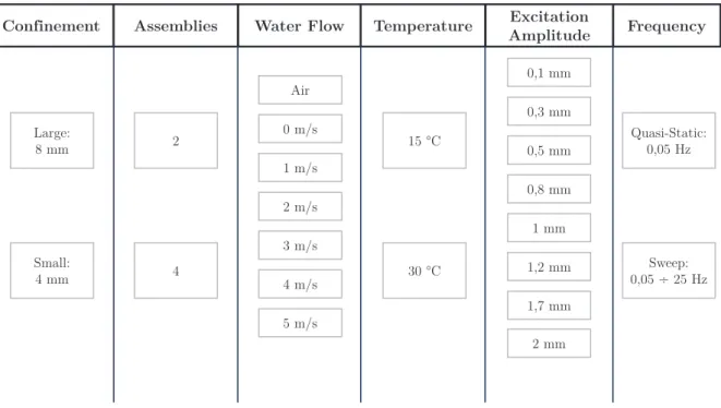
During all the four campaigns several experiments are run changing four di↵erent pa-rameters: the water flow velocity, the water temperature, the excitation amplitude and the excitation frequency (very low frequency sinus or swept sinus). The changes in the water flow velocity will allow to study the e↵ect of the water flow on the dynamics of the fuel assembly (added mass, added sti↵ness, added damping) and the e↵ects on the coupling be-tween di↵erent fuel assemblies. The range of water flow velocity goes from 0 m/s (stagnant water) up to 5 m/s. Experiments in air are also performed in order to know the nominal dynamical behaviour of the fuel assemblies. Experiments are repeated with two di↵erent water temperatures: 15 C and 30 C. Described flow conditions corresponds to Reynolds

investigate the e↵ect of the viscosity. In fact, even if the temperature di↵erence seems to be quite small, the viscosity changes more than 30%. Nevertheless, we realized that the tem-perature change introduce some non negligible changes in the properties of PMMA which should be taken into account in the analysis. The water temperature is not increased more than 30 C due to limitation on the PMMA of the fuel assemblies. The last parameter that was varied during the experiments is the excitation amplitude in a range from 0.1 mm to 2 mm. The change of the excitation amplitude can outline the presence of nonlinearities in the system.

Finally, two di↵erent kinds of excitation are given to the fuel assembly number 1. A first kind of excitation is a quasi-static excitation, consisting in a sinusoidal excitation with very low frequency: 0.05 Hz. With this excitation the dynamic behaviour does not play any role, but the hysteresis pattern of the fuel assembly is visible. The sti↵ness of the fuel assembly can also be calculated from the hysteresis plot, and the e↵ects of the water flow and confinement can be investigated.

The second type of excitation applied to the assembly aims to study the dynamics of the fuel assemblies. Thus higher frequencies are needed. The fuel assembly is excited from a frequency of 0.05 Hz to a frequency of 25 Hz with a swept sinus excitation. The excitation amplitude follows the Equation below:

a(t) = A sin ✓ ⇡(fmax fmin) Ts t2+ 2⇡fmint + 0 ◆ , (1)

where A is the excitation amplitude (from 0.1 mm to 2 mm), fmin = 0.05 Hz and fmax =

25 Hz are respectively the minimum excitation frequency and the maximum one and 0

indicate the phase at the origin (which is assumed to be 0 in all the experiments). The

quantity Ts represents the time needed to sweep from initial frequency to the final one. For

our experiments the sweep time used is Ts = 500 s thus giving a sweep velocity of 0.05 Hz/s.

Dealing with a swept sinus, the sweep velocity is an extremely important parameter. In fact, in order to catch the transfer function of a system, we need to excite each of the frequencies in an harmonic way. This is possible if the sweep velocity is small enough in order to avoid transient phenomena. For more details on such problems the reader is referred to Gloth and Sinapius (2004); Martert and Seidler (2001); Clement et al. (2014). The

international standard ISO 7626 defines the rules to respect for determining the transfer

function with a swept sinus excitation. For our experimental conditions, the sweep velocity of 0.05 Hz/s respects the rules defined in that document. An experimental verification of the sweep velocity has been performed by checking di↵erent sweep velocities.

Finally, the parameters which can be controlled in the di↵erent experimental campaigns are summed up in an experimental matrix in Figure 5.

3.2. Data Analysis Tools

This paragraph is devoted to the description of the analysis performed on the collected data during experimental campaigns.

Small: 4 mm Large: 8 mm 4 2 Air 30 °C 15 °C Sweep: 0,05 ÷ 25 Hz Quasi-Static: 0,05 Hz

Confinement Assemblies Water Flow Temperature _AmplitudeExcitation Frequency

0 m/s 1 m/s 2 m/s 3 m/s 4 m/s 5 m/s 0,1 mm 0,3 mm 0,5 mm 0,8 mm 1 mm 1,2 mm 1,7 mm 2 mm

Figure 5: Schematic representation of experimental matrix.

3.2.1. Quasi-Static Analysis

The first analyses are performed on the quasi-static data. The quasi static data are represented in a Force (exerted on the fuel assembly) VS Position (of the excited grid) plot where the hysteretic behaviour is outlined. The sti↵ness of the fuel assembly can be calculated from the slope of the curve. Plots for di↵erent amplitudes and di↵erent water flow velocities are compared.

3.2.2. Dynamic Analysis on the Excited Assembly

Later on, the data related to dynamic experiments are treated. First, the dynamic response of the excited assembly is analysed. Thus, the force data and position data of the excited grid are used. The transfer functions between the position and the force are calculated in order to outline the dynamical behaviour of the system (resonance frequencies, amplitude, damping, sti↵ness, etc.). Since the data are related to a swept sinus excitation, the transfer functions are calculated using the cross correlation product, and are defined as follows:

T FP F(f ) =

P (t) ? P (t)

P (t) ? F (t) , (2)

where T FP F(f ) is the transfer function in the frequency domain between position and force

P (t) ? F (t) is the spectral cross correlation between the position signal and the force signal. In addition, the coherence function is also analysed in order to understand if the transfer function calculated before is really due to external excitation imposed to the fuel assembly and is not due to noise or other phenomena. The coherence function is thus calculated as follows:

CohP F(f ) = | P (t) ? F (t) | · | P (t) ? F (t) |

| P (t) ? P (t) | · | F (t) ? F (t) | . (3)

Cross correlation functions are calculated using a windowing filter of Hamming type in order to clean up the noise from the signal. The transfer function are then used in order to evaluate the e↵ect of the di↵erent experimental parameters (as the flow velocity, temperature etc.) on the dynamic behaviour of the fuel assembly.

Furthermore, the transfer functions are used to perform an estimation of the dynamical

parameters of the fuel assembly as the modal mass (mi), the modal sti↵ness (ki) and the

modal damping (ci). The system is supposed to behave as a linear system, thus its transfer

function can be written as: T FP F(!) = 1 ki mi!2+ jci! = 1 mi(j2⇠i!i! (!2 !i2)) , (4)

where ! represents the circular frequency, ⇠i = ₂pc_mi

iki represents the damping ratio, !i =

p

ki/mi is the natural circular frequency. One can note that such a transfer function has its

maximum at the resonance pulsation !ri = !i

p

1 2 ⇠2

i. The theoretical transfer function

defined above is used to estimate the mass, sti↵ness and damping parameters of the fuel assembly with the use of the Least Square Method (LSM). Such a regression method for the estimation of the parameters is simple to implement but does not ensure the convergence to the good set of parameters for every initial guess. A trial and error routine is thus used in order to choose the proper initial guess allowing the LSM method to converge to the right values. Once the parameters estimated, the e↵ect of the water flow velocity and of the excitation amplitude is analysed.

3.2.3. Dynamic Analysis on the Coupling between Assemblies

The next step of the data analysis focuses on the study of the coupling between the excited assembly and the ones which are not excited. For experiments run with a water flow we expect that once the first fuel assembly is excited, an excitation is also induced on the other fuel assemblies due to the presence of the fluid. First, the coupling e↵ects on the Assembly 2 are analysed. Since the Assembly 2 is the one in the same direction as the excitation we expect to have the most important e↵ect of the coupling on this fuel assembly. Later, the couplings existing between Assembly 1 and other assemblies are also investigated. The coupling phenomena are investigated by using the mathematical tools already de-scribed in the previous sections. Transfer and coherence functions are calculated and the e↵ect of the di↵erent experimental parameters are investigated by comparison.

4. Experimental Results Analysis

In this section the experimental results obtained from the 4 di↵erent campaigns on the experimental facility ICARE will be discussed.

After a brief quasi-static analysis, data related to the dynamic behaviour of the excited fuel assembly are analysed first. Later, the coupling e↵ects between the excited fuel assembly and the other ones are addressed.

4.1. Quasi-Static Analysis

This paragraph aims to study the impact of di↵erent parameters (as water flow rate, excitation amplitude, etc.) on the quasi-static measurements. Since the main features of such a study are similar when changing the number of fuel assemblies and the confinement size, the most general condition with 2 fuel assemblies and large confinement is studied unless otherwise specified.

0 4 2 2 4 5 3 1 1 3 5 0 40 20 20 40 Force [N] 1m/s_1mm_15°C 1m/s_2mm_15°C 1m/s_3mm_15°C 1m/s_4mm_15°C

(a) Water flow rate 1 m/s at 15 C

0 4 2 2 4 5 3 1 1 3 5 0 80 60 40 20 20 40 60 80 Displacement [mm] Force [N] Air_4mm_15°C 0m/s_4mm_15°C 2m/s_4mm_15°C 5m/s_4mm_15°C (b) Excitation amplitude 4 mm at 15 C 0 4 3 2 1 1 2 3 4 0 40 20 20 40 Displacement [mm] Force [N] 0m/s_3mm_15°C 3m/s_3mm_15°C 0m/s_3mm_30°C 3m/s_3mm_30°C

(c) Excitation amplitude 3 mm at 15 C and 30 C

Quasi-static experiments allow to put in evidence the relation between the displacement of the fuel assembly and the e↵ort which is needed in order to move it without taking into account the dynamic e↵ects (excitation frequency 0.05 Hz). Figure 6 shows the force-displacement (on the x direction) relationships for di↵erent experimental conditions for the excited assembly.

Figures 6a, 6b and 6c show a typical hysteresis pattern. The e↵ort required to move the fuel assembly in one direction is not the same when the same fuel assembly is moved in the opposite direction. This hysteresis is mainly due to the presence of the support grids, which have several springs and dimples to hold the rods introducing important friction forces. The hysteresis behaviour becomes more important as the excitation amplitude becomes larger (Figure 6a). Hysteresis is in fact a non linear behaviour which is amplified by large amplitude displacements.

The knowledge of the force displacement relationship allows to also know the sti↵ness of the structure. The sti↵ness is in fact given by the ratio between the force necessary to move the body and the displacement itself. Thus the sti↵ness of the fuel assembly results to be the slope of the curves in Figures 6a, 6b and 6c. The slope of these curves, thus the sti↵ness of the fuel assemblies, is a↵ected by the water flow rate. When the flow rate increases, the slope of the force displacement plot also increases, meaning that the flow induces an added sti↵ness on the fuel assembly (Figure 6b). This added sti↵ness phenomenon is already known in literature and confirmed by experiments (Ricciardi et al., 2009; Ricciardi, 2016, 2018). The increasing of the temperature water seems, on the other hand, to have an opposite e↵ect (Figure 6c).

In conclusion, the quasi-static analysis allowed with some simple and fast experiments to catch the behaviour of one of the main properties of a fuel assembly (the sti↵ness) and to outline the presence of non linearities on the experimental facility ICARE mainly due to the presence of the support grids.

4.2. Dynamic Analysis on Excited Assembly

This section is devoted to the analysis of the dynamical response of the excited fuel as-sembly in dynamic experiments. Dynamic tests are performed by exciting the fuel asas-sembly over a frequency range from 0 Hz up to 25 Hz. Response of the excited fuel assembly (force and position sensors) and of the not excited ones (only position sensors) are acquired at a sampling rate of 2000 Hz (to catch fast components). Collected data are treated by means of transfer functions and analysed in the Fourier space, as already mentioned in Section 3.2.2.

The transfer functions between displacement and force on the excited assembly give infor-mation about the dynamical behaviour of the structure. The peaks represent the resonance frequencies, the departure of the curve represents the inverse of the sti↵ness and the width and intensity of the resonance peaks represent the damping of the structure.

4.2.1. Excitation Amplitude E↵ects

Figure 7a shows the dynamic behaviour of the excited fuel assembly when the excitation amplitude changes (from 0.1 mm up to 2 mm). Three peaks are visible in the frequency range from 0 Hz to 25 Hz. Each peak indicates respectively the first, second and third natural mode. The second and third modes are only exited for small amplitude excitations in order to avoid the fuel assembly to strike with the walls of the structure.

If the system were linear, one would expect the transfer functions to be perfectly identical. The transfer functions appear to be considerably di↵erent with one another, especially when considering the peaks amplitudes. These di↵erences are other proofs of the non linearities present in the system. The damping of the system appears to decrease with the increase of the excitation amplitude (peaks become narrower and higher) and the sti↵ness decreases (peaks slightly move to lower frequencies). The resonance frequencies slightly decrease with the increasing of the excitation amplitude.

The most important parameters that should be noted from the “In Air” dynamical anal-ysis of the fuel assembly are resonance frequencies. Even if they depend on the excitation amplitude, the average value can be considered to be a reference value for resonance fre-quencies. The first resonance mode in air appears at about 7 Hz, while the second and third resonances appear respectively at about 13.5 Hz and 20 Hz.

4.2.2. Water Flow E↵ects

Later on, the dynamical behaviour of the fuel assembly under water (stagnant and flow-ing water) is analysed. Even when the fuel assemblies are subject to stagnant water or moderate axial water flow (Figures 7b,7c), non linearitiy plays an important role in shifting the resonance frequencies, damping and sti↵ness values. The presence of the water flow attenuates the e↵ect of non linearities and when the water flow increases up to 5 m/s the di↵erences almost disappear (see Figure 7d).

The intensity of the water flow rate does play a very important role on the definition of the dynamical behaviour of the fuel assembly. This result was expected, since the interaction between the fluid and structure strongly changes when the water flow velocity changes.

One of the most important and most evident e↵ects of the presence of the water in the test section is a strong shift of the resonance frequencies. The presence of water strongly reduces the frequencies at which resonances occur (see Figure 8). The first resonance frequency decreases from about 7 Hz to about 4 Hz, the second one goes from 13.5 Hz to 8.5 Hz and the third one decreases from 20 Hz to 13 Hz. The increase of the water flow rate causes a further decrease of the resonance frequencies and a strong increase of the damping. When the water flow velocity is larger than 3 m/s (red curve in Figure 8 and Figure 7d) the system appears to be overdamped and resonances are not even visible.

The sti↵ness of the system also increases with the increasing of the water flow rate. The faster the water flows around the fuel assembly the stronger the water will oppose to the movement of the assembly itself. This opposition to the motion of the fuel assembly results in the increasing of the sti↵ness of the assembly.

The e↵ect of the presence of the stagnant water respect to “In Air” conditions is to decrease the resonance frequency (up to 50%) due to a strong increase of the added mass coefficient. The added mass e↵ect is thus the most important one in the transition from

0 2 4 6 8 10 12 14 16 18 20 22 24 26 0 0.2 0.1 0.3 0.05 0.15 0.25 0.35 Frequency [Hz] Transfer function 0.1 mm 0.3 mm 0.5 mm 0.8 mm 1.2 mm 2 mm (a) Air 0 2 4 6 8 10 12 14 16 18 20 22 24 26 0 0.1 0.02 0.04 0.06 0.08 0.12 0.14 0.16 Frequency [Hz] Transfer function 0.1 mm 0.5 mm 0.8 mm 1.2 mm 2 mm (b) Stagnant water: 0 m/s 0 2 4 6 8 10 12 14 16 18 20 22 24 26 0 0.02 0.04 0.06 0.08 0.01 0.03 0.05 0.07 0.09 Frequency [Hz] Transfer function 0.1 mm 0.5 mm 0.8 mm 1.2 mm 2 mm

(c) Water flow rate: 2 m/s

0 2 4 6 8 10 12 14 16 18 20 22 24 26 0 0.02 0.04 0.06 0.01 0.03 0.05 0.07 Frequency [Hz] Transfer function 0.5 mm 1.2 mm 2 mm

(d) Water flow rate: 5 m/s

Figure 7: Displacement-Force transfer functions for assembly 1 in large confinement with two assemblies for di↵erent flow rates at 15 C: comparison between di↵erent excitation amplitudes.

“In Air” conditions to stagnant water. This result is known in literature (Brennen, 1982; Wendel, 1956).

4.2.3. Confinement and Assemblies Configuration E↵ects

The e↵ect of confinement size and the presence of two or four fuel assemblies is now analysed.

The confinement size determines the amount of water lying in the gap between the fuel assembly and the walls of the test section. It is thus supposed that this gap plays a role in the dynamic behaviour of the fuel assembly immersed in water (either stagnant or flowing water). Of course, the confinement size should not play any role in the dynamic behaviour of fuel assembly “In Air”.

Due to technical problems, when the confinement size of the test section was changed, the link between the hydraulic jack and the fuel assembly grid broke. The reparation of the same grid was not possible, thus the hydraulic jack was attached to the middle grid for

0 2 4 6 8 10 12 14 16 18 20 22 24 26 0 0.2 0.1 0.05 0.15 Frequency [Hz] Transfer function Air 0 m/s 1 m/s 2 m/s 5 m/s

Figure 8: Displacement-Force transfer functions for assembly 1 with 0.5 mm excitation amplitude in large confinement with two assemblies at 15 C: comparison between di↵erent water flow rates.

of large confinement experiments). If the system was linear, the dynamical behaviour of the system should not change when changing excitation location. The main di↵erence that one can expect is that when the fuel assembly is excited in the middle grid the even modes are not excited, but the odd resonance frequencies should not change. Since the system is already proven to be non linear, some e↵ect when changing excitation position are expected. The e↵ect of the confinement size changes are visible in Figure 9: the second resonance frequency is not visible for small confinements as expected. On the other hand, a remarkable shift on the resonance frequencies and on the departure amplitude of the transfer function (which corresponds to the inverse of the sti↵ness) is visible. The sti↵ness of the fuel assembly decreases and resonance frequencies are shifted when the confinement size changes. Anyway, this behaviour cannot be related exclusively to the confinement size changes, since the excitation point is changed.

The presence of 2 or 4 fuel assemblies does not a↵ect in a sensible way the dynamic behaviour of the excited fuel assembly both for large (solid lines in Figure 9) and small con-finement (dashed lines in Figure 9). Some di↵erences can be seen on the second vibration mode which seems to be attenuated when the 4 fuel assemblies are considered. This attenu-ation could be due to the flexibility of the fuel assemblies which are close to the excited one, which thus represent a moving boundary around the excited fuel assembly. Also, the water has more possibility to move transversally in the 4 fuel assembly configuration. Despite the small e↵ects of the number of assemblies on the dynamics of the excited assembly, it is useful to have the possibility to compare experimental tests with 2 and 4 fuel assemblies

0 2 4 6 8 10 12 14 16 18 20 22 24 26 0 0.1 0.02 0.04 0.06 0.08 0.12 Frequency [Hz]

Large Confinement 2 Assemblies Large Confinement 4 Assemblies Small Confinement 2 Assemblies Small Confinement 4 Assemblies

Figure 9: Displacement-Force transfer functions for di↵erent confinement sizes and di↵erent number of assemblies with an excitation amplitude of 1.2 mm at 15 C .

regarding the coupling e↵ects. One can expect, in fact, that the configuration with 4 fuel assemblies allows to study the coupling phenomena existing in the excitation plane and out of the excitation plane. This subject will be treated in Section 4.4.

4.2.4. Temperature E↵ects

The e↵ects of the water temperature are addressed by performing experiments at two di↵erent temperatures: 15 C and 30 C. The e↵ect of the viscosity changes can be thus analysed by comparing measurements at di↵erent temperatures.

The transfer functions of the excited fuel assembly appears to considerably increase (about 20%) in amplitude when the water temperature increases (see Figure 10). Further-more, the departure of the transfer function curve also increases of about 20%. In addition to that, the peaks translate to lower frequencies. When the water flow rate increases, the temperature e↵ects become less and less important.

These e↵ects are due to a decrease of the fuel assembly sti↵ness. It was thought that the observed phenomenon is a proof that the water temperature a↵ects the dynamic behaviour of a fuel assembly. As the temperature increases, the water viscosity decreases; the decrease of the water viscosity can change the added sti↵ness e↵ect.

Anyway, it was not expected that such a slight di↵erence in the water temperature can a↵ect the behaviour of the fuel assembly in such an important way. In addition, the parameter that was expected to be a↵ected the most was the apparent damping of the

0 2 4 6 8 10 12 14 16 18 20 22 24 26 0 0.1 0.02 0.04 0.06 0.08 0.12 0.14 Frequency [Hz] Transfer function 15°C 0 m/s 30°C 0 m/s 15°C 2 m/s 30°C 2 m/s 15°C 4 m/s 30°C 4 m/s

Figure 10: Displacement-Force transfer functions for 15 C VS 30 C at 1 mm excitation amplitude with two fuel assemblies in small confinement.

di↵erences reside in the changes of the constituting material properties. The PMMA, in fact, suddenly changes its Young’s modulus when the temperature increases of few degrees. The Young’s modulus rapidly decreases, inducing the whole sti↵ness of the assembly to decrease. In order to estimate the e↵ect of the Young’s modulus on the dynamic behaviour of the assembly one can recall the relationship:

fn/

r EI

m (5)

which indicates the proportionality between the Young’s modulus and the natural frequency of the beam. In order to estimate the changes of natural frequency due to a change in the Young’s modulus one should first determine the Young’s modulus of PMMA at the two temperature of interest: 15 C and 30 C. Few data are available in literature about the mechanical properties of PMMA and their dependence on the temperature. In the work of Abdel-Wahab et al. (2016) experiments are carried out in order to estimate PMMA properties at di↵erent temperatures. Values of PMMA Young’s modulus have been estimated at 20 C and 40 C to be respectively E(20 C) = 5140M P a and E(40 C) = 4088M P a. These data can be used to estimate by interpolation the Young’s modulus of PMMA at

15 C and 30 C which result to be E(15 C)⇡ 5400MP a and E(30 C) ⇡ 4600MP a. Thus,

the temperature change from 15 C to 30 C produce a change of the Young’s modulus of PMMA of about 15%. The change in the natural frequency can be thus estimated by using

the following equation:

✏fn = 1

p

1 ✏E (6)

which gives a change of the natural frequency of the beam of the order of 7%. This value can be compared with the experimental data of natural frequencies at 15 C and 30 C which can be extrapolated from Figure 10. The experimental change of natural frequency due to the temperature change is about 5%. One can thus conclude that in our experimental conditions, the changes of dynamical properties of fuel assemblies due to the temperature is mainly due to the changes of the mechanical properties of the PMMA (mainly Young’s modulus).

Experimental results thus prove that temperature a↵ects the dynamics of an excited fuel assembly due to a combined e↵ect of the viscosity reduction (and eventually density) and to the changes of material properties which reduce the sti↵ness of the structure. It is thus evident that from an experimental point of view it is important to control and stabilize the temperature of the water flow. ICARE facility is equipped with a refrigerated system

which is capable of controlling the water flow temperature in a very efficient way (_{⇠ 0.5 C}

accuracy).

4.3. Parameters Estimation

Previous discussion was based on the analysis of the transfer functions of the excited structure and some inference was done on the dynamic behaviour of the fuel assembly de-pending on the parameters. In particular, mass, sti↵ness, damping and resonance frequency have been cited. This paragraph aims to mathematically determine from the experimental data these dynamic properties of fuel assembly, which will allow us to completely describe the dynamics of the structure.

As described in Section 3.2.2 the analytical transfer function parameters are estimated from the experimental curves. For low damped systems the estimation method is pertinent and the estimated transfer function follows exactly the experimental curve with an error smaller than 2%. The implemented method is thus proved to be stable and to converge to the true solution when the water flow is lower than 3 m/s.

In Figure 11 the general behaviour of the main dynamic parameters of the excited fuel assembly are presented. Modal mass, damping, sti↵ness and resonance frequencies are iden-tified for the first three natural modes. With our instrumented fuel assembly which has sensors in three di↵erent vertical locations we are not able to identify higher modes than the third one.

The modal parameters of the assembly “In Air” are identified and they represent the reference values. First modal mass (Figure 11a) increases in a consistent way from “In Air” conditions to stagnant water (it becomes about three times larger). Then, when the flow rate increases it slightly decreases. This decreasing behaviour is also identified by Ricciardi (2016); Ricciardi and Boccaccio (2014) and seems to have an asymptotic behaviour. On the other hand, the third modal mass appears to continuously increase when the water flow rate increases. This behaviour is thought to be due to some errors in the parameters

0 −2 −1 1 2 3 4 5 6 0 20 40 60 10 30 50 70 Water Flow [m/s] Mass [Kg] 15°C − Mode 1 15°C − Mode 2 15°C − Mode 3

(a) Modal mass

0 −2 −1 1 2 3 4 5 6 20 10 2 4 6 8 12 14 16 18 Water Flow [m/s] Resonance Frequency [Hz] 15°C − Mode 1 15°C − Mode 2 15°C − Mode 3 (b) Resonance frequencies 0 −2 −1 1 2 3 4 5 6 0 0.2 0.4 0.6 0.1 0.3 0.5 Water Flow [m/s]

Reduced Damping Ratio

15°C − Mode 1 15°C − Mode 2 15°C − Mode 3

(c) Modal damping ratio

0 −2 −1 1 2 3 4 5 6 20 40 30 50 25 35 45 Water Flow [m/s] Stiffness [kN/m] 15°C − Mode 1 15°C − Mode 2 (d) Modal sti↵ness

Figure 11: Behaviour of the estimated dynamic parameters as function of the water flow rates for the first three modes with excitation amplitude 0.5 mm at 15 C with 2 assemblies in large confinement configuration.

Flow rate 1 m/s means “In Air”.

identification routine which lack in reliability for modes higher than the second one. The di↵erence between the modal mass of the fuel assembly immersed in water and the modal mass of the fuel assembly in air gives the added mass coefficient. Thus, the added mass coefficient for the first mode decreases with the water flow rate.

Resonance frequencies (Figure 11b) show the same behaviour for all the three modes: it suddenly decreases when passing from “In Air” condition to stagnant water, and then it continues to slightly decrease as the water flow rate increases. The big jump of the resonance frequency is mainly due to the modal mass jump (but also the sti↵ness a↵ects the resonance frequency).

The damping ratio (Figure 11c) shows a continuous and almost linear increasing trend as the water flow increases. The damping ratio changes in a very significant way: it doubles when passing from “In Air” condition to 2 m/s water flow.

The first modal sti↵ness (which is the most important contribution to the total sti↵ness) also increases (slightly) with the increase of the flow rate (Figure 11d). The e↵ect of the water

−1 −0.5 0 0.5 1 1.5 2 5 10 15 20 25 30 35 40 45 Water Flow [m/s] Mass [Kg] 0.5 mm 0.8 mm 1.2 mm 1.7 mm

(a) Modal mass

−1 −0.5 0 0.5 1 1.5 2 4 6 3 5 3.5 4.5 5.5 6.5 Water Flow [m/s] Resonance Frequency [Hz] 0.5mm 0.8mm 1.2mm 1.7mm (b) Resonance frequencies −1 −0.5 0 0.5 1 1.5 2 0.2 0.4 0.1 0.3 0.5 Water Flow [m/s]

Reduced Damping Ratio

0.5 mm 0.8 mm 1.2 mm 1.7 mm

(c) Modal damping ratio

−1.5 −1 −0.5 0 0.5 1 1.5 2 20 14 16 18 22 24 26 Water Flow [m/s] Stiffness [kN/m] 0.5 mm 0.8 mm 1.2 mm 1.7 mm (d) Modal sti↵ness

Figure 12: Behaviour of the estimated dynamic parameters as function of the water flow rates and excitation

amplitude for the first mode at 15 C with 2 assemblies in large confinement configuration. Flow rate 1 m/s

means “In Air”.

flow, increasing the sti↵ness of the assembly, was already outline by quasi-static analysis.

Sti↵ness coefficients for the third natural mode (order of magnitude of 102 _{kN/m) are not}

represented in Figure 11d for better visual results (out of scale).

Finally the e↵ects of non linearities appearing when changing the excitation amplitude can be quantified (see Figure 12). The modal parameters relative to the first mode are analysed and compared when the fuel assembly is excited with di↵erent amplitudes under di↵erent flow conditions. Either the modal mass, resonance frequency and modal damping appear to be a↵ected in a marginal way by the changes of the excitation amplitude. On the other hand, the modal sti↵ness is strongly a↵ected by the changes in the excitation amplitude (see Figure 12d). The sti↵ness coefficient appears to change more than 40% when the excitation amplitude changes from 0.5 mm to 1.7 mm. This important change is justified by the presence of the spring and dimples in the five support grids which hold the fuel rods.

−1 0 1 2 3 20 40 10 30 50 Water Flow [m/s] Mass [Kg] 15°C 30°C

(a) Modal mass

−1 0 1 2 3 20 30 15 25 35 Water Flow [m/s] Stiffness [kN/m] 15 °C 30 °C (b) Modal sti↵ness

Figure 13: Estimated modal sti↵ness and mass at 15 C and 30 C for the first mode with excitation amplitude of 0.8 mm with two assemblies in large confinement configuration.

in Figure 13. More in the specific, the mass coefficient (Figure 13a) increases when the temperature increases from 15 C to 30 C, but the trend for the two temperatures appears to be similar. On the other side, the sti↵ness coefficient shows a behaviour which changes in a consistent way when the temperature increases. The sti↵ness parameter, in fact has an asymptotic trend with respect to the water flow rate at 15 C, while it continues to increase (almost) linearly with the flow rate when the temperature is 30 C. The asymptotic behaviour of the sti↵ness coefficient is due to an equilibrium between inertial and viscous forces. When the temperature changes, the viscosity of water and the sti↵ness of PMMA change considerably, thus the equilibrium between viscous and inertial forces also changes. This result is confirmed by numerical calculations performed for calculating added sti↵ness e↵ects with di↵erent temperatures by Ricciardi (2016, 2018).

4.4. Coupling Between Di↵erent Fuel Assemblies

From the literature it is known that when a network of structures subject to an excitation is immersed in a liquid, the interaction between the fluid and the structure creates a coupling between the di↵erent structures which would otherwise behave independently (Pa¨ıdoussis, 1998, 2008; De Ridder et al., 2013, 2017).

In this section the coupling existing between the four di↵erent fuel assemblies of the ICARE experimental set up will be analysed. The results related to the small confinement configuration are discussed, but the same conclusions can be drawn for the large confinement configuration.

As a first approach, one can expect that the main coupling phenomenon will involve the excited fuel assembly (assembly 1) and the one which is in front of it (assembly 2) in the excitation direction (x direction). For this reason, the analysis of the coupling between fuel assemblies 1 and 2 (see Figure 4) is investigated first. The three di↵erent sensor locations are analysed (for sensor position see Figure 2). It is obvious that the fuel assembly is mostly excited in the top and bottom locations at the resonance frequency (only odd resonance

modes are excited), while for frequencies far from the resonance the most excited position is the central one (where the hydraulic jack is attached). The coupling intensity between the grids over the three di↵erent levels are similar.

0 2 4 6 8 1012 14 16 182022 24 26 0 0.1 0.02 0.04 0.06 0.08 0.12 0.14 0.16 Frequency [Hz] Transfer function

(a) Top grid over excited grid 0 2 4 6 8 1012 14 16 182022 24 26 0 0.2 0.1 0.05 0.15 Frequency [Hz] Transfer function

(b) Central grid over excited grid 0 2 4 6 8 1012 14 16 18 2022 24 26 0 0.1 0.02 0.04 0.06 0.08 0.12 0.14 0.16 Frequency [Hz] Transfer function

(c) Bottom grid over excited grid

Figure 14: Coupling transfer functions between excited grid of assembly 1 and grids of assembly 2 in the excitation direction for 0.5 mm excitation with 1 m/s water flow in 2 fuel assemblies small confinement configuration at 15 C. Measurements are showed for the three di↵erent levels.

In Figure 14 the ratios between the displacement of assembly 2 grids and the excited grid are presented in the frequency domain. The displayed curves can be read as a transfer function between the displacements of the two assemblies. The intensity of the coupling is stronger between the excited grid and middle grid of assembly 2 (Figure 14b), while it is about half of the intensity between the excited grid and top and bottom grids of assembly 2 (Figures 14a, 14c). A peak appears at about 8 Hz which corresponds to the second mode resonance frequency; even if this mode is not excited on the first assembly, it is excited on the second one due to the coupling.

4.4.1. E↵ects of Water Flow, Excitation Amplitude and Temperature on Coupling

In Figure 16a the coupling transfer functions between the central grids of Assembly 1 and Assembly 2 are represented for di↵erent water flow conditions. It is evident how the increasing of the water flow induces an increasing coupling between the two fuel assemblies at low frequencies. Anyway, by the analysis of the natural mode shape of the beam at its third natural mode one can deduce that the maximum couplings between the assemblies at the third mode will happen on the first and third grids.

The maximum induced displacement is about 25% of the displacement of the excited assembly for the stagnant water (third mode at the top and bottom levels) while it increases to 40% when the axial water flow rate is 4 m/s (see Figure 15). This demonstrates that an increase of the flow rate induces an increase of the coupling forces and that fluid structure interactions can induce the motion of a structure which is not in contact with the excited one. The high flexibility of the PMMA assemblies makes this phenomenon more accentuated that it really is in full scale fuel assemblies. As the water flow increases, a static coupling appears and the coupling becomes e↵ective on a wide range of frequencies. In addition an anti resonance peak appears at the frequency of 8.5 Hz which corresponds to the second

0 2 4 6 8 10 12 14 16 18 20 22 24 26 0 0.2 0.4 0.1 0.3 0.05 0.15 0.25 0.35 Frequency [Hz] Transfer function Water Flow: 0 m/s Water Flow: 2 m/s Water Flow: 4 m/s

Figure 15: Water flow e↵ects on coupling transfer functions between bottom grids of excited fuel assembly 1 and assembly 2 in the excitation direction for di↵erent water flow rates with 2 assemblies in small confinement configuration with an excitation amplitude of 0.5 mm.

natural frequency. When the flow increases, the coupling between bottom grids becomes more important, up to 40%.

Furthermore, by analysing the phase diagram of the transfer functions for di↵erent flow rates, one can outline how the increase of flow rate induces an important reduction of the phase lag all over the excited spectrum (see Figure 16b). The phase diagram give important informations about the nature of the coupling, since inertial coupling has no phase di↵erence, while viscous coupling has a ⇡/2 phase di↵erence. The experimental results proved thus that the increase of water flow rates induces an increase of the inertial fluid structure interaction forces.

The excitation amplitude does not a↵ect in a considerable way the intensity of coupling between the two fuel assemblies. Some small di↵erences are visible for low frequencies, but a clear trend cannot be identified.

The e↵ects of the temperature, on the other hand, are clearly visible (Figure 16c). The intensity of the coupling strongly decreases (about 25%) when the water temperature in-creases from 15 C to 30 C. The decrease of the coupling forces due to an increase of temperature is mainly due to the changes in the water viscosity. Viscous forces, in fact, plays an important role in the fluid structure interaction, and are also responsible for the propagations of the e↵orts in the water domain.

4.4.2. E↵ects of Assemblies Configuration on Coupling

The coupling between the two fuel assemblies can be a↵ected by the number of fuel assemblies in the test section and by the confinement size. In order to analyse the influence of these parameters on the coupling e↵ects Figure 17 resumes in a schematic way the magnitude

0 2 4 6 8 10 12 14 16 18 20 22 24 26 0 0.2 0.1 0.05 0.15 Frequency [Hz] Transfer function Water Flow: 0 m/s Water Flow: 2 m/s Water Flow: 4 m/s

(a) Water flow e↵ects at 15 C

0 2 4 6 8 10 12 14 16 18 20 22 24 26 Frequency [Hz] Phase [rad] Water Flow: 0 m/s Water Flow: 2 m/s Water Flow: 4 m/s

(b) Phase lag water flow e↵ects at 15 C

0 2 4 6 8 10 12 14 16 18 20 22 24 26 0 0.2 0.1 0.02 0.04 0.06 0.08 0.12 0.14 0.16 0.18 Frequency [Hz] Transfer function Water Flow: 1 m/s 15°C Water Flow: 1 m/s 30°C Water Flow: 2 m/s 15°C Water Flow: 2 m/s 30°C (c) Temperature e↵ects

Figure 16: Coupling transfer functions between central grids of excited fuel assembly 1 and assembly 2 in the excitation direction for di↵erent water flow rates and di↵erent temperatures with 2 assemblies in small confinement configuration with an excitation amplitude of 0.5 mm.

of the coupling e↵ects (in both x and y directions) between excited assembly and other ones at the first resonance mode for 2 and 4 assemblies, both in small and large confinement configurations. Observation made on these sets of experimental results obtained with the cited water flow rate and excitation amplitude are general, and can be extended to all the experiments performed.

It is demonstrated that the confinement size has a fundamental importance in the mag-nitude of the coupling phenomena. As expected, for small confinement, the magmag-nitude of coupling forces in the excitation direction are the double than for large confinement (blue arrows in Figures 17a and 17b). This phenomenon is mainly due to the distance between the assemblies which is very di↵erent between the two configurations. The presence of two or four fuel assemblies does not seem to perturb in a consistent way the coupling phenomena. The coupling between the two fuel assemblies can also happen on the direction orthogonal to the excitation direction, which are represented by black arrow in Figure 17. From a first

8 % 10 % _ExcitationExternal 2 % 11 % 100 % 9 % 5 %

(a) Four assemblies in large confinement

16 % 9 % 9 % 11 % 100 % 3 % 7 % External Excitation

(b) Four assemblies in small confinement

6 %

4 %

100 %

External Excitation

(c) Two assemblies in large confinement

14 %

3 %

100 %

External Excitation

(d) Two assemblies in small confinement

Figure 17: Coupling forces between excited grid of first assembly and corresponding grid of non excited assemblies for the first resonance mode for 0.5 mm excitation at 2 m/s water flows in all configurations at 15 C.

same order of magnitude that in the excitation direction for all the configurations and all the assemblies. Contrariwise, by a deeper analysis of the coherence functions one discovers that there is no coherence between the two signals. Thus the relation outlined by the transfer function is mainly noise, probably due to the axial flow which induces some vibrations on the fuel assemblies. Some experiments could be carried out to measure the induced vibrations on the assemblies only due to the flow itself, without external excitation. We can thus affirm that the out of plane coupling between assembly 1 and assembly 2 is negligible. There is, instead, evidence of an existing coupling in the excitation direction between the fuel assemblies 1 and 3 and 4. The intensity of these coupling forces strongly depends on the confinement size as can be seen by comparing blue arrows of assemblies 3 and 4 in Figures 17a and 17b.

5. Conclusions and Perspectives

This paper contributes to the experimental study of the vibrational behaviour of PWR fuel assemblies. The new experimental facility, ICARE, which allows to host four half scale

fuel assemblies has been described and experimental campaigns have been presented. Then their main results have been analysed and discussed in the context of seismic excitation.

The quasi-static analysis of the fuel assembly allowed us to analyse the non linearities of the system and to describe their e↵ects on the behaviour of the fuel assembly. The sti↵ness of the assembly can also be estimated from the slope of the quasi-static force-displacement relationship.

The dynamic analysis of the excited assembly allowed us to investigate the e↵ects of di↵erent experimental parameters on fluid structure interaction forces. The presence of the water flow induces a dramatic decrease of the resonance frequencies mainly due to an increase of the modal masses. As the water temperature increases, the sti↵ness of the assembly is reduced. This phenomenon is not only due to the changes in the water properties but it is also strongly a↵ected by the changes of the properties of the plastic materials the assembly is made of.

Furthermore, the quantities which characterise the dynamical behaviour of the fuel as-semblies (modal mass, modal damping, modal sti↵ness and resonance frequencies) have been estimated from the experimental transfer functions. Their estimation has proved to be ac-curate, allowing a quantitative analysis of their e↵ects. The added mass e↵ect appears to be the most important parameter, but added damping and added sti↵ness e↵ects cannot be neglected.

Finally, the displacement induced on the non excited fuel assemblies have been investi-gated. The presence of water (either stagnant or flowing) induces a hydrodynamic coupling between the di↵erent assemblies. This coupling induced a motion of the not excited as-semblies. The magnitude of the induced motion is used to estimate the magnitude of this coupling in the di↵erent directions. As expected, the most e↵ective coupling happens be-tween the excited assembly and the opposite one (assembly 2) in the same direction as the excitation. The coupling strongly depends on the water flow, and it increases as the flow velocity increases. The induced motion on the non excited fuel assemblies can reach val-ues above 40% of the externally imposed displacement. This analysis of the hydrodynamic coupling shows that the coupling increases with the flow velocity.

The experimental data collected during the experimental campaigns are not yet fully analysed. The LDV and PIV data will be exploited in relation to the coupling phenomena observed in this paper and will be the subject of further publications. In addition, these results will be compared with numerical results provided by a simplified model based on the potential flow theory in order to gain insight into the physical mechanisms causing the hydrodynamic coupling of fuel assemblies.

6. Acknowledgement

The authors are grateful for the financial support of the Electricit´e de France (EDF) and FRAMATOME.

References

Abdel-Wahab, A., Ataya, S., Silberschmidt, V., 2016. Temperature-dependent mechanical behaviour of PMMA: Experimental analysis and modelling. Polymer Testing .

Brennen, C., 1982. A review of added mass and fluid inertial forces. Technical Report Naval Civil Engineering Laboratory .

Broc, D., Queval, J., Rigadeau, J., Viallet, E., 2001. Analysis of confinement e↵ects for in water seismic tests on PWR fuel assemblies. SMiRT 16 .

Capanna, R., 2018. Modelling of fluid structure interaction by potential flow theory in a PWR under seismic excitation. PhD Thesis, Ecole Centrale Marseille .

Chen, S., Wamnsganss, M., 1972. Parallel-flow-induced vibration of fuel rods. Nuclear Engineering and Design .

Clement, S., Bellizzi, S., Cochelin, B., Ricciardi, G., 2014. Sliding window proper orthogonal decomposition : application to linear and nonlinear modal identification. Journal of Sound and Vibration .

Collard, B., Vallory, J., 2001. Impact forces on a core shroud of an excited PWR fuel assembly. ICONE 9 . De Ridder, J., Degroote, J., Van Tichelen, K., Vierendeels, J., 2013. Modal characteristic of a flexible

cylinder in turbulent axial flow from numerical simulations. Journal of Fluids and Structures .

De Ridder, J., Degroote, J., Van Tichelen, K., Vierendeels, J., 2017. Predicting modal characteristic of a cluster of cylinders in axial flow: from potential flow solutions to coupled CFD-CSM calculations. Journal of Fluids and Structures .

Gloth, G., Sinapius, M., 2004. Analysis of swept-sine runs during modal identification. Mechanical Systems and Signal Processing .

K., F., 1990. Flow-induced vibration and fluid-structure interaction in nuclear power plant components. Journal of Wind Engineering and Industrial Aerodynamics .

Martert, R., Seidler, M., 2001. Analytically based estimation technique for nonlinear dynamic problems. Internation Journal of Solids and Structures .

Pa¨ıdoussis, M.P., 1998. Fluid-structure interactions: slender structures and axial flow. Elsevier Academic Press.

Pa¨ıdoussis, M.P., 2008. Fluid-structure interactions: slender structures and axial flow. Elsevier Academic Press.

Queval, J., 2001. Seismic test of integrating full scale fuel assemblies on shaking table. SMIRT 16 . Queval, J., Gantebein, F., Rigadeau, J., 1991a. Experimental studies on seismic behaviour of PWR fuel

assemblies. SMIRT 11 .

Queval, J.C., Gantebein, D., Brochard, D., Rigadeau, J., 1991b. Seismic behavior of PWR fuel assemblies model and its validation. SMIRT 11 .

Ricciardi, G., 2016. Fluidstructure interaction modelling of a PWR fuel assembly subjected to axial flow. Journal of Fluids and Structures .

Ricciardi, G., 2018. Parametric study on confinement e↵ect on a fuel assembly dynamical behavior under axial flow. Journal of Fluids and Structures .

Ricciardi, G., Bellizzi, S., Collard, B., Cochelin, B., 2009. Modelling Pressurized Water Reactor cores in terms of porous media. Journal of Fluids and Structures .

Ricciardi, G., Bellizzi, S., Collard, B., Cochelin, B., 2010. Fluid-structure interaction in a 3 by 3 reduced scale fuel assembly. Science and Technology of Nuclear Installations .

Ricciardi, G., Boccaccio, E., 2014. Mass, sti↵ness, and damping identification for a pressurized water reactors fuel assembly by a proper orthogonal decomposition method. Journal of Pressure Vessel Technology . Tanaka, M., K., F., Hotta, A., Kono, N., 1988. Parallel flow-induced damping of PWR fuel assembly. ASME

PVP Conference Pittsburgh .