HAL Id: hal-00914021
https://hal-paris1.archives-ouvertes.fr/hal-00914021
Submitted on 4 Dec 2013
HAL is a multi-disciplinary open access
archive for the deposit and dissemination of
sci-entific research documents, whether they are
pub-lished or not. The documents may come from
teaching and research institutions in France or
abroad, or from public or private research centers.
L’archive ouverte pluridisciplinaire HAL, est
destinée au dépôt et à la diffusion de documents
scientifiques de niveau recherche, publiés ou non,
émanant des établissements d’enseignement et de
recherche français ou étrangers, des laboratoires
publics ou privés.
Recommendation Heuristics for Improving Product Line
Configuration Processes
Raúl Mazo, Cosmin Dumitrescu, Camille Salinesi, Daniel Diaz
To cite this version:
Raúl Mazo, Cosmin Dumitrescu, Camille Salinesi, Daniel Diaz. Recommendation Heuristics for
Im-proving Product Line Configuration Processes. Robillard M, Maalej W., Walker R. and Zimmermann
T. Recommendation Systems in Software Engineering, Springer, pp.100, 2014, 978-3-642-45135-5.
�hal-00914021�
Recommendation Heuristics for Improving
Product Line Configuration Processes
Ra´ul Mazo, Cosmin Dumitrescu, Camille Salinesi and Daniel Diaz
Abstract In mass customization industries, such as car manufacturing, configurators play an important role both to interact with customers and in engineering processes. This is particularly true when engineers rely on reuse of assets and product line en-gineering techniques. Theoretically, product line configuration should be guided by the product line model. However, in the industrial context, the configuration of prod-ucts from product line models is complex and error prone due to the large number of variables in the models. The configuration activity quickly becomes cumbersome due to the number of decisions needed to get a proper configuration, to the fact that they should be taken in pre-defined order, or the poor response time of configurators when decisions are not appropriate. This chapter presents a collection of recommen-dation heuristics to improve the interactivity of product line configuration so as to make it scalable to common engineering situations. We describe the principles, ben-efits and the implementation of each heuristic using constraint programming. The application and usability of the heuristics is demonstrated using a case study from the car industry.
Ra´ul Mazo
Universit´e Paris 1 Panth´eon-Sorbonne, 90 rue de Tolbiac, 75013 Paris - France, e-mail:Raul. [email protected]
Cosmin Dumitrescu
Universit´e Paris 1 Panth´eon-Sorbonne, 90 rue de Tolbiac, 75013 Paris - France, e-mail:Cosmin. [email protected]
Camille Salinesi
Universit´e Paris 1 Panth´eon-Sorbonne, 90 rue de Tolbiac, 75013 Paris - France, e-mail:Camille. [email protected]
Daniel Diaz
Universit´e Paris 1 Panth´eon-Sorbonne, 90 rue de Tolbiac, 75013 Paris - France, e-mail:Daniel. [email protected]
1.1 Introduction
Product Line Engineering (PLE) is a viable and important reuse based development paradigm that allows companies to realize improvements in time to market, cost, productivity, quality, and flexibility [8]. According to Clements & Northrop [9] PLE is different from single-system development with reuse in two aspects. First, devel-oping a family of products requires “choices and options” that are optimized from the beginning and not just a single product specification that evolves over time. Sec-ond, product lines imply a pre-planned reuse strategy that applies across the entire set of products rather than ad-hoc or opportunistic reuse. The product line strategy has been successfully used in many different industry sectors, and in particular, in software development companies [26], [9]. Many different kinds of artifacts can be reused: including requirements, to model fragments, code, test data. These artifacts can be embodied as patterns, libraries of classes and meta classes, services or param-eterized components. Reuse can be achieved in many different ways: instantiation, integration, composition or setting up parameters.
The product line (PL) is often so complex, that it is not even possible to make an extensive list of all possible products. One example is the vehicle product line of the French manufacturer Renault, which can lead to 1021 configurations for the
“Traf-fic” van product family [3]. On the one hand, in Internet applications, it is important to ensure short response times and support multiple users (e.g. the online Renault car configurator). On the other hand, engineering applications need to support the specification and configuration of large product line models. Due to their complexity and size, it becomes difficult for the engineer to parse and configure these models. This is where recommendation techniques can improve some of the shortcomings of product line configuration of large models. This chapter presents an application of recommendation heuristics to the configuration of product line models. It discusses the advantages of each of these heuristics in respect to experiments on a model of a family of parking brake systems.
In Section 1.2we present background information related to the configuration of product lines and variability modeling. This is also where introduce an industrial case, based on the configuration of an automotive electric parking brake (EPB) sys-tem. In Section1.3we introduce the set of heuristics for the configuration of product lines. In Section1.4we present a practical “hands-on” experience for transforming the product line OVM model to a GNU Prolog constraint model, followed by the im-plementation of heuristics in GNU Prolog. We continue with related work in respect to our approach on recommendation-based configuration of product lines, in Section 1.2.1. Finally, in Section1.5, we discuss the usage and advantages of each heuristic and explain the context where each of them should be applied, and conclude the chapter in Section1.6.
1.2 Background
PLE explicitly addresses reuse by differentiating between two kinds of develop-ment processes [26]: domain engineering and application engineering. The aim of the domain engineering process is to manage the reusable artifacts participating in the Product Line (PL) and the dependencies among them.
The reusable artifacts, called domain artifacts (e.g., requirements, architectural com-ponents, pieces of processes, methods, and tests) are related in a model representing the legal combinations of the reusable artifacts (called product line model). The aim of the application engineering process is to exploit the product line model in order to derive specific applications by reusing the domain artifacts. To generate new prod-ucts, PLE takes into account the customer requirements but also the constraints of the PL domain.
The specification of requirements in the context of PLs is called a configuration process. In PLE, a configuration process is a step-wise process, with the objective to deliver configurations that both satisfy the domain constraints, provided by the product line model, and the stakeholders’ requirements, which can be specified too [13]. Dealing with PL constraints in domain and application engineering has been the subject of extensive literature that suggests different approaches, mostly based on constraint andsatisfiability (SAT)problem solving [24], [28]. Configuration re-quirements can be completely specified (i.e., to have a complete configuration, oth-erwise called completely defined configurations in which all variables have a value) or partially specified (i.e., to have partial configuration, in other words, configura-tions in which some decisions remain to be achieved). Once a complete or a partial configuration is specified, it evolves in its own project with the aim to become a new product.
The main requirement of people using these models is to support the navigation of the large models. While some approaches suggest to handle the configuration pro-cess in advance, either in the PL specification itself [11], or in addition to it [1], recommendation is clearly a track that has been overlooked by the literature and that still needs to be considered.
In Chapter ??, Robillard et al. [27] introduce two categories of knowledge-based recommendation approaches: case-based recommendation [7] and constraint-based recommendation [32]. Broadly speaking, case-based recommendation treats recom-mendation as a similarity-assessment problem and constraint-based recommenda-tion as a process of constraint satisfacrecommenda-tion. In this chapter we consider a third cat-egory of knowledge-based recommendation which we call heuristics-based rec-ommendation. We classify this technique as a knowledge-based technique as it is based on a set of knowledge sources that were implemented as heuristics to recom-mend what element(s) to configure during product line model (PLM) configuration processes. There are no a priori limitations on how the heuristics presented in this chapter can be combined or the field in which they can be applied.
During the configuration process, is possible to make the distinction between three types of recommendation: recommendation based on the PLM, recommendation
based on a set of predefined heuristics and trace based recommendation:
• Recommendation based on the product line model: allows the user to perform choices according to his requirements, by navigating through the available alter-natives at any given moment. Most of the approaches in the product line literature deal with this type of recommendation by only taking into account explicitly de-fined information in the product line (variability) model.
• Heuristics-based recommendation: suggests choices that shorten the configura-tion time, leading to valid configuraconfigura-tions, based on a set of heuristics. The con-tribution of this chapter focuses on this type of recommendation.
• Trace-based recommendation: suggest choices based on previous (logged) con-figurations and the current stage and context of each project. This type of recom-mendation is out of the scope of this chapter.
1.2.1 Configuration of Product Line Models
An interactive product configurator is a tool that allows the user to specify a product according to his specific requirements and the constraints of the product line model to combine these needs. This process can be done interactively, i.e. in a step-wise fashion, and guided, i.e. proposing the resolution of certain requirements before others and automatically proposing a valid solution when there is only one possi-ble choice in the solution space. To be useful in the e-commerce context, a con-figurator must be complete (i.e., to ensure that no solutions are lost), allow order-independent selection/retraction of decisions, give short response times and offer recommendation to maximize the possibilities to have one satisfactory configura-tion. Solution techniques applied to the interactive configuration problem have been compared by Hadzic and Andersen [16] and Hadzic et al. [17]. They mainly dis-tinguish approaches based on propositional logic on the one hand and on constraint programming on the other hand. When using propositional logic based approaches, configuration problems are restricted to logic connectives and equality constraints [17,31]. Arithmetic expressions are excluded because of the underlying solution methods. These approaches have two steps. First, the feature model is translated into a propositional formula. In the second step the formula is solved by appropriate solvers, in particular SAT solvers [24], and BDD-based solvers [17,30]. BDD-based solvers translate the propositional formula into a compact representation, the BDD (Binary Decision Diagram). While many operations on BDDs can be implemented efficiently, the structure of the BDD is crucial as a bad variable ordering may result in exponential size and, thus, in memory blow up.
Feature models can be naturally mapped into constraint systems in order to rea-son (e.g., perform configuration) on them, in particular into CSPs as presented by Subbarayan [30], Benavides et al. [5], and Deursen and Klint [10]; into Constraint Programs over finite domains CPs as presented by Mazo et al. [20], and into Con-straint Logic Programs (CLPs) as presented by Mazo et al. [23].
There are several academic tools dealing with configuration of product line models (e.g., SPLOT, FaMa1, VariaMos [21], Feature Plug-in [2] but very few have looked at PL tools and their ability to answer industry needs [3].
Jiang et al. [18] propose a constraint-based recommendation technique that gives to stakeholders a minimal set of repair actions in situations where no solution can be found for their configuration choices. Their approach also takes into account the preferences of a customer community to include collaborative recommendation. Authors deal with the situation where no solution can be found for the customers’ configuration as a constraint satisfaction problem. Authors use a well-known collab-orative recommendation technique consisting in calculating the contribution of each configuration choice in terms of reliability, economy, and performance by means of a utility function (cf. Multi Attribute Utility Theory (MAUT) [34]). In that work the term utility denotes the degree of fit between a feature of the product and the given set of customer requirements.
1.2.2 Variability Modeling
In the automotive industry, reuse is a core asset that allows car manufacturers to develop products faster and stay competitive. One of the most promising ways to manage reuse is by means of a product line approach. In the PL approach, the valid combinations of reusable artifacts are represented by means of a product line model. There are several notations used in the industry to represent their product lines mod-els; for instance, the Orthogonal Variability Model (OVM) notation [26], the DO-PLER notation [11] and the constraint-based notations [3,22].
Since the industrial case used in this chapter is originality presented in the OVM notation, we will use this formalism to illustrate the application of the approach. OVM is a language to document variability though variants, variation points and variability dependencies among them.
The termvariantused in this chapter is specific to product lines, and is somewhat different from the same term used throughout the book. According to Pohl et al. [26], variants are associated to the different shapes of an artifact, available at the same time. The term is thus associated to variability in space of the product family artifacts, in opposition to variability in time, which according toPohl et al.is de-fined as “the existence of different versions of an artifact that are valid at different times” [26].
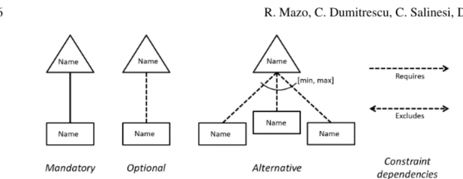
Figure1.1illustrates the concrete syntax of OVM. As the figure shows it, decision points are represented as triangles, and variants as rectangles attached to them. The figure also shows the five types of variability dependencies that can be used in OVM to specify how variants of a product line must or can be selected: mandatory, op-tional, alternative, requires, excludes.
Fig. 1.1: Legend of the OVM representation of variability
• A mandatory variability dependency between a variation point and a variant de-scribes that this variant must always be selected when the variation point is con-sidered for the configuration at hand.
• An optional variability dependency between a variation point and a variant de-scribes that this variant can be selected but does not need to be selected. • An alternative choice is a specialization of optional variability dependencies.
An alternative choice group comprises at least two variants which are related to a variation point by optional variability dependencies. The [min, max] bounds define that at least min and at most max variants can be selected for the product at hand.
• Additional dependencies between variation points and variants, e.g., to enforce that two variants of different variation points cannot be selected together.
1.2.3 Industrial Case
In this Section we will present our industrial case, from the automotive industry, that corresponds to the Electric Parking Brake (EPB) system by means of an OVM model, as well as some of the problems encountered in the traditional configuration strategy and observable on this particular model.
The orthogonal variability model enables the derivation of SysML models covering all system aspects from system requirements to physical implementation. The sys-tems engineering process requires that the engineering activities are performed in a certain order, enabling documentation, traceability of assets and providing deliver-ables at different project milestones. Our configuration strategy takes into account two common scenarios:
• Following the systems engineering analysis phases, with partial configurations for each phase. Each partial configuration has an impact on specific system model items [15]. The main concern is to follow the systems engineering approach, pro-viding partial models for document generation at each project milestone.
How-ever, a second concern is to minimize the number of steps to reach each valid partial configuration.
• Direct (quick) configuration of a system model. In this case the concern is to minimize the number of steps required to reach the valid desired configuration. In both of these cases, the traditional approach for an interactive configuration may present the following problems: a non-valid configuration can be reached as a result of the user sequence of choices, and the number of steps required to reach the con-figuration may not be minimal and require extra time and effort from the user. Furthermore, psychological studies [25] have shown that in a configuration process of complex products users do not exactly know their preferences when confronted with a set of alternatives, about which they do not possess solid previous knowl-edge. This may lead to delays for the exploration of alternatives at certain stages of the configuration process. It is particularly in this kind of situation that the approach presented in this chapter can useful. The OVM notation allows the variability of this industrial example to be represented with a concrete syntax that facilitates the un-derstanding and presentation of this case of a complex system. The Electric Parking Brake (EPB) system is a variation of the classical, purely mechanical, parking brake that ensures vehicle immobilization when the driver brings the vehicle to a full stop and leaves the vehicle. We have chosen this case because it satisfies the following requirements: (i) it represents an industrial case of reduced complexity; (ii) it does not pose confidentiality concerns; (iii) it contains enough variability for exploring our research questions. Figure1.2presents the main variations that were identified in the design of this system. The variability of the Electric Parking Brake system is explained according to the viewpoints specific to a systems engineering process: customer, context, design, internal behavior, and physical architecture.
• Customer visible variability corresponds to the variability stemming from the ve-hicle level by the product division.
The EPB proposes three types of service: Manual, Automatic and Assisted 2. The “manual” brake is controlled by the driver either through the classical lever or a switch. The “automatic” parking brake system variant may enable or disable the brake itself depending on the situation: for example when the driver turns off the engine and leaves the vehicle, the parking brake is activated. The “as-sisted” brake brings extra functions that aid the driver in other situations: such as assistance when starting the car on a slope. In all operational scenarios, except for the manual variant, the system can decide to lock the parking brake. This is for instance the case when the driver exits the car, the engine is stopped, and the vehicle starts on a slope. Thus the behavior of the system is given by the two vari-ation points: BrakeLock and BrakeRelease, where variants that involve automatic actions are mutually exclusive with the Manual type of parking brake. Hill start assistance is also a customer option, but the function can be allocated and im-plemented through different vehicle systems: through the electric parking brake
2The variability presented here does not necessarily use the same names and expose the same
itself (EPBEnabled variant) or through the classic braking system (ESCEnabled variant).
• The context viewpoint contains different facets of the system context, such as: system boundary variability, enabling systems and vehicle environment. In the EPB example, variants in the context refer to box type. The gear-box and the presence of certain types of trailers (VehicleTrailer variation point) have a direct impact on the internal behavior of the EPB system. The presence of a trailer, for example, may require the hill start assistance functionality to be disabled, or to adapt to the new total weight conditions.
• The design alternatives viewpoint specifies design decisions that impact the whole or parts of the technical solution.
The design decisions viewpoint includes: main solution alternatives (Architec-tureDesignAlternatives), choices on how to distribute the effort among the EPB and the main hydraulic braking system (ForceDistributionDesignAlternatives variation point), decision on software allocation to hardware (SoftwareAlloca-tionDesignAlternativesvariation point) and the allocation of the slope angle de-tection function (TiltAngleFunctionAllocation variation point). Allocation of this last function to a specific computer would obviously require that the computer (ECU) already exists.
• The variability entailed by the system internal behavior viewpoint impacts the states and transitions of the system physical and software components.
In the EPB , the braking strategy can vary depending on the deriving condi-tions. Each strategy requires specific information: Comfort and Dynamic require vehicle speed information (VSpeed) and the specific strategy for hill start assis-tance requires that there is a tilt angle sensor. Braking pressure is monitored after the vehicle has stopped for a certain amount of time (Temporary) for the single DC motor, puller cable solution, and permanently monitored (Permanent) for the other solutions
• The variability entailed by the physical architecture specifies variability in com-ponent decomposition, through optional or replaceable comcom-ponents, as well as physical interfaces variability between components.
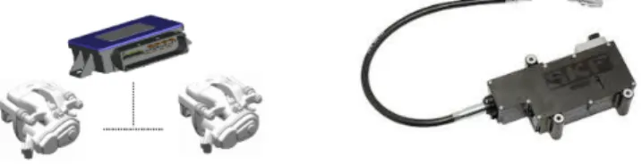
Physical variability of the EPB consists in the presence of different means of ap-plying the brake force: electric actuators mounted on the calipers or single DC motor and puller cable much like the traditional mechanical parking brake. Also the type of sensors available may vary depending on the configuration and needs. In addition to variation points and dependencies, variants attributes were associated to the different variants, in order to specify supplementary needed information re-garding the impact of PL configuration on performance (Braking Force Dissymme-try, Response Time on Brake), reuse (Vehicle Range Coverage) or cost increase in respect to a reference configuration of the system (Extra Engineering Cost). These attributes are numerical variables, that play a role during the derivation process and help the engineers make the right choices, by assessing the impact of their choices on the system configuration, and as the basis for supplementary constraints. Figure 1.3presents two examples of physical configurations of the EPB system. The instance on the right corresponds to a “puller cable” technical solution
(Archi-tectureDesignAlternatives - PullerCable), while the instance on the left corresponds to the solution based on “electric actuators” (ArchitectureDesignAlternatives - Elec-tricActuators). While system models can heavily rely on reuse for both of these configurations, only physical designs based on modular structures can further lever-age the reuse of components in different configurations on this level.
Fig. 1.3: Main design alternatives of the Electric Parking Brake system (PullerCable and ElectricActuator variants)
1.3 Recommendation Heuristics in the Product Line
Configuration Process
In an industrial context, letting the customers express their requirements that they want, while considering the constraints imposed by the product line model, entails a cumbersome and error prone configuration process. Evidence of these difficulties are multiple. For instance, in Business-to-Consumer commerce (B2C) in France, 60% of the shopping baskets in e-commerce are abandoned before purchase, be-cause the customer does not find a satisfactory configuration. The conversion rate visitor/buyer rarely exceeds 15%, according to FEVAD3. This difficulty is even more critical when the e-catalog contains a huge number of items, as is the case when the products to be sold are highly customized (e.g., computers or vehicles). One possible answer to this difficulty can be an interactive configuration process that recommends customers the best configuration alternatives to follow. When configu-ration is done interactively, the user specifies the characteristics of the product step-by-step according to his requirements, thus, gradually shrinking the search space of the configuration problem. This interactive configuration process is supported by a software tool (called configurator) that is intended to recommend to customers the best configuration alternatives that lead them to a satisfiable product in a minimum number of steps.
The main contributions of this chapter stands in a collection of heuristics that are in-tended to (a) help customers specify the characteristics of their products step-by-step
according to their requirements, and (b) to avoid useless or inefficient decisions. The collection of heuristics were designed to improve the configurators’ interactivity and thereafter successfully contribute to a faster and less error prone configuration pro-cess. A detailed description of the implementation of these heuristics is presented using Constraint Programming. This formalism was chosen because it can be im-plemented in a straight-forward way, and because it can be used to formalize any product line whatever notation was initially used to specify it [22,23]. The appli-cation of the heuristics is demonstrated using our Electric Parking Brake Systems case.
1.3.1 Principle of Heuristics-based Configuration
The objective of the application of heuristics to the configuration process is to in-crease the chance of success and to reduce the configuration time: (i) either by re-ducing the number of configuration steps, or (ii) by optimizing the computation time required by the solver to propagate configuration decisions.
Configuration is an interactive and iterative process. The user makes choices by assigning values to configuration variables. A step in the configuration process con-sists of a user choice and propagation of configuration decisions by the solver, if the value is valid, or of going back to the previous configuration state otherwise. Each value assignment can affect other variables. As a result, the order of value assignments has an impact on the overall number of steps of the process. Finally, the computation time of each configuration step is influenced by the complexity and size of the product line model.
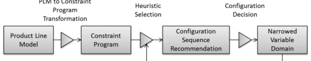
A generic configuration process iteration is presented in Figure1.4, as a flow of ac-tivities. Activities (e.g. selection, transformation, decision making) are represented as triangles, while assets, used in the configuration process (e.g. product line model, configuration sequence), are presented as rectangles. The asset may be the input of an activity, if it is on the left of that activity, or the produced output if it is placed on the right. Finally, the arrows link the graphical elements and point to the direction of the activity flow. Each configuration iteration consists in the following activities:
1. Product Line Model (PLM) transformation: The product line model, described using OVM, is transformed to a constraint program. We use the GNU Prolog language [12] to represent the constraint program and the GNU Prolog solver [12] as the engine to solve it. The configurator consists in a front-end (e.g., online interface) and a solver. The solver propagates the configuration decisions and ensures they are valid with regard to the product line model. The transformation from OVM to GNU Prolog, for the Electric Parking Brake case, is described in Subsection1.3.2.
2. Heuristic selection: The user can change the heuristics taken into consideration for future configuration steps, in respect to the desired objective. The appropriate context and advantages for each heuristic are discussed in Section1.5.
3. Variable prioritization: The configurator recommends variables to be configured, ordered in respect to the applied heuristics.
4. User choices: The user can follow the recommendations, or can continue to as-sign values to other variables of interest.
1.3.2 Representing Orthogonal Variability Models as Constraint
Programs
Alternative choices with cardinalities < m..n >, optional, mandatory, requires and excludes dependencies are represented as constraint programs as follows (further details are provided in [22]).
Alternative choices
An alternative choice is a dependency between a variation point and a collection of variants. Variation points are represented in constraint programming as Boolean variables and variants are represented as finite domain Integers. The semantic of this dependency can be represented by the following collection of GNU Prolog con-straints:
(Variant1> 0) <=> Bool Variant1,
(Varianti> 0) <=> Bool Varianti,
VariationPoint∗ m =< Bool Variant1+ . . . + Bool Varianti,
Bool Variant1+ . . . + Bool Varianti=< VariationPoint ∗ n
For instance, the < 1..1 > alternative choice of the variation point ParkingBrake-Serviceis represented in GNU Prolog as follows:
(PBSManual > 0) <=> Bool PBSManual, (PBSAutomatic > 0) <=> Bool PBSAutomatic, (PBSAssistance > 0) <=> Bool PBSAssistance,
ParkingBrakeService=
Optional dependencies
Optional dependencies relate variants and variation points in the following manner: (Variant > 0) ==> VariationPoint
For instance, the optional dependency between the variation point ClutchPedal and the variant ClutchPres is represented by the GNU Prolog constraint:
(ClutchPres > 0) ==> ClutchPedal Mandatory dependencies
Mandatory dependencies relate variants and variation points in the following man-ner:
(Variant > 0) <=> VariationPoint
For instance, VehicleWeight should be configured each time the father variation point (VehicleProperties) is configured in a product.The semantic of this dependency can be represented as follows in GNU Prolog:
(VehicleWeight > 0) <=> VehicleProperties Requires-type dependencies
Whether a Variant1requires a Variant2, the semantic of this kind of dependencies
can be represented by the following constraint :
(Variant1> 0) ==> (Variant2> 0).
Whether a VariationPoint1requires a VariationPoint2:
VariantPoint1==> VariationPoint2.
For instance, when the variant IntegratedDownsizedCalipers is selected in a config-uration, the variant ElectricActuator should also be selected. This can be represented as follows in GNU Prolog:
(IntegratedDownsizedCalipers > 0) ==> (ElectricActuator > 0) Excludes-type dependencies
Whether two variants (Variant1and Variant2) exclude each other, the semantic of
this kind of dependencies can be represented as follows: Variant1 ∗Variant2 = 0.
Whether two variations points (VariationPoint1and VariationPoint2) exclude each
other:
VariationPoint1* VariationPoint2= 0.
For instance, the fact that BLOnSystemDecision and PBSManual cannot be together in the same product is represented by the following constraint in GNU Prolog:
1.3.3 Configuration Heuristics
Configuration of variability models enables the realization of consistent system specifications from requirements at the domain level. However, as diversity plays a major role in automotive industry competitiveness, it is often difficult to manage the large number of variations that a vehicle system includes.
While users can express their priorities in a free configuration order, the configura-tor should choose the order that best optimizes its computational task and complete the configuration of the product line models based on the users decisions. The con-figurator completeness should ensure that no solutions are lost. Besides backtrack-freeness [16] should guarantee that the configurator only offers decision alternatives for which solutions remain, and the configurator should guarantee a short response time compatible with an interactive usage (e.g., with a web-based configuration). By defining a set of heuristics for product line configuration we intend to address the issue of decision ordering in order to allow the user to have access to pertinent choices and optimize the number of steps required to reach a complete configuration and the response time of the solver. The heuristics presented here are:
• Heuristic 1: Variables with the smallest domain first • Heuristic 2: The most constrained variables first • Heuristic 3: Variables appearing in most products first • Heuristic 4: Automatic completion when there is no choice
• Heuristic 5: Variables required by the latest configured variable first • Heuristic 6: Variables that split the problem space in two first
It is worth noting that there is not a predefined order to use the heuristics. Indeed, the configuration heuristics that can be suitable to be used in a configuration time t can be different from the configurations heuristics that the user will want to use at t+1. There are several heuristics that the user can select together for one or several configuration steps. In the case that users select several configuration heuristics, the configurator will propose a collection of candidate variables to configure accord-ing to the selected heuristics. For instance, if the users want to configure first the variables with the smallest domain (Heuristic 1) and the variables with the largest variability factor (Heuristic 3), the configurator will recommend them to configure the variables with the smallest domain decreasingly sorted by the variability factor. These heuristics are discussed below.
Heuristic 1: Variables with the smallest domain first
Principle: This heuristic recommends to choose first the variable with the smallest domain. The domain of a variable is the set of possible values that the variable can take according to its domain definition and the constraints in which the variable is involved. This strategy is known as “first fail principle” [6] and can be explained as “to succeed, try first where you are most likely to fail”.
Rationale:This could be counter-intuitive since configuring first the variable with the biggest domain reduce the search space the most. However, this decreases the possibility of obtaining a valid product at the end because that constrains the solver’s possibilities to choice a particular domain value that satisfies the set of constraints. Thus, even if setting first the variables with the largest domains reduces faster the solution space to be analyzed by the solver than setting first variables with small domains, it also decrease the possibility of having a valid product at the end of the configuration process. Of course, we prefer the latter choice. If all the variables have the same number of domain values (e.g., all variables are Boolean), the user can choose other heuristics to improve the configuration process.
Example: For instance, let us consider the variables:
V1= ForceDistributionDesignAlternatives, and
V2= ElectricalActionComponents.
They have enumeration domains with different cardinalities, where card(V1) >
card(V2), thus the second variable has the smaller. The choices associated to the first variable decide about the way brake force generation should be shared between the electric parking brake electrical actuators and the classic vehicle hydraulic sys-tem. The second variable decides about the physical architecture: single DC motor or two electric actuators attached to the vehicle calipers. The solver should propose variable ElectricalActionComponents first, according to the proposed heuristic. Advantages: This heuristic avoids unnecessary evaluations (e.g., when variable V2
is set to a particular value of its domain, the solver does not need to check for other values of V2) and increases the possibility to succeed the configuration process (i.e.,
configuring first the variables where the constraint program is most likely to fail, we increase the possibilities of the solver to succeed).
Heuristic 2: The most constrained variables first
Principle: Another heuristic, that can be applied when all variables have the same number of values, is to choose the variable that participates in the largest number of constraints (in the absence of more specific information on which constraints are likely to be difficult to satisfy, for instance). This heuristic follows also the principle of dealing with hard cases first.
Rationale: In industrial languages like the constraint networks [3] where there are no root artifacts to guide the configuration process, this heuristic allows identifying the variables that mostly reduce the number of choices in a configuration process. Example: In the EPB model, the PullerCable variant is one of the most constrained in this model, being linked to the way force is distributed among braking systems (ForceDistributionDesignAlternatives), internal system behavior (ForceMonitorO-nEngineStop) and physical implementation (DC motor). In consequence, it reduces other choices in the configuration process, directly linked to the initial variable. Advantages By setting first the variable related with the largest number of other variables the solver would automatically propagate the user’s choice to the largest
number of other variables. In that way the space of the solution is considerably re-duced after each choice, which reduces the number of configuration steps (user’s choices) and the average configuration time (solver’s inference time).
Heuristic 3: Variables appearing in most products first
Principle: This heuristic proposes configuring first the variables that have an im-pact on all potential products. To avoid the generation of all products of the PL, which is usually impossible in very large models [4,22], we propose two steps:(i) configure first the core variables, and (ii) configure the rest of variables once or-dered according to their impact on the solution space. To implement the first step, we use the computing the core elements operation fully automated in the VariaMos tool [21]. To avoid generation of all solutions in order to calculate the core elements as proposed by Schneeweiss et al. [29], we evaluate if each variable can take the nullValue(e.g., the 0 value on Boolean variables) in at least one correct configura-tion. If a variable cannot take its nullValue, the variable does not become part of the core variables of the product line model because this can never be omitted from any product. To know if a variable can take the nullValue in a valid configuration takes only few milliseconds even in the largest product line models available in literature; Details of this algorithm, its improvements, implementation and evaluation can be found in Mazo et al. [23]. The second step is implemented thanks to the operation of computing the variability factor of a given variable, and fully automated in our tool VariaMos [21]. This variability factor of a given variable corresponds to the ratio between the number of products in which the variable is present and the number of products represented in the product line model.
Rationale: The heuristic can be applied when the user needs to reach a valid con-figuration with as little input as possible. Fixing the values of the core variables (usually approximately 2/3 of the variables of the product line model [8]) decreases the size of the problem space in the same proportion, avoiding unnecessary input from the user. This also makes feasible the calculation of the variability factor of the remaining variables. The variables with a higher variability factor reduce the path to a valid product and the need for user input.
Example: In products where the customer requirements do not include assistance (ParkingBrakeService = Assistance) from the system, other than for parking brake situations, the option for hill start assistance and for disabling the hill start assistant function are excluded. In consequence, the definition of these variables does not ap-pear in all products, and according to this heuristic should not be proposed before core variables.
Advantages: This heuristic is useful because (i) it avoids wrong users’ configu-rations in the sense that core variables cannot be configured with nullValues, and (ii) the order proposed in this technique decreases the solver’s inference in finding satisfactory configurations.
Heuristic 4: Automatic completion when there is no choice
Principle: This heuristic provides a mechanism to automatically complete the con-figuration of variables where only one value of their domain is possible.
Rationale: Due to the fact that the aim is to eliminate, in the domains of variables yet to be instantiated, the values that are not consistent with the current instantia-tion, this heuristic also works when a variable has several values on its domain but only one is valid. This heuristic is automatically provided by most constraint solvers available on the market, with at least, three algorithms that implement it: Forward Checking, Partial Look-Ahead, Full Look-Ahead.
Example We consider variable V1= HillStartAssistance, V2= BrakeLock and V3=
ParkingBrakeService. Setting the value for V1= EPBEnabled, V2= OnSystemDecision
excludes all values for V3, except V3= Automatic, in which case this single possible
value should be selected automatically.
Advantage: The automatic assignment of values to variables, once there are no more alternative solutions, avoids the possibility of invalid configurations due to wrong values requested by the user. Therefore, it contributes to the success of the configuration process.
Heuristic 5: Variables required by the latest configured variable first
Principle: Another heuristic consists in choosing the variable that has the largest number of constraints with the past-configured variables.
Rationale: This heuristic has a particular application during configuration of en-gineering artifacts, where choices often represent enen-gineering decisions linked by causality relations. A choice may not be reached before a previous choice has been performed. In this particular context, following related variables (that serve for the reuse of engineering artifacts) would mean advancing in the design space towards a more detailed description of the system being configured.
Example: In the case of the EPB system we can find logical implications which have their origin in technical constraints or problem solving logic. For example, the system needs to be able to disable the hill start assistant function (HSADisable-Function), if a trailer is used (when the function is not able to adapt to the change of weight of the vehicle). In this case it is convenient to propose variable HSADis-ableFunctiononce variable VehicleTrailer = TrailerW 1 has been set, both for the user (logical flow of ideas), but also to avoid potential future conflicts in the config-uration.
Advantages: This heuristic allows conflicts to be identified as soon as possible (with regards to the number of configuration steps) in a configuration process. This hence, increases the possibility to fix the configuration conflicts and the possibility to suc-ceed in the configuration process.
Heuristic 6: Variables that split the problem space in two first
Principle: Breaking a problem into sub-problems is a powerful tool in many do-mains. This heuristic consists in setting first the variables splitting the problem space in two. Due to the fact that these variables have most potential to reduce the solution space, the application of this heuristic naturally reduces the number of configuration choices.
Rationale: This is due to the fact that after one choice, the solver will have a re-duced solution space to exam and the user will have fewer configurations to do. Several product line modeling languages (e.g., Feature models) are inspired by this principle and propose the use of a root element with two of more choices related by OR or XOR operators that divide the problem space in branches that can be easily removed from the solution space. To achieve this we need to search for variables that divide the problem space in roughly similar parts, searching the decision trees have almost the same depth for each of the values of the variable.
Example: In the case of the parking brake system, the choice concerning the pres-ence of the hill start assistance function splits the decision tree in roughly similar parts.
Advantages: Setting first the variables that break the problem in two equal parts, re-duces the computation time of future choices and increases the chances of reaching a completely defined product in a reduced number of steps.
1.4 Application to the Configuration of a Parking Brake System
One particular question that can be raised about the configuration heuristics that have been presented in this chapter is are they useful? Although only long-term ex-perience will provide a definitive answer to this question, one might be interested in looking for its implementation and its application in a real case. To do that, we have (i) implemented our collection of heuristics in the constraint logic programming solver GNU Prolog [12], and (ii) applied these heuristics in typical configuration processes of our industrial case. For each heuristic, we measure the time required by the solver to generate X products; then, we compare these results with the ones obtained when we do not use any heuristics or use a contra-sense approach in the same configuration process. The industrial case was developed in the broader con-text of introducing product line techniques in model based systems engineering [14]. Our Electric Parking Brake Systems (EPB) model (c.f. Figure1.2) is represented by means of the OVM notation [26] and is composed of 19 variation points, 46 variants, 16 alternative choices, 1 mandatory and 7 optional variability dependencies, and 28 additional dependencies (21 requires-type, 5 excludes-type, and 2 non-classified dependencies [22]). To present the feasibility of our approach and conclude what heuristics should be recommended for use during a product line configuration pro-cess, we first transform our EPB model into an automatically exploitable language, then we explain how to implement each heuristic and we compare the resultsgath-ered from their application to our industrial case.
Once our EPB model is represented as a GNU Prolog constraint program, we can apply our collection of heuristics to configure different Electric Parking Brake systems and measure the results obtained each time and compare them with the results obtained when no heuristic is used.
Heuristic 1: Variables with the smallest domain first
The GNU Prolog predicate f d labeling(Vars, Options) assigns a value to each vari-able of the list Vars according to the list of labeling options given by Options. Vars can be also a single finite domain variable. This predicate is re-executable on back-tracking. Options is an optional list of labeling options that specifies the heuristic to select the variable to enumerate. When no option is specified, the solver selects the leftmost variable in the list of variables (Vars) to enumerate in the configuration process.
This heuristic is already implemented in GNU Prolog solver and can be used in a configuration process by means of the following predicate:
f d labeling(Vars, [variable method( f f )]),
Where Vars is the list of variables of the constraint program (variation points and variants of our model) and variable method( f f ) is the GNU Prolog predicate of-fered by the solver to call the ff (first fail) heuristic in the current configuration process (i.e., in the current f d labeling).
Heuristic 2: The most constrained variables first
To implement Heuristics 2 in GNU Prolog we just need to sort the list of variables (Vars), where the first variables in the list are those that are more constrained, and then use the predicate f d labeling(Vars) in our configuration process. In our in-dustrial case, Vars = [PullerCable, ESPECU, PBSManual, ElectricActuator, Hill-StartAssistance, Static, TrailerW1, Permanent, DownsizedAndESPDynamicBrak-ing, VSpeed, HSADisableFunction, TraditionalPB, DCMotor, DownsizedAndEx-tratorqueESP, AuxiliaryBrakeRelease, EU, BROnSystemDecision, BROnSystemDe-cision, TiltSensorIn1, TiltSensorIn2, TrailerW2, EPBEnabled, Comfort, Calipser-WithIntegr, EActuator, PBSAssistance, FullEPB, Temporary, ClutchPres, Dedicat-edECU, Dynamic, BLOnSystemDecision, IntegratedDownsizedCalipers, GBAuto-matic, . . . ]all the other variables appear one time in the constraints of the model.
Heuristic 3: Variables appearing in most products first
Considering the explanation given, to implement Heuristics 3 in GNU Prolog we just need to calculate the variability factor of each variable of the model (this func-tion is fully implemented in our tool VariaMos [21]) and sort the list of variables (Vars) according to the variability factor, being the first on the list those variables that have largest variability factor. Then, we use the predicate f d labeling(Vars) in our configuration process to constraint the solver to use first the variables of Vars with the largest variability factor in the configuration process. The 10 vari-ables with largest variability factor in our industrial case are: ClutchPosition, Door-Position,InputInformation, Static, ElectricalActionComponents, DCMotor, Brak-ingStrategy, VehicleTrailer, TrailerW2 and ForceMonitorOnEngineStop.
Heuristic 4: Automatic completion when there is no choice
Partial look-ahead [33] is about propagation on the min and max values of the variables’ domains. Partial look-ahead is configured by default in GNU Prolog. For instance, given the following constraint expressed in GNU Prolog: X # = 2 ∗ Y + 3, X # < 10 (where “#” before each constraint symbol forces the solver to apply a partial look-ahead propagation technique in the corresponding constraint and “,” means a logic AND) the solver will define the following domain for both variables involved:
X= (3..9) Y= (0..3)
Indeed, when the solver uses the partial look-ahead propagation technique, it only considers the border values to define the new domain of each variable after prop-agation. On the contrary, full look-ahead [33] allows operations about the whole domain in order to also propagate the “holes”. Thus, if we use this technique in our constraint, i.e. X # = 2 ∗ Y + 3, X # < 10 the solver will define a more precise domain:
X= (3 : 5 : 7 : 9) Y= (0..3)
It is worth noting that to use full look-ahead in GNU Prolog, we just put “#” at the end of operations that will use full propagation.
Heuristic 5: Variables required by the latest configured variable first
Because of this heuristic helps identify configuration conflicts as soon as possible in an interactive configuration process, it cannot be implemented by means of static list of variables sorted in a certain order as we did for the other ones. Conflicts that can be identified with this heuristic look like “a configuration with TraditionalBP and an
DownsizedAndESPDynamicBrakingin a same product is not possible”. This kind of configuration conflicts can, in certain situations, be avoided if people who config-ure the variant DownsizedAndESPDynamicBraking follow the requirements of this variant (e.g., the variant ESP ECU) and not just the intuition or hazard to define the next variables to configure. Thus, the use of this heuristic is highly recommended to use in interactive and guided configuration environments.
Heuristic 6: Variables that split the problem space in two first
This heuristic can be implemented as follows. First, it is necessary to find vari-ables in which a configuration dichotomy must be done, i.e., assuming that one variable, belonging to the collection of variables to be configured in a certain con-figuration stage has a domain value of 10, the dichotomy consists of computing the number of results when the variable is less than 5, computing the number of results when the variable is greater than or equal to 5, compare both results and classify this variable according to its ability to divide the solution space. The dif-ficulty while implementing this heuristic is to build this list of variables at each configuration step. A good choice in the context of product line models which are represented by graph like or tree like formalisms (e.g., Feature Models), is to be-gin the configuration process by the root feature and then navigate the tree struc-ture to define what are the variables that most divide the solution space of the product line being configured. Since our industrial case is modeled in the OVM notation, where the notion of a single root does not exist. We will then need to consider all the variation points of our EPB model as roots. Thus, to implement this heuristic when the EPB model is represented as a GNU Prolog constraint pro-gram, the list L of variables corresponding to the constraint program is consti-tuted in the following way: L = [V P1,V P2, . . . ,V Pn,V1,V2, . . . ,Vn] where the
col-lection of variables V P1,V P2, . . . ,V Pncorresponding to the variation points of the
EPB model are placed at the beginning of the list, and the collection of variables V1,V2, . . . ,Vn corresponding to the variations of the model are placed at the end
of the list. One or several of these decision points can be configured from the be-ginning of the configuration process by means of a partial configuration and the rest will be left to be configured by the solver (in the order defined by the list L) through the mechanism of propagation. In our industrial case, the configuration list L should looks like L = [ParkingBrakeService, BrakeLock, BrakeRelease, Hill-StartAssistance, HSADisableFunction, RegulationZone, GearBox, VehicleTrailer, ArchitectureDesignAlternatives, ForceDistributionDesignAlternatives, SoftwareAl-locationDesignAlternatives, TiltAngleFunctionAllocation, ElectricalActionCompo-nents, BrakingStrategy, ForceMonitorOnEngineStop, InputInformation, . . . ]. The rest of L is composed of variables corresponding to the variants of our OVM in-dustrial case.
1.5 Discussion
We used two partial configurations to test our approach. The first partial configu-ration gives a value to the variables with the largest domain: DCMotor, Static and FullEPB (DCMotor #= 10, Static #= 50, FullEPB #= 1000). The second partial configuration used to test our approach is typical for vehicles equipped with an au-tomatic parking brake (ParkingBrakeService #= 1, BrakeRelease #= 1, ForceDistri-butionDesignAlternatives #= 1, HSAAutomatic #= 0, GBAutomatic #= 1, DCMotor #= 10, Comfort #= 90, FullEPB #= 1000).
We used the industrial case (cf. Section1.2.3) to test our approach and get some insight on the improvements brought to the configuration process, by using the heuristics presented in this chapter. In order to do that, we used a typical configu-ration in automotive industry, where variables ParkingBrakeService, BrakeRelease, ForceDistributionand GBAutomatic are set to 1 to indicate that the reusable com-ponents corresponding to these variables are present into the cars that we intend to configure. In addition, the variable HSAAutomatic is set to 0 to indicate that the design alternative for disabling the hill start assistance will be not present in the product(s) that we intend to configure. Also, variable DCMotor is set to 10 to indi-cate the maximum power for the electric motor (design decisions), Comfort is set to 10 to indicate that when the system should switch to this braking strategy while the vehicle is in motion (design decisions regarding system behavior), and FullEPB is set to 1000 for the maximum allowed braking force.
We learn from the tests that Heuristics 1 (i.e., First the variables with the smallest do-main) and 3 (i.e., First set the variables appearing in most products) are very useful when users need to get a fast feedback from the solver (this is the case, for instance, of online product configurators). In particular, we recommend to use Heuristic 1 because, in our case, it allows to reduce the time spend by the solver to propagate the configuration choices (feedback time). Also, we recommend using Heuristic 3 because, in our case, it allowed to reduce by 10%, on average, the feedback time. Combining Heuristics 1 and 3 reduces even more the feedback time; which improves a lot the configuration process of large product line models. To be precise, this com-bination reduced, in our industrial case, by fourth the feedback time compared with the case when no heuristic is used in the configuration process. Nevertheless, we also recommend using Heuristic 2 combined with Heuristic 1 to reduce the compu-tation time of the solver by half (on average, in our running case) the time spend by the solver to propagate our configuration preferences compared with the case where no heuristic is chosen.
The use of Heuristic 4 with application of the Full Look-Ahead algorithm (used by default in GNU Prolog to implement Heuristic 4) takes much more time than all the other tests; however, the configurations proposed by the solver after propagation of the configuration choices on the product line model are more accurate. Thus, using this algorithm, the solver never proposes an option that in reality the user cannot select later. This characteristic is very important in an iterative product line config-uration process where the idea is to prevent false expectations about configconfig-urations that will in reality be impossible. Thus, we recommend the use of Heuristic 4 in
configuration process where prevent the user mistake, his frustration and the subse-quent abandon of the process is a more important issue compared with the long time spend by the solver to effectuate propagation and give a feedback.
From a usability point of view, the experiment shows that Heuristics 5 is useful in two cases: (i) to guide the users to continue the configuration process when they do not know how to continue the configuration process (i.e., they do not know which variables to consider next in the configuration process), and (ii) to test configura-tions at design-time when engineers are calibrating the product line model. Heuris-tic 5 recommend setting first the variables required by the latest configured variable and in that way it helps identifying configuration conflicts as soon as possible in a configuration process (and not to reduce time spent in configuration as Heuristics 1, 2 and 3). Heuristic 5 has sense when it is applied in an interactive configuration process to recommend users the next variables to configure without loosing the con-figuration sequence.
Our experiment also shows us that Heuristic 6 (i.e., First set the variables that split the problem space in two) only reduces the feedback time by 8% on average. This heuristics is implicit in the tree-like configuration processes like the one used by people that guide the configuration process by a feature-like product line model [19]. Even if this heuristics allows structuring the product line configuration pro-cesses by means of a predefined order, this is not always the best strategy (in terms of time and accuracy) to guide the configuration processes of industrial (often very large) product line models.
In our particular industrial case, we recommend to use Heuristic 3 combined with Heuristic 1 in order to reduce the computation time of the solver in the configuration process because this combination reduces by fourth the computation time compared with the case when no heuristics are used. Application of Heuristic 1 alone is also a good recommendation to improve computing time in our industrial product line configuration process. In that regards, we also recommend to use Heuristic 2 com-bined with Heuristic 1 to reduce the computation time of the solver because it is reduced by half when these two heuristics are applied with an initial configuration of the most restrictive variables. It is worth noting that the use of Heuristic 4 with application of the Full Look-Ahead algorithm has taken much more time than all the other tests; however, partial configurations proposed by the solver are more ac-curate, i.e., using this algorithm, the solver never proposes an option that the user cannot select later. This characteristic is very important in an iterative product line configuration process where the idea is to prevent false expectations about impos-sible configurations and thus prevent user mistakes, frustration and the subsequent abandon of the process. The other heuristics should be further evaluated to deter-mine in which configuration situations and in which kind of models they should be recommended to use.
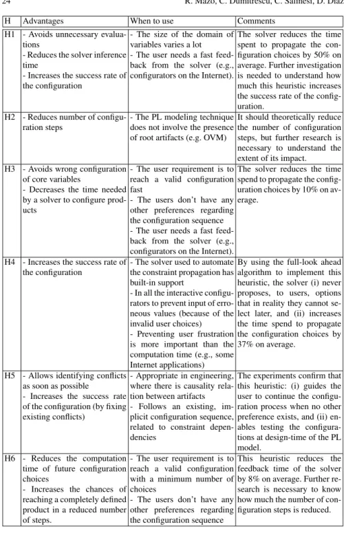
H Advantages When to use Comments H1 - Avoids unnecessary
evalua-tions
- Reduces the solver inference time
- Increases the success rate of the configuration
- The size of the domain of variables varies a lot - The user needs a fast feed-back from the solver (e.g., configurators on the Internet).
The solver reduces the time spent to propagate the con-figuration choices by 50% on average. Further investigation is needed to understand how much this heuristic increases the success rate of the config-uration.
H2 - Reduces number of configu-ration steps
- The PL modeling technique does not involve the presence of root artifacts (e.g. OVM)
It should theoretically reduce the number of configuration steps, but further research is necessary to understand the extent of its impact. H3 - Avoids wrong configuration
of core variables
- Decreases the time needed by a solver to configure prod-ucts
- The user requirement is to reach a valid configuration fast
- The users don’t have any other preferences regarding the configuration sequence - The user needs a fast feed-back from the solver (e.g., configurators on the Internet).
The solver reduces the time spend to propagate the config-uration choices by 10% on av-erage.
H4 - Increases the success rate of the configuration
- The solver used to automate the constraint propagation has built-in support
- In all the interactive configu-rators to prevent input of erro-neous values (because of the invalid user choices) - Preventing user frustration is more important than the computation time (e.g., some Internet applications)
By using the full-look ahead algorithm to implement this heuristic, the solver (i) never proposes, to users, options that in reality they cannot se-lect later, and (ii) increases the time spend to propagate the configuration choices by 37% on average.
H5 - Allows identifying conflicts as soon as possible
- Increases the success rate of the configuration (by fixing existing conflicts)
- Appropriate in engineering, where there is causality rela-tion between artifacts - Follows an existing, im-plicit configuration sequence, related to constraint depen-dencies
The experiments confirm that this heuristic: (i) guides the user to continue the configu-ration process when no other preference exists, and (ii) en-ables testing the configura-tions at design-time of the PL model.
H6 - Reduces the computation time of future configuration choices
- Increases the chances of reaching a completely defined product in a reduced number of steps.
- The user requirement is to reach a valid configuration with a minimum number of choices
- The users don’t have any other preferences regarding the configuration sequence
This heuristic reduces the feedback time of the solver by 8% on average. Further re-search is necessary to know how much the number of con-figuration steps is reduced.
1.6 Conclusion
The purpose of the heuristics was to improve the configuration process by : (i) reduc-ing the number of configuration steps or (ii) reducreduc-ing the computation time required by the solver to test the validity of the product line. The configuration of variables is done interactively by the user. Thus the order depends on their preference. By pri-oritizing choices, and recommending certain configuration variables before others, it is possible to improve these two aspects of the configuration process.
However, other questions may be raised: Which heuristics are better to improve the quality and pertinence of the solutions? Against what other criteria can we use to compare the collection of heuristics presented in this chapter? How to classify the heuristics according to their pertinence in certain situations? What kind of system-atic recommendation should be presented to a user during a product line configura-tion process? How to apply and even combine the collecconfigura-tion of heuristics presented in this chapter, in an interactive and incremental configuration process? In conclu-sion, the application of these heuristics on other product line models, specified with different formalisms can be implemented using the same principles, but may need further evaluation.
References
1. Abbasi, E., Hubaux, A., Heymans, P.: A toolset for feature-based configuration workflows. In: Software Product Line Conference (SPLC), 2011 15th International, pp. 65–69 (2011). DOI 10.1109/SPLC.2011.41
2. Antkiewicz, M., Czarnecki, K.: FeaturePlugin: feature modeling plug-in for eclipse. In: Pro-ceedings of the 2004 OOPSLA workshop on eclipse technology eXchange, eclipse ’04, pp. 67–72. ACM, New York, NY, USA (2004). DOI 10.1145/1066129.1066143
3. Astesana, J.M., Cosserat, L., Fargier, H.: Constraint-based vehicle configuration: A case study. In: 2010 22nd IEEE International Conference on Tools with Artificial Intelligence (ICTAI), vol. 1, pp. 68 –75 (2010). DOI 10.1109/ICTAI.2010.19
4. Batory, D., Benavides, D., Ruiz-Cortes, A.: Automated analysis of feature models: challenges ahead. Communications of the ACM 49(12), 45–47 (2006)
5. Benavides, D., Trinidad, P., Ruiz-Cort´es, A.: Automated reasoning on feature models. In: Advanced Information Systems Engineering, no. 3520 in Lecture Notes in Computer Science, pp. 491 –503. Springer Berlin Heidelberg (2005)
6. Boussemart, F., Hemery, F., Lecoutre, C., Sais, L.: Boosting systematic search by weighting constraints. In: ECAI, vol. 16, p. 146 (2004)
7. Burke, R.: Knowledge-based recommender systems. In: ENCYCLOPEDIA OF LIBRARY AND INFORMATION SYSTEMS, p. 2000. Marcel Dekker (2000)
8. Clements, P., Northrop, L.M.: Software Product Lines: Practices and Patterns. Prentice Hall (2002)
9. Clements, P., Northrop, L.M.: A framework for software product line practice, version 5.0. http://www.sei.cmu.edu/productlines/frame report/introduction.htm (2007). URLhttp:// www.sei.cmu.edu/productlines/frame_report/introduction.htm 10. Deursen, A.v., Klint, P.: Domain-specific language design requires feature descriptions.
11. Dhungana, D., Gr¨unbacher, P., Rabiser, R.: The DOPLER meta-tool for decision-oriented variability modeling: a multiple case study. Automated Software Engineering 18(1), 77–114 (2010)
12. Diaz, D., Codognet, P.: Design and implementation of the gnu prolog system. Journal of Functional and Logic Programming 6(2001), 542 (2001)
13. Djebbi, O., Salinesi, C.: RED-PL, a method for deriving product requirements from a product line requirements model. In: Proceedings of the 19th international conference on Advanced information systems engineering, p. 279293 (2007)
14. Dumitrescu, C., Mazo, R., Salinesi, C., Dauron, A.: Bridging the gap between product lines and systems engineering: an experience in variability management for automotive model based systems engineering. In: Proceedings of the 17th International Software Product Line Conference, SPLC ’13, pp. 254–263. ACM, New York, NY, USA (2013). DOI 10.1145/ 2491627.2491655. URLhttp://doi.acm.org/10.1145/2491627.2491655 15. Dumitrescu, C., Tessier, P., Salinesi, C., Grard, S., Dauron, A.: Flexible product line derivation
applied to a model based systems engineering process. In: Aiguier, M., Caseau, Y., Krob, D., Rauzy, A. (eds.) Complex Systems Design & Management, pp. 227–239. Springer Berlin Heidelberg (2013). DOI 10.1007/978-3-642-34404-6 15. URLhttp://dx.doi.org/ 10.1007/978-3-642-34404-6_15
16. Hadzic, T., Andersen, H.R.: An introduction to solving interactive configuration problems. Tech. rep., Technical Report TR-2004-49, The IT University of Copenhagen (2004) 17. Hadzic, T., Subbarayan, S., Jensen, R.M., Andersen, H.R., Mller, J., Hulgaard, H.: Fast
backtrack-free product configuration using a precompiled solution space representation. small 10(1), 3 (2004)
18. Jiang, Z., Wang, W., Benbasat, I.: Multimedia-based interactive advising technology for online consumer decision support. Commun. ACM 48(9), 92–98 (2005). DOI 10.1145/1081992. 1081995. URLhttp://doi.acm.org/10.1145/1081992.1081995
19. Kang, K.C., Cohen, S.G., Hess, J.A., Novak, W.E., Peterson, A.S.: Feature-oriented domain analysis (FODA) feasibility study. Tech. rep., DTIC Document (1990)
20. Mazo, R., Lopez-Herrejon, R.E., Salinesi, C., Diaz, D., Egyed, A.: Conformance checking with constraint logic programming: The case of feature models. In: Computer Software and Applications Conference (COMPSAC), 2011 IEEE 35th Annual, pp. 456–465 (2011) 21. Mazo, R., Salinesi, C., Diaz, D.: VariaMos: a tool for product line driven systems engineering
with a constraint based approach. In: 24th International Conference on Advanced Information Systems Engineering (CAiSE Forum’12). Gdansk, Pologne (2012)
22. Mazo, R., Salinesi, C., Diaz, D., Djebbi, O., Lora-Michiels, A.: Constraints: The heart of domain and application engineering in the product lines engineering strategy. International Journal of Information System Modeling and Design (IJISMD) 3, 33–68 (2012)
23. Mazo, R., Salinesi, C., Diaz, D., Lora-Michiels, A.: Transforming attribute and clone-enabled feature models into constraint programs over finite domains. In: 6th International Conference on Evaluation of Novel Approaches to Software Engineering (ENASE) (2011)
24. Mendonca, M., Wasowski, A., Czarnecki, K.: Sat-based analysis of feature models is easy. In: Proceedings of the 13th International Software Product Line Conference, SPLC ’09, pp. 231– 240. Carnegie Mellon University, Pittsburgh, PA, USA (2009). URLhttp://dl.acm. org/citation.cfm?id=1753235.1753267
25. Payne, J.W., Bettman, J.R., Johnson, E.J.: The Adaptive Decision Maker. Cambridge Univer-sity Press (1993)
26. Pohl, K., B¨ockle, G., Linden, F.J.v.d.: Software Product Line Engineering: Foundations, Prin-ciples and Techniques. Springer-Verlag New York, Inc., Secaucus, NJ, USA (2005) 27. Robillard, M., Maalej, W., Walker, R.J., Zimmermann, T.: Introduction. In: Robillard, M.,
Maalej, W., Walker, R.J., Zimmermann, T. (eds.) Recommendation Systems in Software En-gineering, chap. 1. Springer (2014)
28. Salinesi, C., Mazo, R., Diaz, D., Djebbi, O.: Using integer constraint solving in reuse based requirements engineering. In: Requirements Engineering Conference (RE), 2010 18th IEEE International, pp. 243 –251 (2010). DOI 10.1109/RE.2010.36
29. Schneeweiss, D., Hofstedt, P.: FdConfig: a constraint-based interactive product configurator. arXiv:1108.5586 (2011). URLhttp://arxiv.org/abs/1108.5586
30. Subbarayan, S.: Integrating CSP decomposition techniques and BDDs for compiling configu-ration problems. In: In Proceedings of the CP-AI-OR. Springer LNCS (2005)
31. Subbarayan, S., Jensen, R.M., Hadzic, T., Andersen, H.R., Hulgaard, H., Mller, J.: Comparing two implementations of a complete and backtrack-free interactive configurator. In: Proceed-ings of the CP-04 Workshop on CSP Techniques with Immediate Application, pp. 97–111 (2004)
32. Thompson, C.A., G¨oker, M.H., Langley, P.: A personalized system for conversational rec-ommendations. JOURNAL OF ARTIFICIAL INTELLIGENCE RESEARCH 21, 393–428 (2002)
33. Van Hentenryck, P.: Constraint satisfaction in logic programming. MIT Press, Cambridge, MA, USA (1989)
34. Winterfeldt, D.V., Edwards, W.: Decision Analysis And Behavioral Research. University Press (1986)