HAL Id: halshs-00196183
https://halshs.archives-ouvertes.fr/halshs-00196183
Submitted on 12 Dec 2007
HAL is a multi-disciplinary open access
archive for the deposit and dissemination of sci-entific research documents, whether they are pub-lished or not. The documents may come from teaching and research institutions in France or abroad, or from public or private research centers.
L’archive ouverte pluridisciplinaire HAL, est destinée au dépôt et à la diffusion de documents scientifiques de niveau recherche, publiés ou non, émanant des établissements d’enseignement et de recherche français ou étrangers, des laboratoires publics ou privés.
Constrained efficiency in the neoclassical growth model
with uninsurable idiosyncratic shocks
Julio Davila, Jay H. Hong, Per Krusell, José-Victor Rios Rull
To cite this version:
Julio Davila, Jay H. Hong, Per Krusell, José-Victor Rios Rull. Constrained efficiency in the neoclassical growth model with uninsurable idiosyncratic shocks. 2005. �halshs-00196183�
Maison des Sciences Économiques, 106-112 boulevard de L'Hôpital, 75647 Paris Cedex 13
http://mse.univ-paris1.fr/Publicat.htm
UMR CNRS 8095
Constrained efficiency in the neoclassical growth model with uninsurable idiosyncratic shocks
Julio DAVILA, CERMSEM– Univ. Pennsylvania & ECARES Jay H. HONG, Univ.Pennsylvania
Per KRUSELL, Princeton University – IIES & CAERP José-Victor RIOS-RULL, PrincetonUniversity & CAERP
Constrained efficiency in the neoclassical growth model
with uninsurable idiosyncratic shocks
Julio Davila
Jay H. Hong
Per Krusell
Jos´e-V´ıctor R´ıos-Rull
∗July 23, 2005
Abstract
We investigate the welfare properties of the one-sector neoclassic growth model with uninsurable idiosyncratic shocks. We focus on the constrained efficiency notion of the general equilibrium literature, and we demonstrate constrained inefficiency for our model. We provide a characterization of constrained efficiency that uses the first-order condition of a constrained planner’s problem that points to the margins of relevance for whether capital is too high or too low: the income composition of the (consumption-)poor. We calibrate our benchmark model parameters governing idiosyncratic risks to the U.S. earnings and wealth distribution, and for this distribution the income of the poor is mainly composed of labor earnings. We compute the constrained-efficient allocations—including transition dynamics—for our model economy, and we conclude that the long-run capital stock in a laissez-faire world is not only too low, but much too low. We also show that one can find parameterizations with different qualitative features: in one case, the steady-state capital stock is too high, and in another case no steady state exists.
∗Davila: CERMSEM, University of Pennsylvania, and ECARES; Hong: University of Pennsylvania;
Krusell: Princeton University, IIES, CAERP; R´ıos-Rull: University of Pennsylvania, and CAERP. We thank Tim Kehoe, John Magill, Iv´an Werning, and Martine Quinzii for very helpful comments. Krusell thanks the National Science Foundation and R´ıos-Rull thanks the National Science Foundation and the University of Pennsylvania Research Foundation for support.
1
Introduction
In this paper we investigate the welfare properties of the one-sector neoclassical growth model with uninsurable idiosyncratic shocks but precautionary savings. This kind of model was originally developed and analyzed by Bewley (1986), ˙Imrohoro˘glu (1989), Huggett (1993), and Aiyagari (1994), and it has become a standard workhorse for quantitatively based theo-retical analysis of macroeconomics and inequality. The framework is mostly used for positive analysis, but in this paper we analyze its normative properties in some depth. In particular, we use a notion of constrained efficiency that is standard in the incomplete-markets litera-ture going back to Diamond (1967), Hart (1975), Stiglitz (1982), and others and argue that, in general, the laissez-faire equilibrium is constrained inefficient.1 That is, we show that if a
planner could simply make consumers save differently, without in any way completing mar-kets or using transfers between agents, i.e., respecting equilibrium budget constraints and competitive price setting, then the planner should do that. This may not come as a surprise per se: prices are endogenous in our economy, and because asset markets are incomplete, agents’ influence on prices leaves room for improvement, even in the absence of transfers between agents.2 However, what is surprising is the direction of the desired improvement,
and the quantitative magnitude of the inefficiency. In particular, we find for a calibrated version of the model that the equilibrium capital stock is too low , and that it is much too low. This challenges the notion that the precautionary-savings model leads to overaccumu-lation of capital. To us, it is also a powerful example of how the incompleteness of asset markets may lead to drastic constrained inefficiency that is both intuitive and quantitatively plausible.
1A notable more recent contribution on this topic is Geanakoplos, Magill, Quinzii, and Dreze (1990). For
a study of idiosyncratic uninsurable shocks from a incomplete-markets, general-equilibrium perspective, see Carvajal and Polemarchakis (2005).
2Though we will not use the term here, this kind of effect is sometimes referred to as a “pecuniary
We first develop the intuition and prove formal results in the context of a finite-horizon setting. In particular, we first look at a two-period model where the generic inefficiency comes out clearly, though in this case there is indeed always capital overaccumulation. The argument is simple. Suppose that consumers face uninsured wage risk in the second period. Rental income, moreover, is not idiosyncratic, given that all agents are initially alike and save the same amount. A lower capital stock will therefore make total individual income less risky for consumers, because it would lower wages and raise capital returns, thus making the part of income that is stochastic smaller. A command for all agents to lower their savings therefore unambiguously improves welfare, and the result is a general one that does not depend on specifics of the utility function or of technology.
In a three-period model, it is already clear, however, that there may be capital under-accumulation in period 2. This is because at that point, those who had lucky labor outcomes will (given that period-t consumption is a normal good) save more, so if aggregate saving in the second period is induced to fall, the higher return to capital in the third period will help those who were lucky in period two and hence be worse from an ex-ante risk perspective. Whether this channel is more relevant for welfare than the effect via wages, which works in the opposite direction, is a quantitative matter, and we use an infinite-horizon model with a parameterization that matches key inequality statistics to examine this issue carefully. The three-period model also makes clear that the constrained optimum may call for different distortions to the savings of different consumers; we later show that these effects can be important both quantitative and qualitatively in the infinite-horizon version of the model.
Our study of the infinite-horizon setting is mainly focused on steady states: we assume that the constrained optimum involves convergence to a steady state, and we then numer-ically examine what such a steady state looks like.3 This analysis is based on a functional
first-order condition that is a necessary condition of the constrained-efficiency planning prob-lem. This first-order condition is, to our knowledge, new, and it is one of the key analytical tools put forth in this paper. Our central finding is that whether there is over- or under-accumulation of capital depends crucially on the factor composition of the income of the
poor agents. If the poor (consumption-poor) agents have labor-intensive income, then the
constrained-efficient allocation involves a larger stock of capital than the market economy delivers by itself. If instead the consumption-poor agents have capital-intensive income, the reverse result holds true. The calibration we employ in the benchmark economy, however, insists on matching central features of the inequality observed in U.S. data—since these are the key features to calibrate to in this kind of analysis—and it delivers a clear message: the consumption-poor are mainly wealth-poor, and hence the planner should increase the capital stock, so that steady-state wages rise. Our calibration is based on Casta˜neda, D´ıaz-Gim´enez, and R´ıos-Rull (2003).
We illustrate that other results may obtain if different parameterizations are entertained. One of these involves a case where the consumption-poor agents have capital-intensive income—here risk can be interpreted as unemployment (and not wage) risk—and here we show that the capital stock should be reduced somewhat from a constrained-efficiency per-spective. We then look at the parameterization originally used by Aiyagari (1994), which delivers too little wage and wealth inequality, and we find that a constrained-efficient steady state does not exist. Here, we use numerical techniques to argue that the constrained opti-mum involves convergence in the total capital stock (to a higher value) and ever-increasing wealth inequality: there is increasing returns to saving from a constrained-efficiency perspec-tive.
An aspect of our results worth emphasizing is that the associated full-insurance, or “first-best”, allocation involves less long-run capital accumulation than does the laissez-faire
out-come. This means that the in-between concept of constrained optimality—which delivers an in-between ex-ante utility outcome and hence more effective insurance than does the laissez-faire economy—demands long-run capital accumulation that is far from in-between. Instead, the constrained optimum finds capital accumulation a convenient vehicle (in the absence of direct insurance transfers) for achieving better insurance indirectly. In this con-text, our quantitative finding also contrasts the statements of Aiyagari (1995) and Aiyagari and McGrattan (1995) that various forms of fiscal policy (taxes on capital/government debt) should be used because there is too much capital in a laissez-faire equilibrium. The argu-ments there are of the standard precautionary-savings nature, and they rely on assuming a form of redistribution (via public goods) or restrictions to proportional taxation. Also, in the present paper the planner has access to state-contingent taxes; we leave restrictions to taxes that are not state-contingent to future work.
Section 2 describes the finite-horizon model and analyzes constrained efficiency in this economy. Section 3 describes the model with an infinite horizon and describes laissez-faire equilibria. The associated constrained-efficiency planning problem is then described in Sec-tion 4 and the central first-order condiSec-tion is derived. SecSec-tion 4.3 briefly discusses a market implementation of the optimal policy, while Section 5 carries out the quantitative analysis for our calibrated infinite-horizon model; the alternative parameterizations are considered in Section 6. Section 7 concludes.
2
The mechanisms: illustration using a finite-horizon model
Though our main aim is a quantitative evaluation of efficiency properties of the typical long-or infinite-hlong-orizon incomplete-markets economy used in the recent macroeconomic literature, the nature of the mechanisms we wish to point to can be discussed within the context of finite-horizon economies. In the present section we therefore first consider a 2-period model,
where we will demonstrate a constrained-inefficiency result—involving over -accumulation of capital—that holds quite generally and that has a natural interpretation. There is another mechanism in the infinite-horizon setting that leads to under -accumulation of capital, how-ever, and it cannot be studied with a two-period setting alone. Therefore, we end the present section with a short discussion of how this mechanism would enter in an economy that lasts for 3 or more periods.
2.1 A 2-period model
Consider an economy with a continuum (measure 1) of ex-ante identical consumers, each living for two periods. The consumers have time-additive, von Neumann-Morgenstern utility functions with a twice continuously differentiable, strictly increasing and strictly concave period utility function u and discount factor β. In the first period, period 1, each agent is endowed with y units of output which can be either consumed, c, or invested, k. In period two, consumers receive income from the capital they saved in period 1 and from working. The labor income of any given individual is random. In particular, the labor endowment can be either high or low, and it is independent across agents. We denote the period-2 labor endowments e1 and e2, with 0 < e1 < e2; the probability that any agent’s labor endowment
is e1 is π. Due to the independence of shocks across consumers, a law of large numbers
operates so that also the fraction of agents with e1 is π. That is, there is no uncertainty
about the period-2 labor endowment: the supply of labor is constant at L = πe1+ (1 − π)e2.
In the second period, output comes from production using capital and labor and a constant-returns-to-scale neoclassical production function f . Since all agents face the same maximization problem, and since this is a problem with a strictly concave objective and a linear constraint set, they will all make identical choices. Let the implied equilibrium choice of capital be K (per consumer, and in the aggregate). Then the output in period 2 is known
to be f (K, L). Output is produced by perfectly competitive firms in our equilibrium: they sell the output to consumers and rent the capital and the labor services from the same con-sumers at rates r and w, respectively. In equilibrium, thus, r and w will be set to equal the marginal products of the inputs; in particular, they will be deterministic. This means that in period 1, each consumer will see his capital income in period 2 as deterministic and equal to rK, whereas his labor income is random and equal to we.
It is a maintained assumption in our analysis that consumers can only save using capital; in particular, there is no pure insurance instrument available for reducing the idiosyncratic risk, so the only way of influencing the risk is through “precautionary savings”.
Given the above, we have
Definition 1. A competitive equilibrium is a vector (K, r, w) such that (i) K solves
max
k∈[0,y]u(y − k) + β (πu(rk + we1) + (1 − π)u(rk + we2))
and (ii) r = fk(K, L) and w = fl(K, L), with L = πe1+ (1 − π)e2.
It is straightforward to show that an equilibrium with K ∈ (0, y) exists under suitable (e.g., INADA) conditions on u and f .
Can the market allocation be improved upon? The notion of constrained efficiency In this economy, agents really only make one choice. Following the incomplete-markets general-equilibrium literature, we discuss the efficiency properties of the equilibrium in terms of whether this one choice could be made in a better way: can it be made so as to improve on equilibrium utility? Formally, we call the equilibrium constrained efficient if there is no level of saving ˆK such that, given competitive pricing of inputs in period 2, the utility of
(K, r, w) we consider is efficient if there is no ˆK ∈ [0, y] such that
u(y − ˆK) + β
³
πu(fk( ˆK, L) ˆK + fl( ˆK, L)e1) + (1 − π)u(fk( ˆK, L) ˆK + fl( ˆK, L)e2)
´
>
u(y − K) + β (πu(fk(K, L)K + fl(K, L)e1) + (1 − π)u(fk(K, L)K + fl(K, L)e2)) .
The question, thus, is whether a fictitious planner can improve on the allocation by simply commanding a different savings level for the representative consumer, while respecting all budget constraints of agents and letting firms operate freely under perfect competition? In particular, the fictitious planner is not allowed to “complete markets” or in any way transfer goods between lucky and unlucky consumers: the only insurance asset is still capital. The market outcome is constrained inefficient: the formal argument In this economy, whether it is possible to improve on the market allocation can be seen by considering the impact of a small variation dK of the aggregate capital. Differentiating the indirect utility one obtains
dU = −uc(y − K)dK + β (πuc(rK + we1)dC1+ (1 − π)uc(rK + we2)dC2) ,
where
dC1 = rdK + Kdr + e1dw
dC2 = rdK + Kdr + e2dw.
The individual’s first-order condition for savings reads
This condition can be used to simplify the above expression, and it will lead many of the effects of increasing capital to vanish. We thus obtain
dU = β µ (πuc(rK + we1) + (1 − π)uc(rK + we2)) Kdr +(πuc(rK + we1)e1+ (1 − π)uc(rK + we2)e2) dw ¶ ,
so that we see that any effect of a marginal change of savings away from the competitive equilibrium has to operate through its effect on factor prices. The cancellations, of course, are just a result of the envelope theorem.
As for how factor prices are affected by capital, we note that
dr = fKK(K, L)dK dw = fKL(K, L)dK so that dU = β µ πuc(rK + we1)(KfKK(K, L) + e1fKL(K, L)) +(1 − π)uc(rK + we2)(KfKK(K, L) + e2fKL(K, L)) ¶ dK.
Now note that because f is homogeneous of degree 1, KfKK(K, L) + LfKL(K, L) = 0 and therefore dU = β µ πuc(rK + we1) ³ 1 − e1 L ´ + (1 − π)uc(rK + we2) ³ 1 − e2 L ´¶ fKKKdK.
parenthesis above becomes πuc(rK + we1) ³ 1 −e1 L ´ + (1 − π)uc(rK + we2) ³ 1 −e2 L ´ =
πuc(rK + we1) + (1 − π)uc(rK + we2) − (ˆπuc(rK + we1) + (1 − ˆπ)uc(rK + we2))
= (π − ˆπ)(uc(rK + we1) − uc(rK + we2)) > 0
because e2 > e1 and π − ˆπ = π(1 − (e1/L)) > 0. Therefore, for dK > 0, since fKK < 0,
dU = β(π − ˆπ)(uc(rK + we1) − uc(rK + we2))fKKKdK < 0.
We conclude, in other words, that the equilibrium is constrained inefficient. As is clear from the analysis, the key assumptions behind the result is that u is strictly concave and that f has a strictly decreasing marginal product of capital.
More specifically, the level of capital in the laissez-faire equilibrium is too high: a higher utility is obtained if all consumers save a little less in period 1. The intuitive reason for the overaccumulation of capital is as follows. More capital savings raises wages and lowers rental rates. The only source of market failure in this economy is the incomplete insurance. A small decrease in K from the equilibrium level thus lowers w and raises r, thereby scaling down the part of the consumer’s income that is stochastic and scaling up the part that is deterministic: the amount of risk the consumer is exposed to is now smaller. Given that there is no direct insurance for this risk, this amounts to an improvement. The “distortion” on the agents’ savings by moving savings away from the competitive-equilibrium level for given prices is of a second-order magnitude, and thus the manipulation of prices so as to lower the de-facto risk dominates.
the complete-markets case, prices are not optimally set here and agents’ influence on prices should therefore be taken into account when making individual choices. An improvement on the competitive outcome thus requires taking an aggregate, “planning” perspective.
2.2 More periods
In the two-period model, apparently, our overaccumulation result obtains rather generally. Our main focus here, however, is longer-lived economies; indeed, the next section of the paper examines the typical macroeconomic setting with an infinite time horizon. But before we discuss the infinite-horizon model in detail, what additional mechanisms appear in longer-horizon models? In this section we will use a three-period model, where there are neoclassical production and idiosyncratic labor endowment shocks both in periods 2 and 3, to illustrate how the analysis of constrained efficiency changes with more periods.
Over- or under-accumulation? Following the analysis of the 2-period model, one can study the optimal savings decision in the intermediate period 2. Now there are two kinds of agents to consider: those who had a high labor endowment realization in this period, and those who had a low one. Specifically, one can look at whether an increase in the aggregate capital stock carried from period 2 into period 3 will raise the utility of consumer i, where i refers to the labor endowment realization in period 2. As before, utility is only influenced through the price effects, and the impact on consumer i’s equilibrium present-value utility can be derived in a straightforward manner along the lines of the above analysis. This impact is
dUi = β2 µ πuc(rKi+ we1) µ Ki K − e1 L ¶ + (1 − π)uc(rKi+ we2) µ Ki K − e2 L ¶¶ fKK(K)KdK.
where for simplicity the notation has been maintained—K, L, r etc. refer to third-period values—and the idiosyncratic shocks have been assumed to be iid. Moreover, Ki refers
to the savings of the consumer with an i shock, where now K1 < K2 is expected, since
type-2 consumers are richer ex post. Inspecting this expression, we see that a decrease in capital—which is unambiguously beneficial in a 2-period economy—is a plus for type-2 agents and a minus for type-1 agents, since K2 > K > K1. Moreover, note that the
planner maximizes period-0 utility, which makes the de-facto weight on type-1 agents larger, because their marginal utilities in the third period are lower due to their lower savings:
uc(rK1 + wej) > uc(rK2 + wej) for j = 1, 2. This means that we have uncovered a reason why a decrease in savings may be detrimental: the implied increase in the rental rate in
period 3 will help those who are lucky in period 2 , thus making the lack-of-insurance problem
more severe. This effect, as it turns out, will under some calibrations be more important quantitatively than the direct effect that is present in the 2-period model. In the next section, we will discuss what features of the economy are key for whether aggregate equilibrium savings are too high or too low. in that section we will, moreover, derive a first-condition for savings that comes from maximizing consumer welfare subject to the given market structure and that allows us to talk also about the “best” level of savings. That first-order condition in particular summarizes the conflicting effects on savings.
Who should save? Another interesting aspect of our efficiency analysis—that will also play a central role in one of our examples in the next section—is that there are nontrivial distributional implications for what a planner should do. In particular, the constraints on what the planner can do to improve utility do not rule out choosing the savings of the two consumers with different labor endowment realizations in period 2 separately. In the above discussion, we increased aggregate capital and it was implicit that all agents’ savings were increased by equal amounts. Would the planner command lucky consumers to save more or less than unlucky consumers? The general idea here is that (i) agents that are “lucky” are agents with ex-post low marginal utility and therefore (ii) agents with low marginal utility
have lower marginal costs of increased savings (and lower marginal benefits of decreased savings). As an example, if the pecuniary externality of savings that exists in this model is positive—so that more aggregate saving is desirable—the planner would want to make ex-post lucky agents increase their savings more than unlucky agents. Hence, we would obtain an argument for increased differences in asset inequality. Of course, this increase in asset inequality is no redistribution from unlucky to lucky consumers, and indeed consumption early on becomes less dispersed, because the whole point is that ex-post utilities should become less dispersed.
3
The infinite-horizon economy
We now study the infinite-horizon model. In essence, it is a long-horizon version of the economy described above.
3.1 The economy and recursive competitive equilibrium
As above, we look at a continuum of agents subject to idiosyncratic shocks ei ∈ E, where
E ≡ {e1, · · · , ei, · · · , eI}, that are i.i.d. across agents and that follow a Markov process
with transition matrix πi,j. These shocks are the amount of efficient units of labor that agents have each period. Agents have standard preferences: an expected discounted sum of a strictly increasing and strictly concave utility function, i.e., E0 {
P
t βt u(ct)}. Agents do not have access to state-contingent contracts but can only accumulate assets in the form of real capital; we denote it a. There is a lower bound on assets: a.4 We assume a borrowing
constraint that prevents these assets from being negative. Moreover, we assume a very large upper bound on assets, a, implying a ∈ A = [0, a]. As in the previous section, these assets
4This lower bound may arise from the existence of a solvency constraint that requires that agents are
always able to pay back their debt or from an explicit borrowing constraint. The latter is used in the popular case that restricts assets to be nonnegative.
are rented by competitive firms each period and used for production purposes according to a constant-returns-to-scale neoclassical production function f that uses capital and efficient units of labor. Capital accumulation is assumed to follow a geometric structure: a fraction
δ of the capital stock depreciates from one period to the next.5
The nature of the budget constraint that agents face is thus
c + a0 = a (1 + r) + e w (1)
where we use primes to denote next period’s values and where r and w are the rental prices of capital and labor that have yet to be determined.
Individual agents are indexed by the pair {e, a} that describes their labor endowment and wealth, respectively. The state of the economy can be summarized by means of a probability measure x over the Borel sets of compact set S = E × A. In this context, aggregate amounts of factors of production and their rental prices are
K = Z S a dx, r = fK(K, L) − δ, (2) L = Z S e dx, w = fL(K, L), (3)
and we write r(x) and w(x). On occasion we also write r(K) and w(K) since aggregate labor L is constant due to the law of large numbers.
In this economy the aggregate state variable is the distribution of agents over labor earnings and wealth, x, which agents have to know in order to compute prices.6 We write
5Note that the assumptions in the previous section can be thought of as assuming 100% depreciation, or
that alternatively f was defined to include undepreciated capital.
6While prices today can be known just from today’s aggregate capital, future prices cannot be known from
today’s aggregate capital because decision rules are not linear. Hence the distribution is the appropriate state variable. See Krusell and Smith (1997), Krusell and Smith (1998), or R´ıos-Rull (1998) for more elaborate discussion.
x0 = H(x) to describe the law of motion of the distribution. Then, the agent’s problem is v(x, e, a) = max c≥0 a0∈A u (c) + β X e0 πe,e0 v(x0, e0, a0) s.t. (4) c + a0 = a [1 + r (x)] + e w (x) , (5) x0 = H(x), (6)
with solution a0 = h(x, e, a). An important feature of this problem is the requirement that the agent’s assets lie in compact set A.
We now turn to the construction of an aggregate law of motion of the economy. Using decision rule h and transition matrix π, we construct an individual transition process. Let
B ∈ S be a Borel set. Define Q by
Q(x, e, a, B; h) = X
e0∈Be
πee0 χh(x,e,a)∈Ba (7)
where χ is the indicator function. It is easy to see that Q is indeed a transition function. We now define the updating operator T (x, Q) that yields tomorrow’s distribution given today’s:
x0(B) = T (x, Q)(B) = Z
S
Q(x, e, a, B; h) dx (8)
An equilibrium requires that agents expectations are correct. Formally,
Definition 2. A recursive competitive equilibrium is a pair of functions h and H such that
h solves problem (4) given H and that H(x) = T (x, Q(.; h)).
A steady state for this economy is a distribution ex such that ex = T (ex, Q). Steady states
the aggregate capital stock is higher than that of an economy with perfect markets or no shocks (for a discussion and a proof of this result, see Huggett (1997)). The interpretation of this result is one of precautionary savings: savings play dual roles here, by not just allowing intertemporal smoothing but also some (limited) amount of smoothing across states.
3.2 Characterization: first-order conditions and steady-state capital
In a recursive competitive equilibrium, the consumer’s first-order condition for savings is
uc(a [1 + r (x)] + e w (x) − a0) ≥ β X
e0
πe,e0 v3(x0, e0, a0) (9)
with equality if a0 > a. The envelope condition is
v3(x, e, a) = [1 + r(x)] uc(a [1 + r (x)] + e w (x) − a0) . (10)
Combining the two conditions and using the economy’s law of motion and the agent’s decision rule, we obtain
uc(x, e, a, h(x, e, a)) ≥ β [1 + r(H(x))] X
e0
πe,e0 uc(H(x), e0, h(x, e, a), h[H(x), e0, h(x, e, a)]) , (11)
which can be rewritten compactly as
uc ≥ β [1 + r(H(x))]
X e0
πe,e0 u0c. (12)
Steady states can be readily found by finding a fixed point of an aggregate steady-state capital demand function, which depends on the interest rate which in turn is given by the
marginal productivity of capital (see below). Let hm(e, a; r) be the decision the rule implied by a constant interest rate r (and associated wage w). It solves
uc[a (1 + r) + e w − hm(e, a; r)] ≥
β X
e0
πe,e0 uc[hm(e, a; r) (1 + r) + e w − hm[e0, hm(e, a; r); r]] , (13)
with equality if hm > a.
Let the stationary aggregate capital implied by hm(., .; r) be K(r), a continuous function of r (R´ıos-Rull (1998)). A steady state is therefore characterized by a ¯K and a rate of return
¯
r such that given ¯r, aggregate capital is ¯K, i.e., ¯K = K(¯r), and ¯r is the marginal productivity
of capital implied by ¯K, i.e. ¯r = fk( ¯K, L). In a steady state, where the discount rate exceeds the interest rate, there is an upper bound to the assets that agents hold (see Huggett (1997)) so the upper bound assumed to exist is not exogenously imposed but generated by the model.
4
Constrained-optimal allocations in the infinite-horizon economy
Though our focus will be on optimal steady states, we have in mind an initial condition like the one in the 2-sector economy: all agents start out alike. I.e., we have in mind a pure insurance problem where the objective of the planner, beside the standard objective of accumulating capital, is to make sure that agents save so as to minimize the losses due to missing insurance markets. Hence a possible interpretation of the planner’s concerns is that it takes the effects of prices explicitly into account. Under complete markets, the effects of consumers’ savings on prices could be ignored, because of the first welfare theorem, but here they cannot.
Our main characterization result—the first-order condition below—is derived using a variational approach and thus based on a sequential formulation of the constrained-efficiency
problem. However, for descriptive purposes, we use a recursive formulation of this planning problem in the main text. It reads
Ω(x) = max y(e,a)∈A
Z S
u [a(1 + r (K)) + e w (K) − y(e, a)] dx + β Ω(x0) (14)
s.t. x0 = T (x, Q(.; y)), K =
Z S
adx. (15)
We use the function h∗ to denote the implied decision rule for y(e, a) at x: a0 = h∗(x, e, a). This recursive program weighs all agents’ utilities equally: it appears “utilitarian”. This specification follows from two assumptions. First, we have in mind an initial condition where all agents are identical: at time 0 they have identical wealth and identical wage status.7 Second, given that consumers are identical at time 0, we assign equal weights to
them, because we wish to study a pure insurance problem and not treat identical consumers differently.8 Because we have this guidance in choosing weights, we are thus able to make
precise statements about the nature of constrained-optimal long-run outcomes.
4.1 The first-order condition
For convenience, we will now assume that the distribution x admits a density.9 Our key
analytical characterization in this paper is the first-order conditions for the planner:
Proposition 1. If the distribution x admits a density, the first-order necessary conditions
7With equal wage status for all agents in the initial period, aggregate labor will not be constant over
time, but it will transit exogenously and deterministically and, due to the law of large numbers, converge to a constant. For simplicity, in the statement of the recursive program above, we presume that aggregate labor is always constant—since we focus our analysis below on long-run outcomes, this simplification is not restrictive.
8It is possible, of course, to imagine different initial conditions. In such cases, however, it would be less
clear how to assign weights to the different agents.
9That our characterization is possible to carry out without this assumption was kindly pointed out to us
of problem (14) can be stated as the following functional equation in the decision rule h∗: for all {e, a} ∈ S, uc(a [1 + r (K)] + ew (K) − h∗(x, e, a)) ≥ β [1 + r (K0)]X e0 πe,e0uc(h∗(x, e, a) [1 + r (K0)] + e0w (K0) − h∗(x0, e0, h∗(x, e, a)]) + β Z S [e0fLK(K0, L)) + a0fKK(K0, L)] uc(a0 [1 + r (K0)] + e0w (K0) − h∗(x0, e0, a0)) dx0 (16)
where the inequality becomes equality if h∗(x, e, a) > a.
Proof. See Appendix A.
For later reference, we will define Y as the implied law of motion of the distribution:
x0 = Y (x) = T (x, Q(.; h∗)).
Omitting arguments, we can write the first-order condition compactly as
uc≥ β (1 + r0) X e0 πe,e0 u0c + β Z S [e0 fLK0 + a0 fKK0 ] u0c dx0. (17)
This equation is the guide for individual savings at different values for (e, a). Thus, it can be compared to equation (12), which characterizes the laissez-faire allocation. We see that the difference between the equations is the third and last term of (17); it was not present in (12) (the other two terms are common). The new term has a number of noteworthy features that change incentives in interesting ways and lie behind the quantitative findings that we present in the quantitative part of the paper.
1. This kind of new term would also appear in finite-horizon models. In the two-period model, the condition is identical in form to the one above, but with (i) h∗ being the same for all agents in the first period since they all start out the same; and (ii) savings being zero for all agents in the second period.
2. The new term captures the additional average effect on utility from increased savings
that is accomplished through price changes. It is thus the sum of tomorrow’s changes
in total income weighted by the marginal utilities of the different agents receiving the income. These weights are higher the lower are the consumption levels of the corresponding consumers.
3. In a representative-agent special case the new term is zero, and hence the equilibrium is constrained-optimal (as it should be, given that the first welfare theorem applies in that case). To see this, note that representative-agent model collapses the integral with respect to wealth yielding
uc≥ β (1 + r0) X e0 πe,e0 u0c + β X e0 πe,e0 [L0 fLK0 + K0 fKK0 ] u0c.
But the terms within brackets sum to zero by the Euler theorem since the production function is homogeneous of degree 0.
4. The new term can be either positive or negative. Its sign is particularly influenced by the sign of the term in brackets for the high marginal utility agents—the consumption-poor agents—since they receive a higher weight. Since the correlation between income and wealth (and thus consumption) is less than one, which of the two variables de-termines the relevant notion of poverty depends on the persistence properties of the shocks. Roughly speaking, the optimal plan assigns consumption poverty to those agents who are the likeliest to be hit by the borrowing constraint in the future.
5. If poor agents have labor-intensive income relative to the economy as a whole then the term in brackets is positive for them, because of the Euler theorem, and then with enough poor agents so is the whole new term. Consequently, the sign of the new term, and thus whether there is too much capital or too little capital in this economy,
depends to a large extent on whether the poor agents’ income is labor-intensive or capital-intensive. If it is labor-intensive, they would benefit from more capital, since
it would raise their total income, and the planner would therefore like to have more capital than the market economy.
6. Whether poor people have labor-intensive income or capital-intensive income is a result of the primitives of the model, but in a quantitatively restricted model these primitives
of course have to be selected to match the relevant economic data. To briefly see this,
imagine that e is i.i.d. and it can take two values, one of these being very unlikely and very small (say, “unemployment”). In such an economy agents save to prevent suffering from low consumption in that state. When the state arrives, thus, labor income is very low while capital income is high in relative terms. As a result, the poor’s income is capital-intensive, and hence the planner would want less capital than what the market allocates. Alternatively, in model economies with a substantial right tail for earnings, wealthy people will mainly be capital rich, and poor people mainly capital poor. Thus, whether the new term is positive or negative is an empirical issue. We discuss this in detail in Section 5, where we both propose a reasonable calibration and illustrate how alternative parameterizations give different results.
7. Finally, the new term is independent of the consumer’s wealth/wage status, and therefore its effect on behavior—its distortionary impact relative to the laissez-faire benchmark—is larger for agents with low marginal utility. In other words, it
wealth distribution. Thus, it suggests that when capital is too low in equilibrium, the increases in savings will be executed mostly by the rich who, as a consequence, suffer lower consumption. This is, of course, part of a desired imperfect measure to improve insurance. We will see below that this mechanism can be very powerful quantitatively and even lead to ever-widening asset inequality. Conversely, when there is too much capital, the decrease in savings will also be disproportionately borne by the rich; here as well, the rich are forced to a larger deviation from what their savings would be absent government intervention.
4.2 The constrained-efficient steady state
We now turn to characterizing the steady state of this economy. A steady state for the planner is a decision rule ¯h∗ and an associated distribution ¯x∗ such that ¯x∗ = Y (¯x∗) and ¯h∗(e, a) = h∗(¯x∗, e, a). With ¯K∗ ≡R
S a d¯x∗, a steady state satisfies
uc ¡ a £1 + r¡K¯∗¢¤+ e w¡K¯∗¢− ¯h∗(e, a)¢ ≥ β [1 + r( ¯K∗)]X e0 πe,e0 uc ¡
¯h∗(e, a)£1 + r¡K¯∗¢¤+ e0 w¡K¯∗¢− ¯h∗(e0, ¯h∗(e, a))¢ + Z S £ e0 f LK( ¯K∗, L) + a0 fKK( ¯K∗, L) ¤ uc ¡ a0 £1 + r¡K¯∗¢¤+ e0 w (K∗) − ¯h∗(e0, a0)¢ d¯x∗. (18) This is a functional equation that can be solved using standard numerical methods. Note in this context that if the last term is positive, there is no guarantee that there exists an upper bound to individual asset holdings. However, an upper bound can be imposed, and in the numerical simulations one would then verify whether or not it is violated.
It is important to note, in this context, that the object of study in our steady-state analysis is a “modified Golden Rule”, i.e., a long-run outcome that is optimal from the perspective of taking discounting into account. In other words, our constrained-optimal steady state is not derived simply from maximizing steady-state utility without regard to initial conditions and the costs or benefits of reaching that steady state. Instead, it answers the question: if the allocation that is ex-ante constrained optimal has the property that there is convergence to a steady state, what are the properties of the implied steady-state distribution?
4.3 Implementation of the constrained optimum
The allocation chosen by the planner involves no transfers between agents and is not im-plementable with mechanisms of an aggregate nature: the planner “instructs” each agent, conditional on asset holding and wage realization, how to save. In order to replicate this command allocation, hence, it is necessary for a government to use taxes and lump-sum transfers that are type-dependent, so that the requirement of no net transfer among agents can be met. Thus, we can think of this as (i) a distortion to saving, using a tax schedule that is nonlinear, i.e., where marginal rates vary with wealth, and that is also type-dependent, i.e., varying with the wage realization, together with (ii) a lump-sum transfer that ensures that the net transfer is zero.
While the mentioned policies can be readily computed from the solution to the planner’s problem, they should not be viewed as a proposal for an actual tax package. The reason is that in general (but not always) they rely on type-specific information, and given this information the government could do even better: it could implement the transfers we do not allow, and thus fully insure agents. A special case in which the constrained-optimal policy would actually correspond to a policy that does not require type-specific information
can be found in the two-period example we discussed first. There, the constrained optimum can be implemented with an investment subsidy in the first period. That is, suppose that the government cannot tax or transfer at all in the second period, but that agents can costlessly trade anonymously in the markets for capital and labor in period two. Then the very best allocation that can be achieved with government intervention is the constrained optimum we compute.
It is an open question how more restrictions (or, more generally, other restrictions) on government policy, such as forcing tax schedules to not depend on the wage realization, would change the characterization. The purpose of this paper is the more narrow one of pinning down the exact nature of how agents, by not taking into account how their decisions influence prices, make decisions that are not optimal from the perspective of risk sharing under the kind of market incompleteness considered in Bewley-type economies. We find the questions about implementable policy interesting, of course, but postpone them for future inquiry.
5
Quantitative analysis: an economy calibrated to match the U.S.
earnings and wealth distribution
Our main focus is on a model economy calibrated so that the steady state of the market allocation generates an earnings and wealth distribution like that in the U.S. as reported in recent SCF surveys. We follow Casta˜neda, D´ıaz-Gim´enez, and R´ıos-Rull (2003) and Diaz, Pijoan-Mas, and R´ıos-Rull (2003) in the detailed modeling. Preferences are of the CRRA form,Ptβt c1−σt −1
1−σ , with the period set to be one year. Production occurs through a standard
neoclassical production function F (Kt, Lt) = Ktθ L1−θt .
earnings distribution is 0.2, with a Gini index of 0.11. The corresponding values of the coef-ficient of variation and the Gini index for the U.S. economy are 2.65 and 0.61, respectively.10.
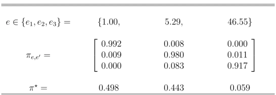
This is one reason why the wealth distribution in the Aiyagari parameterization does not at all look like the actual U.S. wealth distribution. In our calibration here, a key requirement is that not only the dispersion of earnings but also that of wealth are realistic, so we need to move away from Aiyagari’s parameterization. Though there are several possibilities here, we will focus on a simple way of achieving the goal: we follow the calibration described in Diaz, Pijoan-Mas, and R´ıos-Rull (2003), which is a simplified version of that in Casta˜neda, D´ıaz-Gim´enez, and R´ıos-Rull (2003). More precisely, a properly chosen 3-state Markov chain allows us to generate a laissez-faire steady state with inequality measures for earnings and wealth quite close to those in the U.S. data. We report the earnings process that we use in Table 1 below.
Table 1: Earnings process
e ∈ {e1, e2, e3} = {1.00, 5.29, 46.55} πe,e0 = 0.9920.009 0.000 0.008 0.980 0.083 0.000 0.011 0.917 π? = 0.498 0.443 0.059
The table reveals that in order to generate a high Gini coefficient with just three points in the Markov chain, each state must be very different: the labor earnings of the lucky households is almost 50 times those of the unlucky ones. The process for earnings that we use has a Gini index of 0.60.
10The earnings data used by Aiyagari (1994) comes from the PSID which misses the right tail of both the
In addition, the high earnings variability market economy is calibrated so that the steady state of the market economy has an interest rate of 4%. The capital-output ratio is slightly below 3 and the labor share is 0.64, which is accomplished assuming that β = 0.887, δ = 0.8, and θ = 0.36. The intertemporal elasticity of substitution is set to 0.5.
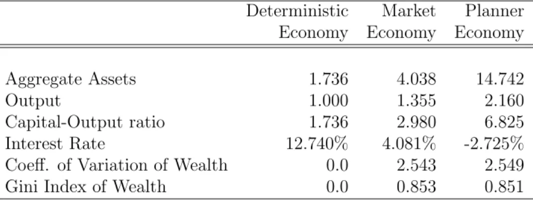
The results for the economy calibrated in the manner just described are contained in Table 2.
Table 2: The steady states for the baseline model economy Deterministic Market Planner
Economy Economy Economy Aggregate Assets 1.736 4.038 14.742
Output 1.000 1.355 2.160
Capital-Output ratio 1.736 2.980 6.825 Interest Rate 12.740% 4.081% -2.725% Coeff. of Variation of Wealth 0.0 2.543 2.549 Gini Index of Wealth 0.0 0.853 0.851
The first column of the table reports the steady states of the deterministic version of the economy (the “first best” when all income shocks are perfectly insured), the second column reports the steady state of the incomplete-markets allocation, and the third column shows the steady state of the constrained-efficient allocation. In this table, TFP was normalized so that output in the deterministic version of the model is 1.
The first notable result is that the market economy has large precautionary savings: aggregate wealth is 2.33 times larger than in the economy without shocks. As a result of the additional capital output is 35.5% higher. We see also the that the Gini index of the market economy is quite large, 0.853, slightly larger than the 0.803 of the U.S. economy.
does the deterministic economy, but the constrained optimum implies an even higher level of capital: it is a whopping 8.5 times higher than in the deterministic economy and even 3.65 times higher than in the market allocation. This is an enormous difference. Moreover, it is a nontrivial finding in that it contradicts the intuition that the “in-between” allocation in an efficiency sense—the allocation improves on laissez faire but is dominated by the first best—should produce an “in-between” amount of long-run capital.
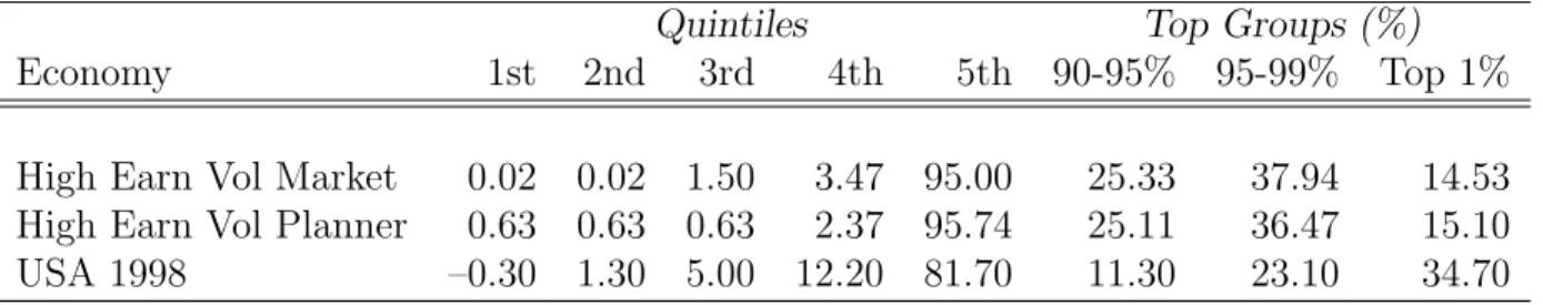
Table 3: The distribution of wealth in the baseline model economy
Quintiles Top Groups (%)
Economy 1st 2nd 3rd 4th 5th 90-95% 95-99% Top 1% High Earn Vol Market 0.02 0.02 1.50 3.47 95.00 25.33 37.94 14.53 High Earn Vol Planner 0.63 0.63 0.63 2.37 95.74 25.11 36.47 15.10 USA 1998 –0.30 1.30 5.00 12.20 81.70 11.30 23.10 34.70
Table 3 shows the share of wealth held by selected groups in both the market and the constrained-optimal allocation of the model economy as well as in U.S. data. We see that the high earnings inequality in the model economy exaggerates the wealth concentration of the U.S. as measured by the share of wealth of the highest quintile, although it generates a lower share of wealth held by the top 1%, which is a little less than one half of that in the data. This is a compromise that comes from the fact that we are using a very parsimonious income process; not all statistics can be targeted. What Table 3 shows is that the wealth distribution of the market and the constrained-optimal allocations are very similar, save for the enormous difference in total assets held.
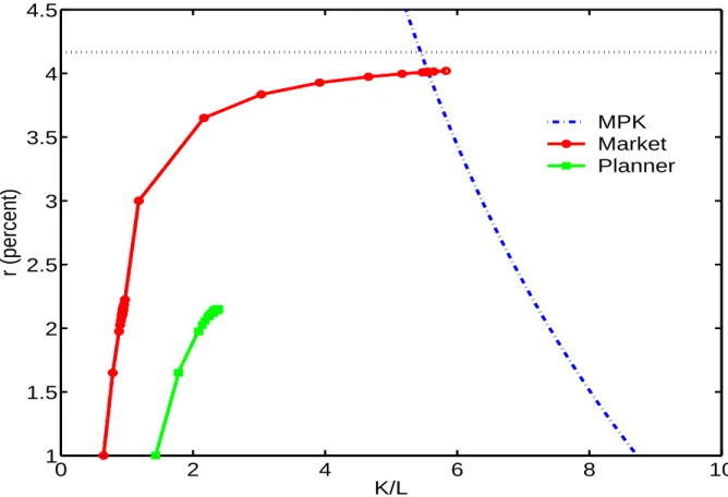
Figure 5 describes key mechanisms in the model; it derives aggregate long-run supply and demand relationships for capital as a function of an interest rate that is assumed constant over time: what total savings would be, and what total demand by firms would be, respectively. The interest rate associated to the economy with full insurance is indicated with
dis-0 5 10 15 20 25 −2 0 2 4 6 8 10 12 14 K/L
r (percent)
MPK Market PlannerFigure 1: Steady-state capital supplies and demands for the market and constrained-efficient economies
continuous lines. The demand for capital is just the schedule for marginal productivity schedule, while the supply of capital is the amount of aggregate asset holdings with respect to the stationary distribution generated by each interest rate. For the constrained-optimal economy, the steady-state supply of capital is based on a calculation where, for each interest rate, the relevant value of the third term of equation (18), denoted g, is solved for given the stationary distribution. This involves a fixed point: given a guess on r and g, one computes a stationary distribution, which delivers updated values for r and g.
To summarize, the constrained-efficient allocation in the model economy has much more capital than does the laissez-faire allocation (which itself has much more capital than does the first-best allocation—due to precautionary savings), despite the fact that the distribution
of wealth as measured by the shares owned by the various groups is very similar. Said differently, the precautionary-savings economy generates too little capital.
6
Other model economies with interesting properties
We now describe two additional model economies. These are less satisfactory in terms of matching the U.S. data, but they illustrate some of the basic mechanisms present in this economy. One of these illustrates that the steady-state level of capital is not always too low, whereas the second illustrates that the constrained optimum may be inconsistent with a stationary wealth distribution.
6.1 The unemployment economy
The first economy is one where the idiosyncratic shock captures unemployment risk rather than wage risk: it can take only two values, with a very low value of unemployment to ensure that the income of the unlucky consumers, i.e., of the unemployed, is capital-intensive. We calibrate the economy to an unemployment rate of 5% and an average duration of unem-ployment of 2.6 years. The parameters involved are e = [0.011.00] for the labor endowment (unemployed, employed) and Π1,· = [0.620.38] and Π2,· = [0.020.98] for the transition matrix.
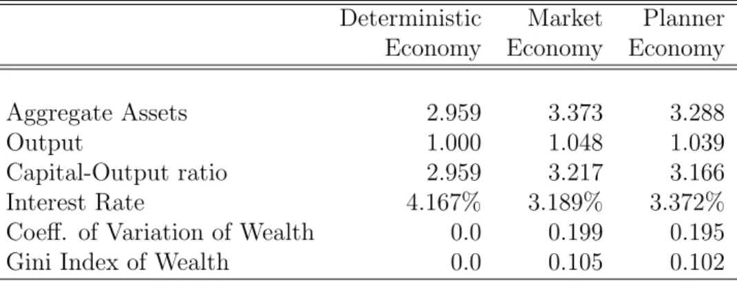
Table 4 displays the steady states of the full-insurance economy, market economy, and the constrained-efficient economy.
The constrained optimum implies a lower long-run level of capital than what is generated by the market alone. This supports the notion that the key determinant is the factor com-position of the income of the poor. In this model economy the poor are unemployed, and their labor income is essentially zero. This makes it de-facto capital-intensive. As part of the calculations, we obtain a value for g (the third term in equation (18)) of -0.001147. The condition g < 0 is indeed the condition that ensures less capital in the constrained optimum
Table 4: The steady states of the unemployment economy Deterministic Market Planner
Economy Economy Economy Aggregate Assets 2.959 3.373 3.288
Output 1.000 1.048 1.039
Capital-Output ratio 2.959 3.217 3.166 Interest Rate 4.167% 3.189% 3.372% Coeff. of Variation of Wealth 0.0 0.199 0.195 Gini Index of Wealth 0.0 0.105 0.102
than in the laissez-faire equilibrium. As a further illustration of the features of this economy, Figure 2 shows the steady-state capital supplies and demands for the laissez-faire as well as constrained-efficient versions of this economy (the full-insurance level of capital is also indicated in the figure: the discontinuous line).
Note that the constrained-efficient supply of steady-state capital is only lower than the market supply of capital for some interest rates—for some interest rates it is higher.
6.2 No constrained-efficient steady state: the original Aiyagari parameterization We now explore an economy that will turn out not to have a constrained-efficient steady state.11 This economy is calibrated to the process for earnings considered in Aiyagari (1994),
whose parameterization mainly originates from PSID data. We follow Aiyagari very closely; in his model economy, there are very few agents in the right tail the earnings distribution, and the wealth distribution is far from that observed in U.S. data.
We specify the parameters so that the economy with complete markets (the standard
11The discussion in this section presumes that no upper bound is imposed on agents’ asset choices. If
such a bound is (arbitrarily) imposed, a steady state does exist in which this upper bound binds for a non-negligible subset of agents.
3 4 5 6 7 8 9 1.5 2 2.5 3 3.5 4 4.5 K/L
r(percent)
MPK Market PlannerFigure 2: Steady-state capital supplies and demands for the market and constrained-efficient unemployment economies
neoclassical growth model) satisfies the standard properties. The interest rate is set to 4.167%: β is 0.96). Our only departure from Aiyagari (1994) is to set the intertemporal elasticity of substitution, 1
σ, to be equal to 0.5.12 The capital share is equal to 0.36 and the capital-output ratio is set to slightly under 3 (actually to 2.959 so that the depreciation rate of capital δ equals 0.08).
With respect to the process for earnings, Aiyagari (1994) assumes an AR(1) in the loga-rithm of labor income. The process is fully described by two properties: its persistence and
12Aiyagari (1994) considers the values 1, 0.33, and 0.2. Ghez and Becker (1975) and MaCurdy (1981),
both using a life cycle model and explicitly accounting for leisure, assume much lower values. Mehra and Prescott (1985) and Prescott (1986) discuss other estimates in the literature and conclude that a reasonable number is not too far from 1. Cooley and Prescott (1995) argue that this parameter is very difficult to pin down but also settle for a value of 1. Hurd (1989) has a point estimate below one.
its volatility. Aiyagari (1994) chooses both values following estimates from Kydland (1984), who used PSID data, and from Abowd and Card (1987) and Abowd and Card (1989), who used both PSID and NLS data. Then, Aiyagari approximates this process using a seven-state Markov chain following the procedures described in Tauchen (1986). We follow the same procedure, although we reduce the Markov chain to three states. We take our benchmark to have an autocorrelation of 0.6 and a coefficient of variation of 0.2.13 In Table 5, we report
the parameter values of the Aiyagari (1994) model economy. The steady state of the market Table 5: Parameter values of the Aiyagari (1994) model economy
General β σ θ δ Parameters 0.96 2 0.36 0.08 e ∈ {e1, e2, e3} = {.78, 1.00, 1.27} Earnings πe,e0 = 0.660.28 0.07 0.27 0.44 0.27 0.07 0.28 0.66 Stat. Distribution π? = 0.337 0.326 0.337
economy has 2.03% more assets and 0.70% more assets that its full-insurance counterpart, with an interest rate of 4.011% instead of the 4.167%. The implied coefficient of variation of wealth is 0.718 and its Gini Index of wealth is 0.388, far below the dispersion observed in data.14
The interesting feature of this economy, however, is that the planner’s problem does not have a steady state. To understand this result, we first displays the aggregate steady-state capital demands and supplies for various interest rates for the market and the constrained-efficient economies: see Figure 3.
0 2 4 6 8 10 1 1.5 2 2.5 3 3.5 4 4.5 K/L
r (percent)
MPK Market PlannerFigure 3: Steady-state capital supplies and demands for the Aiyagari (1994) economy. A steady state requires the intersection of the demand curve with the supply curve of the planner. But the latter is not defined beyond a certain interest rate, which is around 2.15% in the picture. Thus no intersection exists.
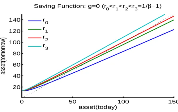
To understand this feature, it is convenient to first look more closely at the individual savings functions of market economies, as indexed by different constant interest rates. These are shown in Figure 4.
Since g = 0 underlies these savings functions—the market does not take into account the additional term that is in the first-order condition of a constrained-efficient allocation. of 0.2 and 0.4.
0 50 100 150 20 40 60 80 100 120 140 asset(today)
asset(tomorrow)
Saving Function: g=0 (r 0<r1<r2<r3=1/β−1) r 0 r 1 r 2 r 3Figure 4: Market savings functions for different values of r.
As the interest rate rises, so does the intersection between the savings function and the diagonal (45-degree line). As the interest rate approaches the inverse of the discount rate the intersection goes to infinity, but for any interest rate below this value there is a finite intersection (see Huggett (1997) for a formal verification of this feature).
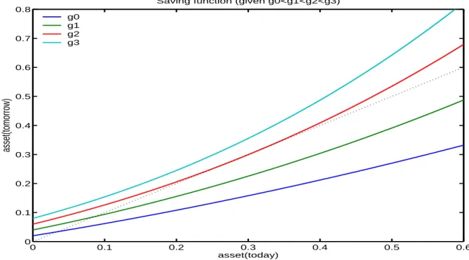
When g > 0, which would be the typical feature of a constrained-efficient steady state, the constrained-efficient savings function looks quite different. This is illustrated in Figure 5. For a given interest rate, this figure plots the savings rule for various levels of g. The form of the saving function is convex and it shifts upward as g increases. This implies that there is a maximum level of g that is consistent with the existence of an upper bound of assets holdings. For values of g above this level, such as g3, there is no such upper bound,
implying that aggregate assets must increase without bound, preventing the existence of a steady state for the constrained-efficient economy.
0 0.1 0.2 0.3 0.4 0.5 0.6 0 0.1 0.2 0.3 0.4 0.5 0.6 0.7 0.8
Saving function (given g0<g1<g2<g3)
asset(today) asset(tomorrow) g0 g1 g2 g3
Figure 5: Planner’s savings function for e3 for different values of g. For g > g2 there is no
steady state.
We now characterize the solution, which involves a nonstationary path for capital. 6.2.1 The solution to the planner’s problem
To solve the planning problem numerically, we need to characterize a whole time path for the wealth distribution. For this, we use similar techniques to those developed in Krusell and Smith (1997) and Krusell and Smith (1998); for details, see the appendix. For simplicity, we consider an initial condition not of complete equality, but rather the steady-state distribution of the market economy. Figure 6 shows the properties of the solution for the initial condition given by the market steady state.
We see increasing capital accumulation toward a steady-state value for capital. This reveals a path with gt> 0.
0 200 400 600 800 1000 4 6 8 10 12 1st moment 0 200 400 600 800 1000 0 2000 4000 6000 8000 2nd moment 0 200 400 600 800 1000 0 1 2 3 4 5 6x 10 6 3rd moment time 0 200 400 600 800 1000 0 1 2 3 4 5 6x 10 9 4th moment time
Figure 6: Transition from the market steady state to the constrained optimum
more and more concentrated over time, as illustrated in Figure 7, which shows the measure of people with zero asset holdings over time.
This measure becomes larger and larger, while the average asset holding stays bounded around 10. Thus, a more and more vanishingly small fraction of the agents hold the bulk of the capital over time, leading to a limit where a measure-zero set of agents holds all the capital.
The origin of the extreme long-run wealth distribution is a form of “increasing returns” to saving of the constrained optimum, as illustrated above in the convex savings rules. The third term in the first-order condition, the constant g, which is an additional marginal benefit from savings, is particularly large in relative terms for rich consumers, whose marginal utilities of
0 50 100 150 200 0 50 100 150 200 250 0 0.2 0.4 0.6 0.8 1 Asset Time
Figure 7: Density function for assets for each period: Aiyagari model
consumption are low: the more you save, the more important is this term for further savings decisions.
7
Conclusion
In this paper we have investigated the welfare properties of the one-sector neoclassic growth model with uninsurable idiosyncratic shocks. We have relied on the constrained efficiency concept used in the general equilibrium literature, and we have demonstrated constrained inefficiency for our model. We have also provided a characterization of constrained efficiency by means of the first-order condition of a planner’s problem that points to the margins of relevance for whether capital is too high or too low in equilibrium: the income composition
of the (consumption-)poor. The mechanism is simple: if the income of the poor comes mainly from labor earnings, ex-ante (constrained-efficient) risk considerations demand that the long-run capital stock be increased, because that raises wages and therefore the income of the poor. We then calibrated our benchmark model parameters governing idiosyncratic risks to the U.S. earnings and wealth distribution, and for this distribution the income of the poor is mainly composed of labor earnings. Using numerical model solution, we then computed the constrained-efficient steady state for our model economy, and we concluded that the long-run capital stock in a laissez-faire world is not only too low, but much too low. We also illustrated how the income composition of the poor matters by looking at alter-native parameterizations, which indeed yield qualitatively different results than we obtained for our benchmark economy. For a parameterization where risk is unemployment risk (thus not properly depicting the actual earnings distribution), the laissez-faire capital stock is too high, because now the poor have no labor income. For the parameterization of earnings in Aiyagari (1994) (which generates too little dispersion in earnings and in wealth), we find that, as in our benchmark economy, laissez-faire capital is too low. In this case, however, the constrained-efficient outcome involves ever-increasing inequality, something we did not find for our benchmark economy. Ever-increasing inequality can be understood from the per-spective of the planner’s first-order condition, which reveals that there is increasing returns of sorts to constrained-efficient individual savings.
Several questions remain open. One concerns the calibration of individual risk. We follow Casta˜neda, D´ıaz-Gim´enez, and R´ıos-Rull (2003) here, but there are alternative ways of explaining the wide dispersion in wealth that we observe in most economies. One relies on preference heterogeneity, for example as pursued in Krusell and Smith (1997) and Krusell and Smith (1998). There, rich consumers are rich to a large extent because they, or their forefathers, were particularly patient and saved; conversely, the poor are poor to a large
extent because they chose to be poor—they chose to consume in the past. The specific modeling there views discount factors as random (and uninsurable), and thus people are all the same ex ante, but with some persistence in discount factors, significant wealth inequality can be generated even from small cross-sectional heterogeneity. From the perspective of the present paper, a model where wealth inequality derives chiefly from persistent shocks to patience might give quite different results than those we obtain here, since they suggest that wealth inequality is not all a result of incomplete risk sharing. In other words, the planner would be more willing to let those who choose to become poor (rich) stay poor (rich). Similarly, other forms of heterogeneity in preferences (such as risk aversion) or in individuals’ abilities or opportunities (e.g., possibly making it harder for some to participate in asset markets than it is for others) would also be valuable to examine from the perspective of constrained efficiency. Ultimately, microeconomic studies hopefully allow us to better distinguish which elements of individual heterogeneity are key and which are not. The present paper takes a somewhat conservative position by not allowing any other heterogeneity than in earnings, but we firmly believe that it is a useful one and a very natural first step. From the perspective of what causes inequality, it is perhaps not conservative enough: it is perhaps too “left-wing”, because it interprets all successes as luck and all failures as bad luck.
Compared to the findings in Aiyagari (1995) and Aiyagari and McGrattan (1995), the conflicting policy implications are apparent. The question is: should capital taxes be positive or negative (raised or lowered)? A precautionary-savings perspective suggests that there is overaccumulation of capital in the laissez-faire economy, and that capital taxation can improve on the allocation. Such a conclusion is a noteworthy one, since it does alter otherwise standard prescriptions (see, e.g., Chamley (1986)) that call for zero long-run capital taxes. Our findings here, based on the same precautionary-savings model but with a different notion of efficiency, indicate that a move back toward zero taxes may be beneficial, and they
actually suggest that a “radical” move back may be called for: the constrained optimum in our economy has a higher capital stock than that of the first-best allocation. Of course, this indication is based on taking a different stand on what is feasible for the planner; we allow some things that are not allowed in Aiyagari (1995) and Aiyagari and McGrattan (1995), and vice versa. A natural next step of the present analysis is to consider more restrictions on how the planner can alter outcomes. For example, it would be interesting to explore nonlinear taxes on wealth that are not allowed to be state-contingent.
It is also instructive to compare our findings to those in Kehoe and Levine (1993), who consider a complete-markets (endowment) economy with limited commitment/constraints on enforcement. They prove, for their economy, that the competitive equilibrium is “condi-tionally efficient”, which in a world with one good coincides with the constrained-efficiency concept from the incomplete-markets literature that we employ here. One could interpret the lack of contingent-claims markets in our two-period economy as simply reflecting a lack of enforcement: agents can save but any additional contracts contingent on idiosyncratic risk would necessarily involve “paying back” in some states of nature, and therefore such contracts are not feasible. The fact that we find constrained inefficiency here should not be surprising, however, because we do have more than one good per period, (capital services, labor, and consumption), and relative price changes make the notion of conditional efficiency not apply. Our economy is thus only one of many examples where conditional efficiency does not imply constrained efficiency.