HAL Id: hal-03144836
https://hal.archives-ouvertes.fr/hal-03144836
Submitted on 17 Feb 2021
HAL is a multi-disciplinary open access
archive for the deposit and dissemination of
sci-entific research documents, whether they are
pub-lished or not. The documents may come from
teaching and research institutions in France or
abroad, or from public or private research centers.
L’archive ouverte pluridisciplinaire HAL, est
destinée au dépôt et à la diffusion de documents
scientifiques de niveau recherche, publiés ou non,
émanant des établissements d’enseignement et de
recherche français ou étrangers, des laboratoires
publics ou privés.
Distance of Hi-GAL sources
P. Mège, D. Russeil, Annie Zavagno, D. Elia, S. Molinari, C. M. Brunt, R.
Butora, L. Cambresy, A. M. Di Giorgio, T. Fenouillet, et al.
To cite this version:
P. Mège, D. Russeil, Annie Zavagno, D. Elia, S. Molinari, et al.. Distance of Hi-GAL sources.
As-tronomy and Astrophysics - A&A, EDP Sciences, 2021, 646, pp.A74. �10.1051/0004-6361/202038956�.
�hal-03144836�
https://doi.org/10.1051/0004-6361/202038956 c P. Mège et al. 2021
Astronomy
&
Astrophysics
Distance of Hi-GAL sources
?
,
??
P. Mège
1, D. Russeil
1, A. Zavagno
1,2, D. Elia
3, S. Molinari
3, C. M. Brunt
4, R. Butora
5, L. Cambresy
6,
A. M. Di Giorgio
3, T. Fenouillet
1, Y. Fukui
7, J. C. Lambert
1, Z. Makai
1,8, M. Merello
9, J. C. Meunier
1,
M. Molinaro
5, C. Moreau
1, S. Pezzuto
3, Y. Poulin
1, E. Schisano
3, and F. Schuller
10,111 Aix Marseille Univ., CNRS, CNES, LAM, Marseille, France e-mail: delphine.russeil@lam.fr
2 Institut Universitaire de France, Paris, France
3 INAF – Istituto di Astrofisica e Planetologia Spaziali (INAF-IAPS), Via del Fosso del Cavaliere n. 100, 00133 Rome, Italy 4 Department of Physics and Astronomy University of Exeter, Exeter, UK
5 INAF – Osservatorio Astronomico di Trieste, Trieste, Italy
6 Observatoire Astronomique de Strasbourg, Université de Strasbourg, CNRS UMR 7550, 11 rue de l’université, 67000 Strasbourg, France
7 Department of Physics, Graduate School of Science, Nagoya University, Furo-cho, Chikusa-ku, Nagoya 464-8602, Japan 8 Department of Physics and Astronomy, West Virginia University, Morgantown, WV 26506, USA
9 Departamento de Astronomía, Universidad de Chile, Casilla 36-D, Santiago, Chile
10 Leibniz-Institut für Astrophysik Potsdam (AIP), An der Sternwarte 16, 14482 Potsdam, Germany 11 Max-Planck-Institut für Radioastronomie, Auf dem Hügel 69, 53121 Bonn, Germany
Received 16 July 2020/ Accepted 28 November 2020
ABSTRACT
Aims.Distances are key to determining the physical properties of sources. In the Galaxy, large (>10 000) homogeneous samples of sources for which distance are available, covering the whole Galactic distance range, are still missing. Here we present a catalog of velocity and distance for a large sample (>100 000) of Hi-GAL compact sources.
Methods.We developed a fully automatic Python package to extract the velocity and determine the distance. To assign a velocity to a Hi-GAL compact source, the code uses all the available spectroscopic data complemented by a morphological analysis. Once the velocity is determined, if no stellar or maser parallax distance is known, the kinematic distance is calculated and the distance ambiguity (for sources located inside the Solar circle) is solved with the H
i
self-absorption method or from distance–extinction data.Results.Among the 150 223 compact sources of the Hi-GAL catalog, we obtained a distance for 124 069 sources for the 5σ catalog (and 128 351 sources for the 3σ catalog), where σ represents the noise level of each molecular spectrum used for the line detections made at 5σ and 3σ to produce the respective catalogs.
Key words. stars: distances – catalogs
1. Introduction
In the Galaxy, studying the early phases of (high-mass) star for-mation requires distance inforfor-mation but often faces problems of high extinction and large distances. The study of star for-mation laws, from small to large scales, is based on distances and this is at the heart of the Galactic plane large-scale sur-veys and high-resolution pointed observation studies. Among these surveys, the Herschel Galactic plane survey Hi-GAL
(Molinari et al. 2010) delivered unprecedented multi-wavelength
(70 µm, 160 µm, 250 µm, 350 µm, and 500 µm) observations of star-formation sites at different spatial scales, namely from core to clump scales (Elia et al. 2017). However, the deriva-tion of general conclusions regarding Galactic star-formaderiva-tion laws requires the determination of distances for a large number of sources.
? Hi-GAL (Herschel infrared Galactic plane Survey) is a Herschel key project. Herschel is an ESA space observatory with science instru-ments provided by European-led Principal Investigator consortia and with important participation from NASA.
?? Full Table 3 and Table E.1 are only available at the CDS via anony-mous ftp to cdsarc.u-strasbg.fr(130.79.128.5) or viahttp: //cdsarc.u-strasbg.fr/viz-bin/cat/J/A+A/646/A74
Many studies have presented results for compact sources in the Galaxy using available molecular data to determine the radial velocity of sources with respect to the local stan-dard of rest (LSR), and then to derive their kinematic dis-tance using a model of the Galactic rotation curve (Russeil
et al. 2011;Ellsworth-Bowers et al. 2015;Wienen et al. 2015;
Whitaker et al. 2017; Zetterlund et al. 2017). Recently, Gaia
(Gaia Collaboration 2000), measuring stellar parallaxes,
revolu-tionized our view of the distribution and distances of sources in our Galaxy (Cantat-Gaudin et al. 2018;Zucker et al. 2019;Yan
et al. 2019;Lallement et al. 2019) but this holds for a limited
volume around the Sun (heliocentric distance up to 3 kpc in the Galactic plane) and for main sequence stars which do not suf-fer from high extinction (up to AV' 3.5). Indeed, several meth-ods could be used to determine the distance of Hi-GAL sources with Gaia data. One can determine the distance to the parental molecular cloud from the line-of-sight extinction, but as under-lined byYan et al.(2019) andLallement et al.(2019) this is lim-ited to extended clouds and to distances up to 3 kpc. One could determine the distance of any associated cluster, but looking at
Cantat-Gaudin & Anders (2020) the mean Bayesian Gaia
dis-tance of the open clusters (with −2◦< b < 2◦) is 2.84 kpc (max-imal distance reached being 9.75 kpc). Finally, one could deter-mine the distance of young stellar objects (YSOs) embedded in
Open Access article,published by EDP Sciences, under the terms of the Creative Commons Attribution License (https://creativecommons.org/licenses/by/4.0),
Hi-GAL sources; this method would be the best. To evaluate this possibility we estimate the distance that can be reached with this method. From a sample of 20 massive Galactic star-forming complexes (d= 0.4–3.6 kpc) studied byPovich et al.(2013), we estimate a median value for YSO extinction of AV= 7.1 (and a mean of AV= 12) then AG= 6 (with AG/AV= 0.859). A 2 Myr PARSEC isochrone (Marigo et al. 2017) gives us a G band abso-lute magnitude of 5 and −1.64 for YSOs of 0.5 M and 8 M , respectively. Knowing that the Gaia-DR2 catalog is complete between G = 12 and G = 17, this means that YSOs of 0.5 M and 8 M can be detected up to 158 pc and 3.4 kpc, respectively (for AV= 7.1). Therefore, Gaia results are insufficient for the study of distant and/or highly embedded sources.
In the framework of the European FP7 SPACE project VIALACTEA1 dedicated to the scientific exploitation of the
Hi-GAL survey, we embarked on the determination of distances for the 150223 compact sources from velocity assignment and kinematic distance determination. Given the large number of sources, this represents an unprecedented effort to deliver reli-able distances to the scientific community, allowing the statisti-cal study of clump physistatisti-cal properties.
This paper is organized as follows: Sect.2presents the sam-ple of Hi-GAL sources and the molecular data used to deter-mine the sources velocity. Section3describes the method used to determine velocity and distance and illustrates the different steps of the process. Results obtained from this work together with comparisons with published results available in the litera-ture are presented in Sect.4. Conclusions are given in Sect.5.
2. Sample and data used
The Herschel infrared survey of the Galactic plane, Hi-GAL
(Molinari et al. 2010), is a complete survey of the Galactic
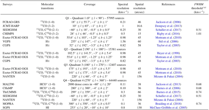
plane performed in five infrared photometric bands centered at 70, 160, 250, 350 and 500 µm. After band merging, 150 223 compact sources have a spectral energy distribution (SED) eli-gible for gray-body fit (Elia et al., in prep.) but lack the dis-tance information needed to evaluate their physical properties. A first version of the catalog is presented inElia et al.(2017) for 100 922 sources located in the inner Galaxy (−71◦ < l < −67◦). Table1list the spectroscopic surveys used to assign radial veloc-ities to the Hi-GAL compact sources. Some surveys cover a large area of the Galactic plane, such as for example the SEDIGISM survey (−60◦ < l < +18◦, |b| < 0.5◦) while some others have a more limited coverage, such as CHIMPS (28◦ < l < 46◦and |b| < 0.5◦). Also, there are some gaps in the coverage of the Galactic plane, such as for sources in the longitude range 195◦– 205◦, for sources with|b| > 0.5◦and 1◦< l < 17◦, and for sources with b > 1.7◦and 66◦< l < 101◦.
3. Distance determination method
The first step in determining the distance is to measure the radial velocity of the GAL sources. Here, because most of the Hi-GAL sources are expected to be associated with dense molecular material, we measure their radial velocities from molecular line observations. Many spectroscopic surveys of the Galactic plane are available and have been used for this work; these are listed in Table1.
To derive the distance of sources in the Milky Way we have to assume that the measured radial velocity (VLSR) with respect
1 FP7-SPACE-2013-1 call with Grant Agreement No. 607380.
to the local standard of rest of the source arises from its dif-ferential Galactic rotation. Subsequently, using a model for the rotation of the Galaxy, one can obtain the kinematic distance to the source from its radial velocity, VLSR. To this end, we adopt the revised Galactic rotation curve presented in Russeil et al.
(2017). The rotation curve models axially symmetric circular orbits, but the true rotation pattern can be more complicated. Indeed velocities can depart from circular rotation, mainly due to streaming motions (Burton 1971;Stark & Brand 1989;Russeil 2003), and then can cause large uncertainty in the derived dis-tances. Typical velocity departures are of about 10 km s−1(e.g.,
Roman-Duval et al. 2009;Anderson et al. 2012;Wienen et al.
2015) but can reach up to 40 km s−1 (Brand & Blitz 1993). In addition, while the procedure of transforming velocities into dis-tances is straightforward in the outer Galaxy, there is the well-known kinematic distance ambiguity (KDA) for sources in the inner Galaxy. Each velocity measurement leads to two possible distances, the near and far distances, which correspond to the two equidistant points from the tangent point (the closest position on the line of sight to the Galactic center). Choosing between the near and far distances is only possible using additional informa-tion, such as for example extinction and H
i
data cubes along the same line of sight (e.g.,Russeil et al. 2011).3.1. Algorithm outline
We developed the Python program starbird to determine the velocity and the distance of Hi-GAL sources. starbird assigns heliocentric radial velocities and distances to sources of the Hi-GAL survey by means of the VIALACTEA Knowledge Base (VLKB, Molinaro et al. 2016). The starbird program has five main steps, as shown on Fig.1.
starbirdaccepts an input table of sources in a specific for-mat. This table contains mandatory information on the sources including a source running number, a source name which here is the Hi-GAL name (as given in the catalog of Elia et al. 2017), the Galactic and equatorial coordinates (in degrees), and the source elliptical footprint information (the major and minor axes full width at half maximum (FWHM) in arc-seconds and position angle (PA) in degrees) measured at 250 µm. starbird executes a series of actions (labeled QUERY, DOWNLOAD, RADIAL, FILTER, MORPHO, SELECT-VLSR, BROWSE and COMPUTE) which are described below.
3.2. Velocity extraction
The first step to finding the source velocity is to download the molecular data cubes and fit the spectra extracted at the position of the source. For a given source, the tasks QUERY and DOWN-LOAD list, query, and download the portion of the observational data cubes available in the VLKB. Depending on the Galactic longitude of the source there can be up to 11 different molecular data cubes available (see Table1).
For all downloaded data cubes, the RADIAL task extracts a single profile at the central position of the source and per-forms a multi-Gaussian fitting. The developed fitting method is described in AppendixA. The FILTER task is then applied on the fitted lines, and is applied in every region of the l−VLSRplane except in kinematic avoidance zones (±20 degrees range around the Galactic center and anti-center direction), because in these regions anomalous streaming motions cause VLSR to strongly depart from the ideal circular motion. It first removes all indi-vidual velocity components that have a post-fit peak intensity with a signal-to-noise ratio (S/N) < 5 for the 5σ catalog and <3
Table 1. Surveys used to assign radial velocities to the Hi-GAL compact sources.
Surveys Molecular Coverage Spectral Spatial References FWHM
transitions resolution resolution threshold(a)
(km s−1) (arcsec) (km s−1)
Q1 – Quadrant 1 (0◦≤ l< 90◦) – 57995 sources
FCRAO-GRS 13CO (1–0) 18◦≤ l ≤ 55.7◦, −1◦≤ b ≤ 1◦ 0.21 46 Jackson et al.(2006)
JCMT-HARP 12CO (3–2) 10◦≤ l ≤ 65◦, −1◦≤ b ≤ 1◦ 1 16.6 Dempsey et al.(2013)
SEDIGISM 13CO, C18O (2–1) −60◦≤ l ≤ 18◦, −0.5◦≤ b ≤ 0.5◦ 0.25 30 Schuller et al.(2017) 0.51
CHIMPS 13CO, C18O (3–2) 28◦≤ l ≤ 46◦, −0.5◦≤ b ≤ 0.5◦ 0.5 15 Rigby et al.(2016) 1.01
Exeter FCRAO OGS 12CO,13CO (1–0) 55.6◦≤ l ≤ 103◦, −1.25◦≤ b ≤ 1.25◦ 0.98 45 Mottram et al.(2010)
VGPS Hi 255◦≤ l ≤ 147◦, −1◦≤ b ≤ 1◦ 1.56 60 Stil et al.(2006)
CGPS Hi 52◦≤ l ≤ 192◦, −3.5◦≤ b ≤ 5.5◦ 0.82 58 Taylor et al.(2003)
Q2 – Quadrant 2 (90◦≤ l< 180◦) – 15381 sources
Exeter FCRAO OGS 12CO,13CO (1–0) 102.5◦≤ l ≤ 141.5◦, −3◦≤ b ≤ 5.4◦ 0.98 45 Heyer et al.(1998)
Exeter FCRAO OGS 12CO,13CO (1–0) 55.6◦≤ l ≤ 103◦, −1.25◦≤ b ≤ 1.25◦ 0.98 45 Mottram et al.(2010)
CGPS Hi 52◦≤ l ≤ 192◦, −3.5◦≤ b ≤ 5.5◦ 0.82 58 Taylor et al.(2003)
Q3 -Quadrant 3 (180◦≤ l< 270◦) – 12407 sources
Exeter FCRAO OGS 12CO,13CO (1–0) 175◦≤ l ≤ 193◦, −3.5◦≤ b ≤ 5.5◦ 0.98 45 Mottram et al.(2010)
Exeter FCRAO OGS 12CO,13CO (1–0) 141◦≤ l ≤ 175◦, −3.5◦≤ b ≤ 5.4◦ 0.98 45 Mottram et al.(2010)
NANTEN 12CO (1–0) 220◦≤ l ≤ 60◦, −5◦≤ b ≤ 5◦ 1 156 Mizuno & Fukui(2004)
Q4 – Quadrant 4 (270◦≤ l< 360◦) – 64440 sources
MALT90 HCO+(1–0) 2000 dense cores in −60◦≤ l ≤ 20◦ 0.11 38 Jackson et al.(2013) 0.68
CHaMP HCO+(1–0) 280◦≤ l ≤ 300◦, −4◦≤ b ≤ 2◦ 0.10 36 Barnes et al.(2006) 0.68
ThrUMMS 12CO,13CO, C18O (1–0) 299◦≤ l ≤ 359◦, −1◦≤ b ≤ 1◦ 0.3 66 Barnes et al.(2015) 0.74
SEDIGISM 13CO, C18O (2–1) −60◦≤ l ≤ 18◦, −0.5◦≤ b ≤ 0.5◦ 0.25 30 Schuller et al.(2017) 0.51
NANTEN 12CO (1–0) 220◦≤ l ≤ 60◦, −5◦≤ b ≤ 5◦ 1 156 Mizuno & Fukui(2004)
MOPRA 12CO,13CO, C18O (1–0) 300◦≤ l ≤ 350◦, −0.5◦≤ b ≤ 0.5◦ 0.1 36 Braiding et al.(2018) 0.74
SGPS HI 253◦≤ l ≤ 20◦, −10◦≤ b ≤ 10◦ 0.8 130 McClure-Griffiths et al.(2005)
Notes.(a)His is the threshold used in the FILTER task to remove spikes. No threshold is applied for surveys without such artefact.
for the 3σ catalog. It then removes spiky features by removing overly narrow lines. This rejection is based on a minimum fit-ted FWHM threshold that depends on the survey (see last col-umn in Table 1 and Appendix A). FILTER also removes the velocities that would lead to a negative rotation frequency and those that are inconsistent with the angular rotation model; the suspected extragalactic velocities (i.e., those that give a galacto-centric distance larger than 17 kpc); the kinematically forbidden VLSR (i.e., those that go beyond the tangent point velocity by more than 20 km s−1); and finally it applies a selection process favoring velocities falling in the l − VLSRmap fromDame et al. (2001).
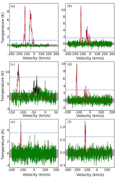
Figure 2 shows an example of fitted spectra for the Hi-GAL source HIGALBM340.2690-0.0542 for which a velocity of −125 km s−1is adopted. On this example we note that the dense-gas tracer lines (Figs.2e and f) allow a reliable and unique ity determination. Because they better probe the clumps veloc-ity and show simpler spectra, dense-gas tracers better determine the velocity of a source. Indeed, for BGPS (Bolocam Galactic Plane Survey) objects,Ellsworth-Bowers et al.(2015) show that for objects with a HCO+(3–2) velocity, 95% have 13CO(1–0) velocities in agreement. In addition, we need that the dense-gas tracer line often corresponds to the most intense line in the lower-density-gas tracer. However, in about 40% of the cases only the low-density-gas tracer, or a single molecular transition spectrum with multiple lines, is available. However, instead of adopting the most intense line velocity directly, we perform a morphological analysis as described in the following section.
3.3. Morphological analysis and velocity assignment
Most of the time the observed spectra show several peaks and then the velocity extraction process returns several velocities. Along the line of sight, the molecular emission can come from a diffuse layer or from a more structured medium such as clumps
and filaments. One way to choose the best velocity is to suppose that the Hi-GAL sources belong to such a structured molecular medium. The MORPHO task has been developed to lead such a morphological analysis. For every fitted velocity, the script auto-matically extracts the plane from the data cube at this velocity and performs a basic source extraction using SExtractor software
(Bertin & Arnouts 1996) to reveal the presence of some elliptical
emission structures. If the molecular emission is diffuse then no source will be found, while if the emission is structured, molec-ular sources will be detected and some of them may intersect the Hi-GAL footprint. For the SExtractor detected sources, their roundness, their center angular distance to the Hi-GAL source center, and their overlapping area and filling factor with the Hi-GAL source are evaluated. A score is then attributed (coded by an integer between 0 and 4) spotting whether there is no over-lapping source, a partial overlap, the source is included in the Hi-GAL one (and vice versa), or a complete overlap, respec-tively. The task SELECT-VSLR then scans all the available information on the fitted lines in order to choose the best line. Regarding the existence of positive scores for the molecular lines, different criteria are used. For each of these lines, an addi-tional condition is applied: the line has to be confirmed by the presence of another line in a different molecular tracer among those available (with a velocity difference of less than 7 km s−1). If no line is confirmed, we choose by default the velocity of the most intense line from the densest available tracer. For con-firmed lines the choice of the velocity is as follows. If lines have a morphological score attached to their velocities (by the previ-ous action MORPHO), the velocity of the highest scoring line is selected. If two or more lines share the best score, the best angular separation (the smallest) is the next criterion. If they also have the same angular separation, the roundness (the highest) is the next criterion. If none of the confirmed lines have a score, we choose the velocity of the most intense line from the confirmed densest molecular tracer lines.
Input table
Hi-GAL compact sources (position, 250 m size)
QUERY & DOWNLOAD Extract molecular data-cubes (VLKB)
RADIAL & FILTER
Fit spectra VLSR extractions & selection
MORPHO
Morphological analysis of molecular emissions & Match with Hi-GAL emission VLSR - morpho. scoring
SELECT_VLSR Final VLSR selection VLSR
COMPUTE
Distance calculation - Resolve KDADistance
Output table
Source position, VLSR , molecular tracer,
Heliocentric and galactocentric distances, labels ...
Fig. 1.Flowchart for velocity determination.
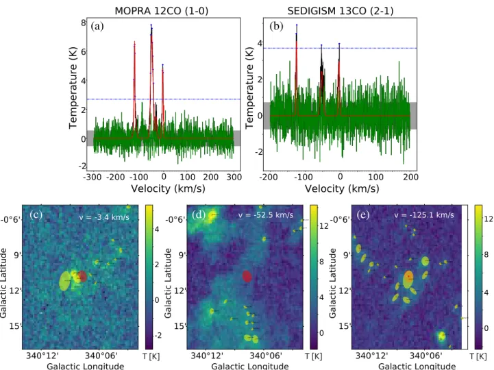
Figure 3 shows an example of the morphological anal-ysis and the velocity assignment performed to the source HIGALBM340.1288-0.1837. For this source two molecular data cubes are available and both extracted spectra are in agree-ment, showing three lines at −3.4 km s−1, −52.5 km s−1, and −125.1 km s−1 but with different relative intensity. In MOPRA 12CO(1–0), the highest peak is for the −52 km s−1 while in SEDIGISM13CO(2–1) this is the −125.1 km s−1. This could be due to an optical thickness effect knowing that the 12CO(1–0) emission usually comes from the cloud surface and/or a more diffuse medium. Thanks to the morphology analysis we can see that a structured source is found towards the Hi-GAL source (clear overlapping of the footprints) only at −125.1 km s−1 (Fig.3e) which leads us to assign this velocity to the source. This also confirms that the −52.5 km s−1 velocity component corre-sponds to more-diffuse emission as illustrated in Fig.3d. 3.4. Distance determination: solving the kinematic distance
ambiguity
The distance determination is performed by the task COMPUTE. The distance of a source can be derived either from kinematics or in a more direct way (stellar distance of the associated H
ii
region or maser parallax distance). For the kinematic distance calculation, theReid et al.(2009) fortran code was used but with the revised rotation curve adopted for the VIALACTEA project(Russeil et al. 2017).
When the VLSR of a source is assigned, the kinematic dis-tance (dkin) can be calculated. At this step, three scenarios must
-300 -200-100 0 100 200 300 0 2 4 6 8 T e m p e ra tu re ( K ) -2 0 2 4 6 8 10 0 5 10 Velocity (km/s) -2 0 2 4 -0.5 0.0 0.5 1.0 (a) (b) (c) (d) (e) (f) -5 10 0 2 4 -2 6 8 T e m p e ra tu re ( K ) T e m p e ra tu re ( K ) Velocity (km/s) 200 300 100 0 -100 -200 -300 200 100 0 -100 -200 100 0 0 100 200 -100 -100 -200 -200 0 -100 -150 -50 50 -300 Velocity (km/s) Velocity (km/s) Velocity (km/s) Velocity (km/s)
Fig. 2.Example of fitted molecular spectra for VLSR detection for the Hi-GAL source HIGALBM340.2690-0.0542. The spectra are (a) NAN-TEN12CO(1–0), (b) MOPRA 12CO(1–0), (c) TRUMMS12CO(1–0), (d) SEDIGISM13CO(2–1), (e) SEDIGISM C18O(2–1), (f ) MALT90 HCO+. In all panels the black, red, and green curves are the extracted profile, the fitted lines, and the residual, respectively. The background gray area is the ±σnoisevalue where σnoiseis the root mean squared value of the noise amplitude (see AppendixA). The horizontal blue line shows the 5σ level.
be considered: (1) the source is outside the solar circle and there-fore dkin is unique; (2) the source lies inside the Solar circle but its velocity is forbidden, hence the tangent point distance is adopted; (3) the source lies inside the Solar circle with a valid velocity, and therefore two distances are possible and the kinematic distance ambiguity (KDA) must be solved to choose between the far distance, dFAR, and the near distance, dNEAR.
To solve the KDA, or to directly adopt a stellar or maser par-allax distance, the task first cross-correlates (both spatially and in velocity, when possible) the source with available published cat-alogs (listed in the note of Table2) in which the KDA is already solved, or giving us sufficient information to solve it or to assign a stellar or maser parallax distance.
Because Hi-GAL sources located in quadrants Q2 and Q3 are not affected by any KDA, their distance is directly assigned from their known radial velocity. For the Hi-GAL sources located in Q1 and Q4, the near/far distance ambiguity is resolved going down through the list of methods arranged in order of prior-ity (see priorprior-ity order in Table2). The methods used to decide
-300 -200 -100 0 100 200 300 -2 0 2 4 6 8 T e m p e ra tu re ( K )
MOPRA 12CO (1-0) SEDIGISM 13CO (2-1)
Velocity (km/s) clump #1 clump #2 clump #3 clump #4 clump #5 clump #6 clump #7 clump #8 clump #9 clump #10 clump #11 v = -3.4 km/s 340°12' -0°6' 9' 12' 15' Galactic Longitude G a la ct ic L a ti tu d e 4 clump #1 clump #2 clump #3 clump #4 clump #5 clump #6 clump #7 clump #8 clump #9 clump #10 clump #11 clump #12 clump #13 clump #14 clump #15 clump #16 clump #17 v = -52.5 km/s 0 4 8 12 clump #1 clump #2 clump #3 clump #4 clump #5 clump #6 clump #7 clump #8 clump #9 clump #10 clump #11 clump #12 clump #13 clump #14 clump #15 clump #16 clump #17 clump #18 clump #19 clump #20 clump #21 clump #22 clump #23 clump #24 clump #25 v = -125.1 km/s
(a)
(b)
(c)
(d)
(e)
Velocity (km/s) G a la ct ic L a ti tu d e G a la ct ic L a ti tu d e Galactic Longitude Galactic Longitude T e m p e ra tu re ( K ) T [K] 0 100 200 -100 -200 0 2 4 -2 T [K] T [K] 15' 15' 12' 12' 9' 9' -0°6' -0°6' 340°06' 340°12' 340°06' 340°12' 340°06' 0 2 -2 12 8 4 0Fig. 3.Example of the morphological analysis of the molecular emission for the Hi-GAL source HIGALBM340.1288-0.1837. The upper panels show the MOPRA12CO(1–0) (a) and SEDIGISM13CO(2–1) (b) fitted spectra. The labels in these panels are the same as in Fig.2. The lower panelsshow the channel maps at −3.4 km s−1(c), −52.5 km s−1(d), and −125.1 km s−1(e). The red ellipse is the footprint of the Hi-GAL source while the yellow ellipses are the footprints of the structures extracted by SExtractor.
whether the source concerned by KDA is located at the near or far distance (dNEARor dFAR) are summarized in Table2.
For example, because infrared-dark clouds (IRDCs) are cold and dense molecular clouds seen as extinction features against the bright Galactic background, if a source can be associated to an IRDC the near distance will be favored. If a source can be associated to an optical H
ii
region or to a region with a maser parallax then the stellar distance of the Hii
region (or the near distance) or the parallax distance will be adopted. Following the Hi
absorption/emission method (e.g., Anderson& Bania 2009), when a source can be assigned to a radio
H
ii
region for which H2CO or Hi
line of sight absorption lines are observed with absolute velocity larger than the source VLSR then the far distance will be adopted. However, as many sources have no such information, we develop automatic scripts to perform Hi
self-absorption (HISA) and extinction curve analysis.By default, the source is placed at the far distance but if a HISA feature is found at the source VLSR or if an extinc-tion feature is found close to the near distance then dNEAR is adopted. The HISA is illustrated here for the source HIGAL BM329.2039+0.7101 (Fig.4). The script automatically identi-fies all the significant (S/N larger than 3) and regular dips in the HI spectrum (see Appendix B). If a dip is found at the same velocity (within a 3 km s−1 tolerance) as the source VLSR, as is the case here, then dNEARis adopted.
The extinction cubes are fromMarshall et al.(2006)2. They
give AKs value in the form of “l, b, distance” data cubes. The extinction profile (AKs vs. distance along the line of sight) at the central position of the source is extracted, and then the extinc-tion layers along the line of sight are identified from the jump they induce in the extinction profile. As these jumps are eas-ier to identify on the three-order derivative, the script automati-cally identifies them as minima deeper than 3σ from the baseline level. The extinction analysis is illustrated here for the source HIGALBM1.7647-0.4806 (Fig. 5) for which dFAR= 13.04 kpc and dNEAR= 3.63 kpc, respectively. In our example, one extinction layer at 3.7 kpc is identified, favoring the near dis-tance. We therefore adopt dNEAR= 3.63 kpc for this source.
A last option used to distinguish between dFARand dNEAR is to follow the method used bySolomon et al.(1987). This method considers the physical distance of the source to the Galactic plane: if by taking the far distance the cloud is too far from the Galactic plane (i.e., >140 pc, which is the scale height of the gaseous disk of the Galaxy) then the near distance will be favored. We note that because the sources with KDA are located within the Solar circle, this criterion is not affected by the Galac-tic warp which starts outside the Solar circle.
2 In practice an updated version of the cubes is used (Marshall et al., in prep.).
Table 2. Methods used for distance disambiguation with their associated priority codes.
Priority order Code Method used for disambiguation
1 MDIST Maser distance(a)
2 SDIST_GROUP Stellar distance from grouping (optical H
ii
regions, literature(b))3 SDIST_EXT Kinematic distance from spectral abs. line (literature(c))
4 KDIST_GROUP Kinematic distance from grouping (radio HII regions, literature(b))
5 KDIST_IRDC Kinematic distance from IRDC/dark clouds (literature(d))
6 KDIST Kinematic distance from daughter clouds (for Q1 only, Brunt et al.(e))
7 CLOUD_EXT Kinematic distance from Extinction datacubes
8 HISA_DIST Kinematic distance from HI profile self-absorption analysis
9 SOLO_DIST Kinematic distance from Solomon( f )method (distance above the galactic plane)
— NO_KDA No solution (hence far distance adopted)
— KDA_NO No velocity (hence velocity= −999.)
— NO_AMB No kinematic ambiguity
— TGT_POINT Tangent point distance (forbidden velocity)
References.(a)Reid et al.(2009,2014),Wu et al.(2014),Honma et al.(2012),Bobylev & Bajkova(2013);(b)Russeil(1998);(c)Wienen et al. (2015),Anderson et al.(2015),Urquhart et al.(2012),Anderson & Bania(2009),Roman-Duval et al.(2009),Busfield et al.(2006),Sewilo et al.
(2004),Watson et al.(2003),Kolpak et al.(2003),Pandian et al.(2008),Araya et al.(2002);(d)Chira et al.(2013),Liu et al.(2013),Peretto &
Fuller(2009),Jackson et al.(2008),Du & Yang(2008),Simon et al.(2006a,b),Otrupcek et al.(2000);(e)Brunt et al. (in prep.) Position-position-velocity dendrogram analysis has been applied to the NANTEN datacube. Then, when possible the maser or stellar distance or the near/far choice is assigned to the identified structures.( f )Solomon et al.(1987).
-200 -150 -100 -50 0 50 100 150 vlsr [km/s] 0 20 40 60 80 100 120 T [ K ]
Fig. 4. Example of HISA identification for the source HIGALBM329.2039+0.7101 with assigned VLSR= −63.562 km s−1. The H
i
profile is plotted in blue, and the identified dips are shown as red dots. The horizontal gray thick line shows the ±σnoiseand the dashed red line shows the 3σnoiselevel. The black vertical dashed line and the gray shadow are the velocity of the source and the 3 km s−1 tolerance.The distance determination script tests the different methods in a hierarchical way following the priority list given in Table2. At the beginning, the source is placed at the far distance, and then this distance is changed if one of the listed conditions is fulfilled. Usually the choice of the distance is validated by only one method (which is indicated as the “STATUS” in the final table), but because all the methods are tested, the number of validated methods is coded in the final table as the “PROBA” number; the higher this number, the more reliable the distance decision. 0.0 0.5 1.0 1.5 2.0 AK
Smoothed extinction curve
0.0 0.2 0.4 0.6 0.8 AK /kp c
Smoothed 1st-order derivative
1.0 0.5 0.0 0.5 1.0 AK /kp c
Smoothed 2nd-order derivative
2 4 6 8 10 12 14 Heliocentric distance (kpc) 5 0 5 AK /kp c 3
Smoothed 3rd-order Derivative
Source id = 832720 Extinction analysis (K-band) @ (l,b)=(1.765,-0.481)
2
Fig. 5. Example of extinction layer identification for the source HIGALBM1.7647-0.4806. The detection used the third derivative of the extinction curve. Here, one extinction layer is identified (red dot and dashed line) at a distance of 3.7 kpc.
4. Results
Results are presented in Table 3 (the complete table is avail-able at CDS and the 3σ version of the tavail-able is also deliv-ered as described in Appendix E). The columns are as fol-lows: Col. 1: Hi-GAL source name; Cols. 2–5: equatorial and Galactic coordinates; Cols. 6 and 7: adopted velocity and its uncertainty; Col. 8: molecular tracer used for the veloc-ity determination; Cols. 9 and 10: assigned distance and its uncertainty; Col. 11: method used for the distance determina-tion as listed in Table2; Col. 12: probability that the source has the assigned distance (this is a simple evaluation of the num-ber of different methods assigning the chosen distance, e.g., PROBA= 0.22 means that two methods over the nine agree with the adopted distance assignment); Cols. 13–18: far and
near kinematic distances and their upper and lower uncertain-ties (without any correction applied); Col. 19: the galactocentric distance; and Col. 20: detected extinction features listed as dis-tance, AKs pairs.
One problem that arises when determining the kinematic dis-tances in the Galaxy is that the arm perturbation can introduce radial and azimuthal gas streaming motions (e.g.,Roberts 1969;
Englmaier 2000; Ramón-Fox & Bonnell 2018). Such
stream-ing motions are taken into account in the determination of the distance uncertainty by assuming a typical velocity dispersion of 7 km s−1, but when the streaming motion induces a system-atic and larger velocity shift, as is the case in the Perseus arm between l = 90◦ and l = 160◦ (e.g.,Roberts 1972;Georgelin
& Georgelin 1976;Brand & Blitz 1993) we must add a velocity
correction. We then first delineate the Perseus arm by determin-ing the arm velocity range (only between l = 90◦ to l= 160◦) from the 12CO longitude-velocity plot ofDame et al. (2001). We then select HiGAL sources in these velocity and longitude ranges and apply to these sources (4405 sources with a kine-matic distance) a correction of 14.9 km s−1(Russeil et al. 2007) to the measured VLSR before re-calculating the kinematic dis-tance. This correction is illustrated in Fig.6.
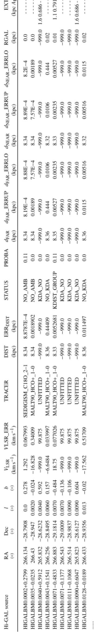
Figure 7 shows the distribution of sources with deter-mined radial velocities. We are able to assign a velocity for 124 069 sources (82.6%). We can split the sample of sources with no velocity assignment into sources that are not covered by any molecular surveys (57.4%) and sources for which the extracted spectrum is too noisy to perform any line fitting or to obtain a fitted line above a 5σ threshold (42.6%). For the first group of sources, we clearly identify the two gaps in the lon-gitude coverage (around l = 190◦ and l = 270◦) and latitude coverage limitation of the survey for some part of Q1 and Q2. For the second group of sources we note that 19% of them have a velocity if the fitted line intensity threshold is lowered to 3σ (instead of 5σ).
Figure 8 shows a zoom (−60◦ < l < 60◦) on the long-itude–velocity distribution of all Hi-GAL sources for which we obtained a velocity (124069 sources). The gray-scale image shows the distribution of the molecular gas traced by the inte-grated 12CO emission fromDame et al. (2001). We note that the sources closely follow the large-scale prominent molecular features.
Urquhart et al. (2018) derived the physical properties of
approximately 8000 ATLASGAL clumps (located in quadrants 4 and 1). To do so, they first assigned radial velocities to the clumps and used a series of criteria (see their Fig. 5 with the flow chart) to determine distances for the clumps. In order to compare our results with their velocity and distance determi-nations, we first cross-correlated the ATLASGAL and Hi-GAL compact-source catalogs with a radius of 1400 for the cone search. ATLASGAL and Hi-GAL sources are paired on the basis of their physical proximity. Due to the maximum radius of 1400and differences in ATLASGAL and Hi-GAL survey cov-erage, the number of paired sources is 6268. Among them, 5976 sources have velocity in both surveys.
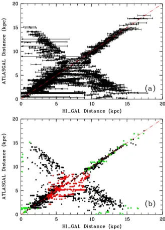
Figure9shows the comparison of velocity determination for paired ATLASGAL and Hi-GAL sources. The colors code the separation between the sources. We note that the source scatter-ing around the one-to-one line is not due to mismatchscatter-ing. We find that 89.4% and 91.8% of the sources have a velocity di ffer-ence smaller than 5 km s−1and 10 km s−1, respectively.
To make a comparison of distance determinations for paired sources, and in particular to compare the KDA solution, we must select sources with similar velocity. We then select sources with velocity difference smaller than 5 km s−1. In addition, we
keep sources with longitude outside ±12◦ around the center Table
3. V elocity and distance for the Hi-GAL compact sources Hi-GAL source RA Dec l b VLSR V LSR_ERR TRA CER DIST ERR DIST ST A TUS PR OB A dFAR dFAR _ERR UP dFAR _ERRLO dNEAR dNEAR _ERR UP dNEAR _ERRLO RGAL EXT (◦ ) (◦ ) (◦ ) (◦ ) (km s − 1) (km s − 1) (kpc) (kpc) (kpc) (kpc) (kpc) (kpc) (kpc) (kpc) (kpc) (kpc AK s ) HIGALBM0.0002 + 0.2799 266.134 − 28.7908 0.0 0.278 1.292 0.067993 SEDIGISM_C18O_2–1 8.34 8.8787E − 4 NO_AMB 0.11 8.34 8.19E − 4 8.88E − 4 8.34 8.89E − 4 8.2E − 4 0.0 -HIGALBM0.0035 − 0.0235 266.43 − 28.947 0.0020 − 0.024 − 16.828 0.34009 MAL T90_HCO + _1–0 8.34 0.0018902 NO_AMB 0.0 8.34 0.00189 7.57E − 4 8.34 7.57E − 4 0.00189 0.0 -HIGALBM0.0040 + 0.5912 265.832 − 28.6232 0.0040 0.592 − 999.0 99.875 UNFITTED − 999.0 − 999.0 KD A_NO 0.0 − 999.0 − 999.0 − 999.0 − 999.0 − 999.0 − 999.0 − 999.0 1.6 0.686 -HIGALBM0.0043 + 0.1541 266.256 − 28.8495 0.0060 0.157 − 6.6484 0.033997 MAL T90_HCO + _1–0 8.36 0.44409 NO_KD A 0.0 8.36 0.444 0.0106 8.32 0.0106 0.444 0.02 -HIGALBM0.0071 − 0.4833 266.883 − 29.1814 0.0070 − 0.484 18.75 0.077026 MAL T90_HCO + _1–0 8.33 0.0052681 KDIST_GR OUP 0.11 8.35 0.00527 0.00235 8.33 0.00235 0.00527 0.01 1.1 0.791 -HIGALBM0.0071 − 0.1377 266.543 − 29.0009 0.0070 − 0.136 − 999.0 99.875 UNFITTED − 999.0 − 999.0 KD A_NO 0.0 − 999.0 − 999.0 − 999.0 − 999.0 − 999.0 − 999.0 − 999.0 -HIGALBM0.0111 − 0.1068 266.514 − 28.9837 0.0090 − 0.106 − 999.0 99.875 UNFITTED − 999.0 − 999.0 KD A_NO 0.0 − 999.0 − 999.0 − 999.0 − 999.0 − 999.0 − 999.0 − 999.0 -HIGALBM0.0090 + 0.6047 265.823 − 28.6127 0.0090 0.604 − 999.0 99.875 UNFITTED − 999.0 − 999.0 KD A_NO 0.0 − 999.0 − 999.0 − 999.0 − 999.0 − 999.0 − 999.0 − 999.0 1.6 0.686 -HIGALBM0.0128 − 0.0189 266.433 − 28.9356 0.013 − 0.02 − 17.562 0.51709 MAL T90_HCO + _1–0 8.36 0.011497 NO_KD A 0.0 8.36 0.0115 0.00516 8.32 0.00516 0.0115 0.02 -... Notes. The full table is av ailable in electronic form at CDS. The full table is also made av ailable for queries within the VLKB catalogs content, also in combination with the other VLKB resources, and deplo yed as an IV O A data collection with IV OID ivo://ia2.inaf.it/vlkb/distances serv ed by the VLKB public T AP service re gistered itself as a V O resource with IV OID ivo://ia2.inaf.it/vlkb/tap .
90 95 100 105 110 115 120 125 130 135 140 145 150 155 160 Galactic longitude (±) 0 1 2 3 4 5 6 7 8 D is ta n c e (k p c )
Fig. 6.Longitude–distance plot in the range of the Perseus arm streaming motion correction (l= 90◦
and l= 160◦
). Blue and red symbols are the source distance before and after the correction. Sources that draw horizontal alignment are sources with the same stellar distance assignation.
0 20 40 60 80 100 120 140 160 180 200 220 240 260 280 300 320 340 360 Galactic longitude (±) ¡2 ¡1 0 1 2 G a la c ti c la ti tu d e ( ±) 0 20 40 60 80 100 120 140 160 180 200 220 240 260 280 300 320 340 360 Galactic longitude (±) ¡2 ¡1 0 1 2 G a la c ti c la ti tu d e ( ±)
Q1
Q2
Q3
Q4
(a)
Q1
Q2
Q3
Q4
(b)
Article number, page 1 of 1
Fig. 7.Spatial distribution of Hi-GAL sources with determined radial velocities (a). Panel b: Hi-GAL sources superimposed with no assigned velocity. Sources not covered by any molecular surveys are shown in red and sources with no line fitted from an overly noisy extracted molecular spectrum are shown in blue. The vertical lines separate the different Galactic plane quadrants (Q1, Q2, Q3 and Q4).
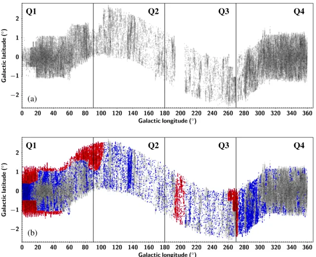
and anticenter directions (because their distance determination is highly uncertain which is due to noncircular motion in the bar or the perpendicularity of the circular motion to the line of sight), and we exclude ATLASGAL sources labeled as “ambigu-ous” and Hi-GAL sources labeled “NO_KDA”. Figure10shows the comparison of distance determinations for this sample (3528 sources). In Fig. 10a, apart from the sources distributed
around the equality line, we observe the classical behavior of anti-correlated distances, which is due to the differences in the distance disambiguation, that is, difference in assignation for a given source between the near and far distance (see Sect.3.4). This is observed for any sources catalog, as illustrated in Fig.C.1
comparing ATLASGAL and BGPS (Ellsworth-Bowers et al. 2015) catalogs. Selecting the ATLASGAL sources for which the
Longitude (
◦
)
V
LS
R
(km
/s)
Article number ,page 1 of 1Fig. 8.Longitude–velocity distribution of all Hi-GAL sources in the range −60◦< l < 60◦
for which we have obtained a velocity. The gray-scale image shows the distribution of the molecular gas traced by the integrated12CO emission fromDame et al.(2001).
100 50 0 50 100 150 VLSR HI_GAL 100 50 0 50 100 150 VLSR ATLASGAL Velocity Comparison 2 4 6 8 10 12 separation - arcsec
Fig. 9.Comparison between paired ATLASGAL and Hi-GAL source velocity. The separation of the sources (in arcsec) is coded in color.
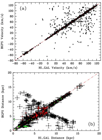
KDA distance has been specifically solved (Flags (iv) to (viii)) we find that 29.5% of the sources disagree for the KDA solution adopted. Nevertheless, we find that 2248 sources (64%) have a distance difference of less than 0.7 kpc (0.7 kpc being the typ-ical distance uncertainty value for the paired Hi-GAL sources) with a mean value of 0.21 kpc. To better understand the distance difference between ATLASGAL and Hi-GAL sources we iden-tify in Fig.10b the sources with the tangent distance choice and sources with velocity lower than 10 km s−1, which are nearby sources (for which the velocity is more representative of any local motions) or sources close to the Solar circle (for which any particular motions produce inaccurate kinematic distances). We performed the same selection and the same comparison (see Fig. 11) with the BGPS catalog (Ellsworth-Bowers et al. 2015) which probes mainly quadrants 1 and 2. The number of paired sources with velocity is 2242, among which 89.2% (2000 sources) have velocity in agreement (∆v ≤ 5 km s−1). From this subsample of sources, we discard those with an uncon-strained KDA solution in both surveys. This leaves us with 799 sources among which 64% (510 sources) have a distance differ-ence of less than 0.5 kpc (which is the typical distance uncer-tainty value for the paired Hi-GAL sources) with a mean value of 0.16 kpc. In addition, selecting the BGPS sources for which the KDA distance has been specifically solved (Flag N or F) we find
Fig. 10.Distance comparison between paired ATLASGAL and Hi-GAL sources (3528 sources). (a) Sources with velocity difference less than 5 km s−1and longitude outside ±12◦
around the center and anti center directions. (b) Same figure but identifying the sources placed at the tan-gent distance in ATLASGAL (in red), and the sources with velocity lower than 10 km s−1(in green). The red dash-dotted line is the y = x line.
that 29.6% of the sources disagree for the KDA solution adopted; a proportion similar to that found for the ATLASGAL compari-son.
Zucker et al. (2020) present a method that combines
Fig. 11.(a) Velocity (2285 sources) and (b) distance (2050 sources) comparison between paired BGPS and Hi-GAL sources. The red dash-dotted line is the y= x line. Same color coding as in Fig.10.
Bayesian framework to infer the distances of nearby dust clouds to a typical accuracy of ∼5%. These latter authors derived a cat-alog of distances to molecular clouds presented in the Handbook of Star Formation, Volumes I (Reipurth 2008a) and II (Reipurth
2008b). To compare our distance results with those ofZucker
et al.(2020) we select the regions that are covered by Hi-GAL
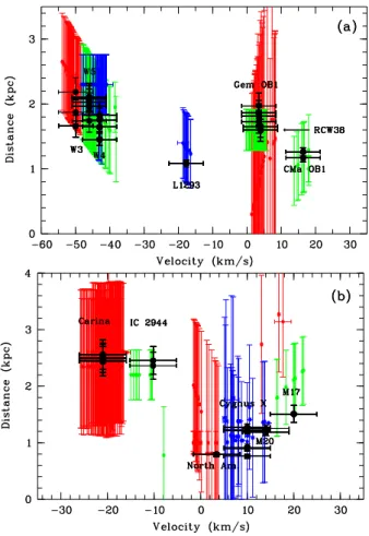
in their list. There are 13 regions common to both our list and that ofZucker et al.(2020), namely CMaOB1, Carina, Cygnus X, GemOB1, IC 2944, L1293, M20, M17, North America, RCW38, W3, W4, and W5. We then select the Hi-GAL sources located at the positions of each region as listed byZucker et al.(2020) and in a similar area (0.2◦) but within ±5 km s−1around the sys-temic velocity of the region. For most of the region the adopted velocity is the H
ii
region VLSR, but for CMaOB1, GemOB1, and IC 2944 the adopted velocity is the VLSRcalculated from the mean radial velocity of the stars (Mel’Nik & Dambis 2009;Sepúlvedaet al. 2011) and for L1293 it is the molecular velocity (Conrad
et al. 2017). We then split the sample into regions located in
quadrants 2 and 3 (then with no KDA) and in quadrants 1 and 4 (with KDA) and display them in Fig.12, a velocity–distance plot (see also Fig. D.1). From Fig. 12 we find a good agree-ment for regions W3, W4, W5, RCW38, Carina, and CMaOB1, an agreement within the error bars for GemOB1, Cygnus X, North America, IC 2944, and L1293, a shift for M17, and a strong dis-agreement for M20. For M20 and GemOB1, their longitude plac-ing them close to the Galactic center and anti-center directions, respectively, leads to an unreliable kinematic distance. Similarly, for North-America, although a few sources agree, others are at the adopted stellar distance while several are too far but can be explained by their longitude being near l = 90◦, a location where the kinematic distance is also uncertain mainly because
of the small value of the velocity in this region. In W5, many sources have been placed at the stellar distance which is slightly farther than theZucker et al.(2020) distance but in agreement with the 2.3 kpc distance found for W3 and W5 byChen et al.
(2020). The most surprising is the disagreement found for M20 and M17. For these two regions, 10 among 13 and 10 among 19 Hi-GAL sources, respectively, have been placed at the far dis-tance (not plotted in Fig. 12). However, for M17 the OB star distance is 2.1 kpc (Hoffmeister et al. 2008), in agreement with our data. This could suggest that the cloud detected byZucker
et al.(2020) is in front of M17 or its distance is underestimated.
We note thatChen et al.(2020) find distances between 1.6 and 1.8 kpc for clouds in the neighborhood of M17. We can invoke the same explanation for M20, as Marshall et al. (2009) and
Schultheis et al.(2014) estimated a distance greater than 4 kpc
for dark clouds and extinction features in the direction and in the neighborhood of the H
ii
region whileTapia et al.(2018) re-evaluate the M20 distance to 2 kpc.Comparison with results presented in Zucker et al. (2020) allows us to illustrate the fact that when studying a particu-lar region it is better to associate the region and the Hi-GAL sources from their velocities and only then to adopt the same dis-tance calculated from the mean or representative velocity of the region. Indeed a small difference in velocity (due e.g., to internal motion) could lead to a large difference in distance.
We must keep in mind that the comparison presented here is done on small areas and in lines of sight that are not always pointing directly toward the considered H
ii
regions. To avoid this, we illustrate the Hi-GAL sources association with a typi-cal star forming region, the W3–W4 Hii
regions complex, for a larger view. We select all the Hi-GAL sources located in the (l, b) coverage of the region and plot these sources in (l, b, v) and (l, b, D) diagrams, v and D representing the velocity and distance obtained from this work. Results are presented for the W3–W4 regions. Figure13shows the Herschel PACS 160 µm image of the W3–W4 Galactic star forming regions together with the 1544 Hi-GAL sources overlaid as points, color-coded according to the velocity-range to which they belong. The asso-ciated sources (858 sources, shown in green) have velocities in the range [−55, −40] km s−1which corresponds to velocities observed for the ionized and molecular gas in these regions. Unfitted sources are coded in blue (422 sources) and sources with velocities out of the [−55, −40] km s−1 range are coded in red (264 sources). Of the 1122 sources with velocity informa-tion, 858 (76.5%) are seen in the range −55 to −40 km s−1.From Fig.13it is clear that knowledge of velocity (and dis-tance) is key to studying star formation. We note that the blue unfitted sources represent an important number of sources. Dedi-cated studies can be envisioned to obtain molecular data for these sources and ascertain their velocity and distance.
Figure 14 shows the (l, b, D) 3D diagram for the regions. Over the 1544 sources (with 422 unfitted, therefore a total of 1122 sources), 478 (43%) are observed in the 1.8–2.3 kpc range, the range obtained byZucker et al.(2020) using Gaia data for the W3–W4 regions (see alsoNavarete et al. 2019for W3). The remaining 644 sources (57%) are observed out of this distance range.
Figure 15 shows the velocity versus distance plot for the W3–W4 regions. The 1544 Hi-GAL sources are represented together with the selected velocity range (−55 to −40 km s−1) in green and the selected distance range (1.8–2.3 kpc) in red. We see that, within the velocity range [−35, 0] and [−90, −60], sources follow the relation between velocity and distance given by the kinematic distance derivation. A similar relation is observed within −35 to −60 km s−1 where the velocity correc-tion has been applied to take into account streaming mocorrec-tions
Fig. 12. Velocity–distance plot of Hi-GAL sources in regions from
Zucker et al.(2020) for sources in quadrants 1 and 2 (a) and in quad-rants 2 and 4 (b), respectively. The velocity (±5 km s−1) and the distance (and its uncertainty) of the sight lines as listed inZucker et al.(2020) are plotted in black. In panel a the Hi-GAL sources are plotted in red (for W3 and GemOB1), blue (for W5 and L1293), and green (for W5, CMaOB1 and RCW38). In panel b the Hi-GAL sources are plotted in red (for Carina, North America, and M20), blue (for Cygnus X), and green (for IC 2944 and M17).
135.5◦ 135.0◦ 134.5◦ 134.0◦ 133.5◦ 2.0◦ 1.5◦ 1.0◦ 0.5◦ 0.0◦ Galactic Longitude (°) Galactic Latitude (° ) W3 - W4 Herschel PACS 160 µm -55 < v < - 40 Unfitted Others
Fig. 13. HerschelPACS 160 µm image of the W3–W4 Galactic star forming regions. The Hi-GAL sources are overlaid as points, color-coded by their velocity: green for sources in the −55 to −40 km s−1 range, blue for unfitted sources, and red for the others with velocities outside the [−55, −40] velocity range.
Galactic longitude (°)
132
133
134
135
136
137
Galactic latitude (°)
0.5
0.0
0.5
1.0
1.5
2.0
D (kpc)
0.0
0.5
1.0
1.5
2.0
2.5
3.0
W3-W4 (l,b,D)
Fig. 14.Three-dimensional (l, b, D) diagram for the W3–W4 regions. 478 (43%) sources are observed in the range 1.8–2.3 kpc, the range of distances obtained byZucker et al.(2020) for these two star forming regions. The color coding is the same as in Fig.13, that is, sources in the range 1.8–2.3 kpc are coded in green, sources outside this range are coded in red, and unfitted sources (with no distance information) are coded in blue; the distance layer for these latter sources is put arbitrarily at 3 kpc for clarity in the plot.
90 80 70 60 50 40 30 20 10 0 v (km/s) 0 1 2 3 4 5 6 7 8 9 D ( kp c) W3-W4 D versus v
Fig. 15.Velocity vs. distance for the W3–W4 regions. The 1544 Hi-GAL sources are represented together with the selected velocity range (−55 to −40 km s−1) in green and the selected distance range (1.8– 2.3 kpc) in red.
observed in this region of the Galaxy. We clearly see the cor-respondence between the velocity range and the distance range, visually explaining how a lower number of sources are found in the corresponding selected distance range (1.8–2.3 kpc) when compared to the number of sources found in the selected velocity range.
In all cases studied, we note that about 50% of the Hi-GAL sources detected in a given region are in the D layer associated with a given molecular star forming cloud. We also note the pos-sibility that for some unfitted sources (hence with no velocity or distance information), when a clear spatial association of the source can be ascertained with complementary information (e.g., near-infrared images), that this spatial association could be used to assign the source to a given molecular star forming region. We recommend users take a careful look at an infrared 2D image of the region, the (l, b, v) and (l, b, D) diagrams, when working on specific regions.
5. Conclusions
In an unprecedented effort to deliver reliable velocity and dis-tance information for a large number of Hi-GAL sources, we developed the Python program starbird, which enables the deter-mination and the assignation of velocity and distance to the Hi-GAL compact sources. We obtained a distance for 124 069 compact sources (among 150 223 sources) of the Hi-GAL cata-log for the 5σ level (and 128 351 sources for the 3σ level). This is the first time that this information has been determined for such a large number of compact sources in a homogeneous way. This Hi-GAL compact source catalog with distance determina-tion constitutes an invaluable resource for studies related to star formation in the Galaxy and Galaxy structure.
A comparison of our results with published velocities and distances coming from ATLASGAL and BGPS surveys shows that the velocity assignment is effective (with typically 89.3% of the sources with a velocity difference of less than 5 km s−1), and the resolution of the KDA disagrees in only 29.6% of the cases. The comparison with nearby regions fromZucker et al.(2020) illustrates that the cataloged distances can be used statistically to lead studies at the scale of the Galaxy. When studying a partic-ular region, we recommend comparing the velocity and spatial distribution of the Hi-GAL sources with the systemic velocity of the region and its morphology, respectively. Finally, a path to improvement will be to update the distance (up to 4 kpc) of the nearby optical H
ii
regions and star forming regions (e.g.,Cantat-Gaudin & Anders 2020;Zucker et al. 2020;Maíz Apellániz et al.
2020) used in the process and the inclusion of recent molecular cloud distance catalogs (such asChen et al. 2020), both based on the recent Gaia-DR2 data.
Acknowledgements. This work is part of and relied on the support of the Euro-pean FP7 VIALACTEA project and the developments lead within the project, including the ViaLactea Knowledge Base (VLKB). A.Z. thanks the support of the Institut Universitaire de France. This paper made use of the SEDIGISM sur-vey data. SEDIGISM data were acquired with the Atacama Pathfinder Exper-iment (APEX) under programmes 092.F-9315 and 193.C-0584. APEX is a collaboration among the Max-Planck-Institut fur Radioastronomie, the Euro-pean Southern Observatory, and the Onsala Space Observatory. The SEDIGISM survey database can be found athttps://sedigism.mpifr-bonn.mpg.de, which was constructed by James Urquhart and hosted by the Max Planck Insti-tute for Radio Astronomy.
References
Anderson, L. D., & Bania, T. M. 2009,ApJ, 690, 706
Anderson, L. D., Bania, T. M., Balser, D. S., & Rood, R. T. 2012,ApJ, 754, 62
Anderson, L. D., Armentrout, W. P., Johnstone, B. M., et al. 2015,ApJS, 221, 26
Araya, E., Hofner, P., Churchwell, E., & Kurtz, S. 2002,ApJS, 138, 63
Barnes, P., Wong, T., Fukui, Y., et al. 2006,CHaMP - A Galactic Census of High-and Medium-mass Protostars(ATNF Proposal)
Barnes, P. J., Muller, E., Indermuehle, B., et al. 2015,ApJ, 812, 6
Bertin, E., & Arnouts, S. 1996,A&AS, 117, 393
Bobylev, V. V., & Bajkova, A. T. 2013,Astron. Lett., 39, 809
Braiding, C., Wong, G. F., Maxted, N. I., et al. 2018,PASA, 35, e029
Branch, M., Coleman, T., & Li, Y. 1999,SIAM J. Sci. Comput., 21, 1
Brand, J., & Blitz, L. 1993,A&A, 275, 67
Burton, W. B. 1971,A&A, 10, 76
Busfield, A. L., Purcell, C. R., Hoare, M. G., et al. 2006,MNRAS, 366, 1096
Cantat-Gaudin, T., & Anders, F. 2020,A&A, 633, A99
Cantat-Gaudin, T., Jordi, C., Vallenari, A., et al. 2018,A&A, 618, A93
Chen, B. Q., Li, G. X., Yuan, H. B., et al. 2020,MNRAS, 493, 351
Chira, R. A., Beuther, H., Linz, H., et al. 2013,A&A, 552, A40
Conrad, C., Scholz, R. D., Kharchenko, N. V., et al. 2017,A&A, 600, A106
Dame, T. M., Hartmann, D., & Thaddeus, P. 2001,ApJ, 547, 792
Dempsey, J. T., Thomas, H. S., & Currie, M. J. 2013,ApJS, 209, 8
Du, F., & Yang, J. 2008,ApJ, 686, 384
Elia, D., Molinari, S., Schisano, E., et al. 2017,MNRAS, 471, 100
Ellsworth-Bowers, T. P., Rosolowsky, E., Glenn, J., et al. 2015,ApJ, 799, 29
Englmaier, P. 2000,Rev. Mod. Astron., 13, 97
Gaia Collaboration (Brown, A. G. A., et al.)A&A, 616, A1
Georgelin, Y. M., & Georgelin, Y. P. 1976,A&A, 49, 57
Golub, G., & Peyrera, V. 2007,SIAM J. Numer. Anal., 10, 413
Heyer, M. H., Brunt, C., Snell, R. L., et al. 1998,ApJS, 115, 241
Hoffmeister, V. H., Chini, R., Scheyda, C. M., et al. 2008,ApJ, 686, 310
Honma, M., Nagayama, T., Ando, K., et al. 2012,PASJ, 64, 136
Jackson, J. M., Rathborne, J. M., Shah, R. Y., et al. 2006,ApJS, 163, 145
Jackson, J. M., Finn, S. C., Rathborne, J. M., Chambers, E. T., & Simon, R. 2008,
ApJ, 680, 349
Jackson, J. M., Rathborne, J. M., Foster, J. B., et al. 2013,PASA, 30, e057
Kolpak, M. A., Jackson, J. M., Bania, T. M., Clemens, D. P., & Dickey, J. M. 2003,ApJ, 582, 756
Lallement, R., Babusiaux, C., Vergely, J. L., et al. 2019,A&A, 625, A135
Liao, W., & Fannjiang, A. 2016,Appl. Comput. Harmonic Anal., 40, 33
Liu, X.-L., Wang, J.-J., & Xu, J.-L. 2013,MNRAS, 431, 27
Maíz Apellániz, J., Crespo Bellido, P., Barbá, R. H., Fernández Aranda, R., & Sota, A. 2020,A&A, 643, A138
Marigo, P., Girardi, L., Bressan, A., et al. 2017,ApJ, 835, 77
Marshall, D. J., Robin, A. C., Reylé, C., Schultheis, M., & Picaud, S. 2006,A&A, 453, 635
Marshall, D. J., Joncas, G., & Jones, A. P. 2009,ApJ, 706, 727
McClure-Griffiths, N. M., Dickey, J. M., Gaensler, B. M., et al. 2005,ApJS, 158, 178
Mel’Nik, A. M., & Dambis, A. K. 2009,MNRAS, 400, 518
Mizuno, A., & Fukui, Y. 2004,ASP Conf. Ser., 317, 59
Molinari, S., Swinyard, B., Bally, J., et al. 2010,A&A, 518, L100
Molinaro, M., Butora, R., Bandieramonte, M., et al. 2016,Proc. SPIE, 9913, 185
Mottram, J. C., & Brunt, C. M. 2010,ASP Conf. Ser., 438, 98
Navarete, F., Galli, P. A. B., & Damineli, A. 2019,MNRAS, 487, 2771
Osborn, M. 1975,SIAM J. Numer. Anal., 12, 571
Osborn, M. 2007,Electron. Transac. Numer. Anal. ETNA 28, 28, 1
Otrupcek, R. E., Hartley, M., & Wang, J. S. 2000,PASA, 17, 92
Pandian, J. D., Momjian, E., & Goldsmith, P. F. 2008,A&A, 486, 191
Peretto, N., & Fuller, G. A. 2009,A&A, 505, 405
Peter, T., Plonka, G., & Schaback, R. 2015,Proc. Appl. Math. Mech., 15, 665
Plonka, G., & Tasche, M. 2014,Gesellschaft fur Angewandte Mathematik und Mechanik, 37, 152
Potts, D., & Tasche, M. 2010,Signal Process., 90, 1631
Potts, D., & Tasche, M. 2013,Linear Algebra Appl., 439, 1024
Povich, M. S., Kuhn, M. A., Getman, K. V., et al. 2013,ApJS, 209, 31
Ramón-Fox, F. G., & Bonnell, I. A. 2018,MNRAS, 474, 2028
Reid, M. J., Menten, K. M., Brunthaler, A., et al. 2014,ApJ, 783, 130
Reid, M. J., Menten, K. M., Zheng, X. W., et al. 2009,ApJ, 700, 137
Reipurth, B. 2008a,Handbook of Star Forming Regions, Volume I: The Northern Sky, 4
Reipurth, B. 2008b, Handbook of Star Forming Regions, Volume II: The Southern Sky, 5
Rigby, A. J., Moore, T. J. T., Plume, R., et al. 2016,MNRAS, 456, 2885
Roberts, W. W. 1969,ApJ, 158, 123
Roberts, W. W., Jr 1972,ApJ, 173, 259
Roman-Duval, J., Jackson, J. M., Heyer, M., et al. 2009,ApJ, 699, 1153
Russeil, D. 1998, PhD Thesis, University of Provence Russeil, D. 2003,A&A, 397, 133
Russeil, D., Adami, C., & Georgelin, Y. M. 2007,A&A, 470, 161
Russeil, D., Pestalozzi, M., Mottram, J. C., et al. 2011,A&A, 526, A151
Russeil, D., Zavagno, A., Mège, P., et al. 2017,A&A, 601, L5
Schuller, F., Csengeri, T., Urquhart, J. S., et al. 2017,A&A, 601, A124
Schultheis, M., Chen, B. Q., Jiang, B. W., et al. 2014,A&A, 566, A120
Sepúlveda, I., Anglada, G., Estalella, R., et al. 2011,A&A, 527, A41
Sewilo, M., Watson, C., Araya, E., et al. 2004,ApJS, 154, 553
Simon, R., Jackson, J. M., Rathborne, J. M., & Chambers, E. T. 2006a,ApJ, 639, 227
Simon, R., Rathborne, J. M., Shah, R. Y., Jackson, J. M., & Chambers, E. T. 2006b,ApJ, 653, 1325
Solomon, P. M., Rivolo, A. R., Barrett, J., & Yahil, A. 1987,ApJ, 319, 730
Stark, A. A., & Brand, J. 1989,ApJ, 339, 763
Stil, J. M., Taylor, A. R., Dickey, J. M., et al. 2006,AJ, 132, 1158
Tapia, M., Persi, P., Román-Zúñiga, C., et al. 2018,MNRAS, 475, 3029
Taylor, A. R., Gibson, S. J., Peracaula, M., et al. 2003,AJ, 125, 3145
Urquhart, J. S., Hoare, M. G., Lumsden, S. L., et al. 2012,MNRAS, 420, 1656
Urquhart, J. S., König, C., Giannetti, A., et al. 2018,MNRAS, 473, 1059
Watson, C., Araya, E., Sewilo, M., et al. 2003,ApJ, 587, 714
Whitaker, J. S., Jackson, J. M., Rathborne, J. M., et al. 2017,AJ, 154, 140
Wienen, M., Wyrowski, F., Menten, K. M., et al. 2015,A&A, 579, A91
Wu, Y. W., Sato, M., Reid, M. J., et al. 2014,A&A, 566, A17
Yan, Q.-Z., Yang, J., Sun, Y., Su, Y., & Xu, Y. 2019,ApJ, 885, 19
Zetterlund, E., Glenn, J., & Rosolowsky, E. 2017,ApJ, 835, 203
Zucker, C., Speagle, J. S., Schlafly, E. F., et al. 2019,ApJ, 879, 125
Zucker, C., Speagle, J. S., Schlafly, E. F., et al. 2020,A&A, 633, A51 A74, page 12 of15
Appendix A: Fitting method
The method developed to fit the spectra is based on the Prony/ MUSICmethod(Potts&Tasche2010,2013;Plonka&Tasche2014;
Peter et al. 2015;Liao & Fannjiang 2016). This method is used
in signal processing to recover signal parameters from a sam-ple of data with noise. The fitting method is designed to repro-duce the observed spectra and extract the characteristic of the lines observed (FWHM, velocity peak, and peak intensity). This method works in three steps, as described below.
1. Line spectrum extraction, noise estimate. 2. Detection of line peaks and associated VLSR. 3. Full multi-Gaussian modelling of the lines. 1. Spectrum extraction and noise estimate.
The first step consists in extracting the spectrum observed at the position of the Hi-GAL source and estimating its noise. The spectral resolution and the Galactic coverage of each survey– molecule pair are given in Table 1. The spectral channel cor-responding to the position (l, b) of a given Hi-GAL source is extracted and its outliers are masked: NaNs, temperatures out-side the [−10K, 100K] range. Then we estimate the noise level (σ in K) in the spectrum. Two estimates are made: a local esti-mate of the noise is carried out in a 10 km s−1range located at the high end of the spectral channel (where lines are assumed to be absent). A global estimate of the noise is also carried out on the signal, resulting from the subtraction [channel – chan-nel averaged over 2 pixels (sliding window)]. Then we select the noise value. By default, the noise value determined with the local estimate is chosen except for cases where the values are outliers (therefore masked). In this case the noise value obtained from the global estimate is chosen.
2. Line detection and associated velocity peak in the spectrum.
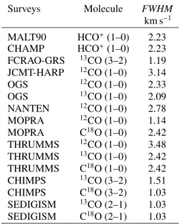
The spectrum is deconvolved from a Gaussian of fixed size adapted to each survey–molecule pair. The FWHM of this Gaus-sian is fixed a priori and is set by the median FWHM obtained on fiducial fits made for each line–survey pair (4000 spectra per pair). The values are given in TableA.1. The deconvolved sig-nal is in first approximation an inhomogeneous train of diracs. As a first approximation, its Fourier transform is a sum of com-plex exponentials whose phase is modulated by the VLSR cen-troid of each peak. Prony’s method is suitable for compressing the representation of this signal into an exponential sum. The
Table A.1. Initial FWHM values given for the spectral lines fit.
Surveys Molecule FWHM km s−1 MALT90 HCO+(1–0) 2.23 CHAMP HCO+(1–0) 2.23 FCRAO-GRS 13CO (3–2) 1.19 JCMT-HARP 12CO (1–0) 3.14 OGS 12CO (1–0) 2.33 OGS 13CO (1–0) 2.09 NANTEN 12CO (1–0) 2.78 MOPRA 12CO (1–0) 1.14 MOPRA C18O (1–0) 2.42 THRUMMS 12CO (1–0) 3.48 THRUMMS 13CO (1–0) 2.42 THRUMMS C18O (1–0) 2.42 CHIMPS 13CO (3–2) 1.51 CHIMPS C18O (3–2) 1.03 SEDIGISM 13CO (2–1) 1.03 SEDIGISM C18O (2–1) 1.03
approximation takes place here in Fourier space. The order com-pression of the model is based on a singular value decomposition of the Hankel matrix associated with the discrete Fourier trans-form of the auxiliary signal which makes it possible to separate and threshold the significant components of the exponential sum by thresholding above the noise level ≥3 or 5σ. This method is described inPotts & Tasche(2010),Peter et al.(2015),Liao &
Fannjiang(2016).
3. Multi-Gaussian fit of the spectrum.
A separable nonlinear least-squares fit is performed taking the median FWHM for each line and the VLSR obtained from the Prony method (Golub & Peyrera 2007;Osborn 1975,2007). The fit is constrained in FWHM and is based on the Trust Region Reflective algorithm (TRF,Branch et al. 1999). The algorithm runs up to give a minimum difference between the fitted and the observed sprectrum. For each source, the final output of the fit shows the original spectrum and the lines fitted with the multi-Gaussian fit process described above, together with their associ-ated VLSRpeak, as shown in Fig.2.
Appendix B: Dips detection in the H
i
profiles 0 20 40 60 80 100 120T [K]
All local extrema
minima maxima 0 20 40 60 80 100 120
T [K]
Rising & falling edges > 3.0 rms
Rising Falling 200 150 100 50 0 50 100 150
vlsr [km/s]
0 20 40 60 80 100 120T [K]
HI Self-absorption dips > 3 rms
Fig. B.1. Example of HISA identification for the source HIGALBM329.2039+0.7101 with assigned VLSR= −63.562 km s−1. The H
i
profile is plotted in black. The horizontal thick gray line shows the rms noise (σnoise) and the red dashed line shows the 3σnoise threshold. The black vertical dashed line and the gray shadow are the velocity of the source and the 3 km s−1 tolerance. The upper panel shows the identification of minima and maxima. The middle panel shows the identification of the falling and rising sides of the dip. The lower panelshows the final dips selection.In order to solve the KDA, we developed a code to analyze the dips in H
i
spectra (see Sect.3.4). The code first identifies all the extrema (Fig. B.1upper panel) and then selects only the ones above three times the noise level (σnoise). A dip is then defined as the intersection between a rising edge and a falling edge (dis-played by the arrows in Fig.B.1– middle panel) linking a min-imum to its two nearest maxima. In addition, the amplitude of the two edges must be larger than 3σnoise to be considered as significant. In this frame, the smaller and/or the overly irregular (partially refilled, asymmetric, one edge below 3σnoise) dips are not kept by the code (Fig.B.1lower panel).Appendix C: BGPS and ATLASGAL comparison
To better evaluate the reliability of our distance determination we use the comparison of ATLASGAL and BGPS catalogs as a reference. There are 697 sources with distance in common in these two samples. FigureC.1(a) shows that they have velocity in good agreement with 92% (634 sources) of them having a veloc-ity difference ≤5 km s−1. FigureC.1(b) shows the typical shape due to the differences in the distance disambiguation (as for Figures10and11sources in the ±12◦toward the Galactic center direction were discarded). We find that ∼50% (324) of sources have a distance difference ≤0.5 kpc (the typical uncertainty of the BGPS distances).
Fig. C.1. Velocity (a) and distance (b) comparison between paired BGPS and ATLASGAL sources. The red dash-dotted line is the y= x line.
Appendix D: Additional figures
Fig. D.1.Same as Fig.12(a) and (b) but without the error bars.