Operator-valued Kernel-based Vector Autoregressive Models for Network Inference
Texte intégral
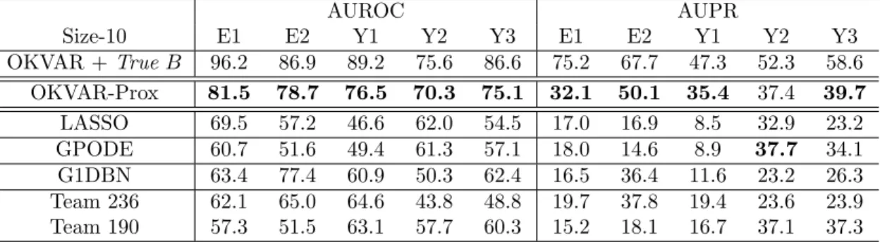
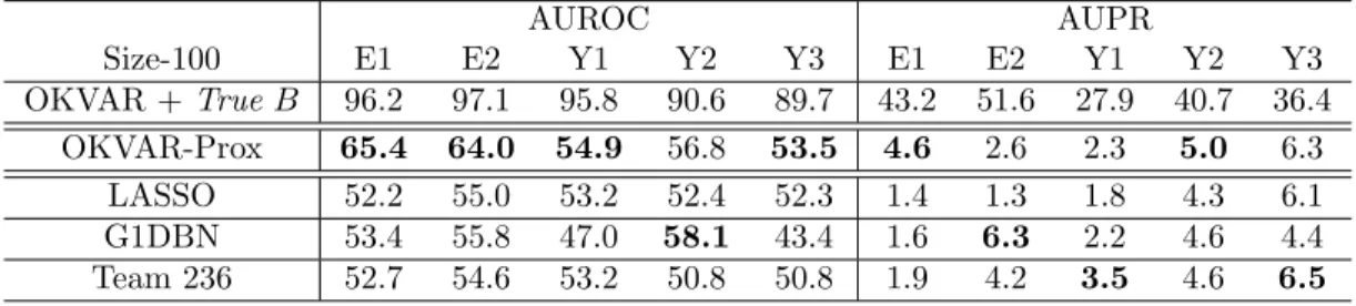
Figure


Documents relatifs
Thus, the aim for operational considerations is to estimate the error asso- ciated with the “self preservation” hypothesis, which is well suited (and up to now largely used)
† Keywords: heat kernel, quantum mechanics, vector potential, first order perturbation, semi-classical, Borel summation, asymptotic expansion, Wigner-Kirkwood expansion,
To enrich the model which can be based on Formula (1), it is possible to associate different thresholds (weak preference, preference, weak veto, veto; see, e.g., [BMR07]) with
Introduction Models Disaggregation Rank Illustration Inference Implementation On the rank of a bipolar-valued outranking
Czech mountain ski resorts – origin of visitors (authors, based on data from T-Mobile) The data from the mobile network was only one of the sources - it supplements the
This paper investigates the lag length selection problem of a Vector Error Correction Model (VECM) by using a convergent information criterion and tools based on the
It yields two different asymptotic behaviors for the large local densities and maximal value of the bifurcating autoregressive process.. Keywords: Branching process,
Then there exists a real analytic family of real analytic vector fields {XQ +/Ys} tangent to V, with an algebraically isolated singularity at 0 parametrized by a connected
