HAL Id: halshs-02652165
https://halshs.archives-ouvertes.fr/halshs-02652165
Preprint submitted on 2 Jun 2020HAL is a multi-disciplinary open access
archive for the deposit and dissemination of sci-entific research documents, whether they are pub-lished or not. The documents may come from teaching and research institutions in France or
L’archive ouverte pluridisciplinaire HAL, est destinée au dépôt et à la diffusion de documents scientifiques de niveau recherche, publiés ou non, émanant des établissements d’enseignement et de recherche français ou étrangers, des laboratoires
Optimal lockdown in altruistic economies
Stefano Bosi, Carmen Camacho, David Desmarchelier
To cite this version:
Stefano Bosi, Carmen Camacho, David Desmarchelier. Optimal lockdown in altruistic economies. 2020. �halshs-02652165�
WORKING PAPER N° 2020 – 30
Optimal lockdown in altruistic economies
Stefano Bosi
Carmen Camacho
David Desmarchelier
JEL Codes: C61, E13, I18, O41
Optimal lockdown in altruistic economies
∗
Stefano BOSI
†, Carmen CAMACHO
‡, David DESMARCHELIER
§May 22, 2020
Abstract
The recent COVID-19 crisis has revealed the urgent need to study the impact of an infectious disease on market economies and provide adequate policy recommendations. In this regard, we consider here the SIS hypoth-esis in dynamic general equilibrium models with and without capital accu-mulation, and we compute the efficient lockdown of altruistic agents. We find that the zero lockdown is efficient if agents are selfish, while a positive lockdown is recommended beyond a critical level of altruism. Moreover, the lockdown intensity increases in the degree of altruism. Our robust analytical results are illustrated by numerical simulations, which show, in particular, that the optimal lockdown never trespasses 60% and that eradication is not always optimal.
JEL codes: C61, E13, I18, O41.
Keywords: optimal lockdown, SIS model, Ramsey model.
1
Introduction
On December 31st, the Chinese WHO office was informed of cases of pneumo-nia of unknown origin in the city of Wuhan. On the 11th and 12th January, the Chinese authorities identified a new type of coronavirus as the cause of the illness. On January the 23rd, there were 571 cases and 17 deaths. Dreading the rapid expansion of the illness, the Chinese government decided on that date to lock down the city of Wuhan and the neighboring region, affecting a total of about 57 million people. Only a share of healthy individuals of a household could go out, once a day, and only for essential shopping. The economic activity fell and the world feared a recession. Within one month, the rest of the world had to face the same problem. On the 11th of March 2020, the World Health Organization (WHO) declares that epidemic had become a pandemic. The dif-ficult question all policy-makers need to face is the extent of the lockdown. Can ∗The authors would like to thank Cuong Le Van for his helpful comments and suggestions. Stefano Bosi acknowledges the financial support of the E3 Project of the University Paris-Saclay.
†EPEE, Université Paris-Saclay. E-mail: [email protected]. ‡PJSE (UMR 8545), PSE. E-mail: [email protected].
a country stop the epidemic while maintaining some economic activities? All activities? The present paper proposes a series of three nesting stylized models of lockdown, establishing the feedback between the pandemic and production.
The urgency of the epidemiological issue and its economic consequences has led a number of specialists in economic dynamics in a race against time to recommend policy solutions. Acemoglu et al. (2020), Alvarez et al. (2020), Atkeson (2020) and Eichenbaum et al. (2020) introduce a SIR epidemiological assumption in an infinite-horizon general equilibrium model without capital ac-cumulation. In the SIR model, population splits in three groups: Susceptibles (S), Infectives (I) and Removed/Recovered individuals (R). The SIR’s main assumption is that recovered individuals develop a lifelong immunity, that is, they cannot contract the disease again. In particular, in Alvarez et al. (2020) a policy-maker minimizes simultaneously the discounted value of fatalities and the output costs of the lockdown. Because of the interplay between the epi-demic dynamics and the lockdown, the problem is non-convex. The authors provide numerical simulations using the recent preliminary data on COVID-19. In all their scenarios, the optimal policy starts with a severe lockdown of at least 60%, which is gradually lessened. The disease disappears in the long run in all considered scenarios. Going further, Acemoglu et al. (2020) build a multi-risk SIR model considering three age groups who suffer differently from the COVID-19 pandemic. Even further, their model also explores the impact of social distancing, testing and the arrival of a vaccine on optimal policies. Given the complexity of the problem and its stochastic nature, the authors are obviously obliged to resort to numerical simulations as well. They show that imposing targeted lockdown measures, social distancing and increasing testing minimize economic losses and deaths. In all scenarios, whether semi-targeted or uniformly targeted policies are chosen, a positive lockdown is always adopted while waiting for the vaccine. Finally, let us mention Gollier (2020), who also an-alyzes a multi-risk SIR model with three population groups. Among the family of reasonable policies, Gollier (2020) notices the existence of two polar solutions "potentially optimal". On the one hand, a lockdown of 90% during four months will succeed eradicating the pandemic. On the other, a lockdown of 30% for five months which allows to flatten the curve. The cost of both strategies is similar, a 15% of annual GDP. In all three papers, the policy maker takes into account deaths as a cost which is equal to a life’s statistical value.
Our paper aims at exploring other directions. To date, epidemiologists seem doubtful about the degree and duration of COVID-19 immunity. Note that optimal lockdown policy is clearly sensitive to the assumption of permanent immunity. To date, there is no consensus about the duration of immunity but for a majority of virologists the period is plausibly short (see, for instance, the WHO COVID-19 daily press briefing on the 13th of April 2020). This lack of consensus presses the scientific community to open their research lines and search for robust policy recommendations under all possible scenarios for immunity. In this context, the Susceptible-Infected-Susceptible (SIS) model represents an interesting alternative to the SIR framework. The SIS approach considers indeed the opposite case and, in a way, the worst: recovery does
not confer immunity. More precisely, the population is divided in two groups: Susceptibles (S) and Infectives (I). A susceptible can contract the disease after a contact with an infective and, then, get back to the group of susceptibles after recovery.
Note that in SIS models, mortality is zero. As a result, a SIS model cannot explain the mortality and immunity of the COVID-19. However, it can pro-vide with important and relevant insights since the COVID-19 mortality rate is low compared to other diseases. Additionally, as previously mentioned, the immunity period is apparently short. Historically, the SIS model has been used to represent the spread of bacterial diseases as meningitis and plague, or the spread of protozoan diseases as malaria or the sleeping sickness (see Hethcote, 1976).
The hybrid literature combining economics and epidemiology dates back to the early Seventies. In one of the seminal contributions, Sanders (1971) minimizes the social cost of an epidemic finding the optimal treatment in a SIS model. Because of the constant marginal cost of the treatment, a bang-bang solution is obtained: either the effort of the public health system is at its maximum and the disease eradicated; or the public health system does not make any effort and the disease grows out of any control (see also Sethi, 1974). The same minimization program was reconsidered in Goldman and Lightwood (2002) although with a more general social cost function. The authors provide conditions ensuring the optimality of the disease-free steady state. Identical conclusions were reached by Gersovitz and Hammer (2004) and Barrett and Hoel (2007) with a vaccination protocol instead of a treatment effort. To the best of our knowledge, the first attempt to introduce the SIS hypothesis in an economic growth model is Goenka and Liu (2012). Like them, we also consider an infinite-horizon model, but, instead of considering a centralized economy a la Ramsey, we work with a general equilibrium model based on market mechanisms in the spirit of Bosi and Demarchelier (2018).
The main objective of the present paper is to provide policy makers with robust optimal recommendations in face of an epidemic of the SIS type. Our determination to provide exact optimal policies will force us to assume that the lockdown is constant in time. As a result, we model here a government who chooses the lockdown level that maximizes a measure of inter-temporal social welfare over an infinite time horizon. Welfare is understood here in a large sense since it embraces empathy towards infectives. In particular, welfare de-pends, as usual, on households’ consumption but also on the share of infectives which is a negative externality: the more infectives, the less the household en-joys consumption. It is important to add a few words on empathy. Empathy is one of the key features of the COVID-19 pandemic and of the present pa-per. Without empathy the extreme lockdown measures imposed all over the world could not be understood. Certainly, the virus is fatal mainly for retired individuals: a 6% of all infected over 65 years dies (see Ferguson et al., 2020). The economic loss that follows the lockdown would be way too high according the pure economic reasons. The recent literature mentioned above introduces fatalities in the policy maker’s objective as statistical economic losses. Among
them, only Acemoglu et al. (2020) consider a measure of empathy, in this case, an emotional cost of death. We also believe that empathy towards the infected plays a major role in political and economic decisions, and as a consequence, we assume that individuals maximize their overall welfare, which depends as usual on consumption, and also on the share of infectives in the society.
We construct three embedded models which correspond to two different wel-fare measures and which include, or not, the accumulation of wealth. More explicitly, we study first the optimal lockdown prescribed by the Ramsey cri-terion. In the Ramsey criterion, all generations are equally important to the policy maker. Although ethically fair, it presents a major technical challenge since overall welfare cannot be computed over an infinite period. Ramsey (1928) proposed to maximize welfare as the distance of actual welfare to a bliss point. For any level of altruism, we obtain the explicit forms for the optimal lockdown, the evolution of the epidemic and the household’s consumption. Without empa-thy, the policy maker optimally chooses a zero lockdown, while under empathy a positive lockdown is optimal. In both cases, the economy converges to the endemic steady state: in the long run it is optimal to accept a permanent num-ber of infectives in order to avoid unbearable economic and social costs even if agents are altruistic.
Next, we use the Cass-Koopmans criterion (1965) to describe the policy maker’s representation of welfare. Here, households’ utility is discounted in time so that future generations weight less in overall welfare. The Cass-Koopmans criterion is more difficult to solve, but still we are able to find the long-run solution. If we focus on maximizing long-run welfare, a positive level of lockdown remains optimal. However, the eradication of the disease is efficient only if households are empathetic towards infectives. When welfare is maximized along the transition, the optimal lockdown is positive only beyond a critical degree of altruism. Nevertheless, the optimal lockdown may be here insufficient to eradicate the epidemic, in contrast with some pure epidemiological models.
Finally, we introduce capital accumulation in the previous Cass-Koopmans model to appreciate the impact of the lockdown on the wealth of a nation. We obtain the same qualitative results as in the basic model without capital and, in this sense, our conclusions seem quite robust.
As already mentioned, we use numerical exercises to illustrate our theoretical results and optimal policy recommendations. We calibrate the models using the most updates COVID-19 data, in line with the recent literature. Among all results, let us advance that the optimal lockdown is always lower than 60%, as in Alvarez et al. (2020) and Acemoglu et al. (2020). Although our frameworks are different, a SIR model with very low mortality and a SIS model, where mortality is zero, are relatively close. Our results reveal the real weight of the epidemics in the economy since whatever the cost or welfare function, all the recent research find there is a critical value of 60% never to trespass.
The rest of the paper is organized as follows. Sections 2 presents the SIS model under consideration, and it obtains the explicit trajectory for the share of infected. Section 3 presents the economic framework. Then Sections 4 and 5 present and analyze the epidemic-augmented infinite-horizon models without
capital accumulation and the growth model. Finally, Section 6 concludes. All proofs are gathered in the Appendix.
2
Epidemiology
At time t total population is divided in infectives and susceptibles of contracting a disease. Let N (t), I (t) and S (t) denote total population, infectives and susceptibles at time t, then:
N (t) = I (t) + S (t) Let
x (t) ≡ I (t) N (t) be the share of infectives in total population.
To contain the epidemic, the government decides to impose a lockdown, which will stay constant over time. Let λ ∈ [0, 1] denote the share of locked down citizens.1 The number of infectives and susceptibles in circulation are
given by
(1 − λ) I (t) = (1 − λ) x (t) N (t) and (1 − λ) S (t) = (1 − λ) [1 − x (t)] N (t) (1) One of the key characteristics of an epidemic is the way it transmits be-tween two humans who get close enough. We assume that each individual in circulation meets a fixed number ν of people per period. In this case, an infective in circulation meets ν [1 − x (t)] susceptibles on average. The to-tal number of meetings between infectives and susceptibles in circulation is given by ν [1 − x (t)] (1 − λ) I (t) and the total number of new infectives by pν [1 − x (t)] (1 − λ) I (t), where p is the susceptible’s probability of getting sick during a meeting with an infective. The infectivity rate p is disease-specific.
Thus, the number of new infectives is given by ˙
I (t) = [µ (1 − λ) [1 − x (t)] − m − r] I (t) (2)
where µ ≡ νp. m and r are the mortality rate and the recovery rate of infectives. Population evolves according to a simple law:
˙
N (t) = nN (t) − mI (t) (3)
where n denotes the net rate of population growth without the mortality due to the infectious disease.
1Contrary to Alvarez et al. (2020) and to Acemoglu et al. (2020), the lockdown level is not constrained by an upper bound less than one. A policy-maker could in principle lock down all population if she found it optimal. Although this could indeed be the case in the pure epidemiological model, we will prove that it is never optimal to confine all the labor force.
Dividing (2) and (3) by N (t), we obtain ˙ I (t) N (t) = (µ (1 − λ) [1 − x (t)] − m − r) (1 − [1 − x (t)]) (4) ˙ N (t) N (t) = n − mx (t) (5) Observe that ˙x (t) = d dt I (t) N (t) = ˙ I (t) N (t)− I (t) N (t) ˙ N (t) N (t) = ˙ I (t) N (t)− x (t) ˙ N (t) N (t) Then, substituting ˙I (t) /N (t) and ˙N (t) /N (t) into ˙x:
˙x (t) = x (t) ([1 − x (t)] [µ (1 − λ) − m] − n − r) (6) which represents the reduced epidemiological dynamics.
Let us introduce the following critical values for the lockdown and the share of infectives, which are key references in the sequel:
λ1≡ 1 − m + n + r µ , λ2≡ 1 − m µ and x1≡ 1 − n + r µ (λ2− λ) (7) The following plausible assumption means that the number of meetings ν has to be large enough for the illness to become and epidemic and hence, subject of concern.
Assumption 1
µ > m + n + r
Note that Assumption 1 implies 0 < λ1 < λ2 < 1. Next, we solve (6) and
completely characterize x.
Proposition 1 (epidemiological dynamics) Let Assumption 1 hold. The share of susceptibles is
x (t) = x0x1
x0+ (x1− x0) eµ(λ−λ1)t
(8) with x0≡ x (0), the initial share of susceptibles.
There are two stationary states:
(i) a disease-free steady state, that is ¯x = 0;
(ii) an endemic steady state in which ¯x = x1∈ [0, 1].
The endemic steady state exists if and only if the lockdown rate λ is below the first threshold: λ ≤ λ1. When λ = λ1, the endemic and the disease free
steady state coincide.
The evolution of x in time crucially depends on the lockdown λ:
(1) if 0 ≤ λ < λ1, then x (t) increases (decreases) continuously from x0 to
x1 > 0 if x0 < x1 (x0 > x1). If λ < λ1, the steady state ¯x = x1 ∈ (0, 1) is
globally stable and the steady state ¯x = 0 globally unstable.
(2) if λ1 ≤ λ ≤ 1, then x (t) decreases continuously from x0 to ¯x = 0 and
Proof. See Appendix A.
Proposition 1 shows that a policy locking down a share of the population is effective in the control of epidemics, with complete eradication it if the lockdown is strong enough. Indeed, when the lockdown is strong (λ ≥ λ1), the system
converges asymptotically to a solution with no disease. On the contrary, when the lockdown is light (λ < λ1), the system converges to the endemic steady
state with a strictly positive number of infectives.
There exists one important index in the epidemiological literature: R0. R0is
the basic reproduction number of a disease representing its transmissibility. In our model, we can compute R0as a function of the fundamental parameters and,
then, understand its determinants. In particular, we can show that R0 drives
the convergence to the endemic steady state and that it can be reinterpreted in terms of the critical lockdown λ1. Let us see how. In the spirit of Hethcote
(2000), we introduce the average number of new infectives generated by one infective as
R (λ) ≡ µ
n + r(λ2− λ)
Observe that according to (7) and under the plausible assumption that λ < λ2,
x1> 0 ⇔ R (λ) > 1
that is, the economy converges to an endemic steady state with a positive share of infectives if and only if R (λ) > 1.
Moreover, the critical value R (λ) can be reinterpreted in terms of a critical lockdown. Indeed, since
R (λ) = 1 + µ
n + r(λ1− λ) we find that
R (λ) > 1 ⇔ λ < λ1
where λ1is the bifurcation point of the dynamics of x, given in (8).
Here we define R0as
R0≡ R (0) =
µ − m
n + r (9)
In order to understand why R0represents the basic reproduction number in
a naïve population (where basic means λ = 0 and naïve x = 0), let us focus on a simplified model with m = n = 0. In this case, according to (7),
R0= µ
r (10)
Consider now a group of quarantined infectives. Because of the recovery rate, the number of infectives declines over time: I (t) = I (0) e−rt
. The average duration of illness in this group is given by
D =
∞
0
re−rt
and the average number of new infectives generated by an infective in a naïve population by pν (1 − x) = pν = µ times the average duration D, that is by R0= µ/r.
To conclude this section, let us numerically illustrate the dynamics of x. Our exercises aim at highlighting the role of the lockdown on the dynamics of x, and its convergence towards an endemic or a disease-free steady state. All the paper’s calibration details can be found in Appendix H. Let us just add here a few words on R0 and r. Only to mention two recent articles, Acemoglu et al. (2020) use
a value of R0= 3.6 to align with Alvarez et al. (2020). However, Acemoglu et
al. (2020) consider the value too high and perform some of their exercises using R0 = 2.4, as in Ferguson et al. (2020). In Gollier (2020), R0 depends on the
group age. It ranges from 2.84 for the young, 2.64 for the medium age and 1.08 for seniors. Gollier (2020) also computes an ex-post overall R0 of 2.37, after all
the basic prevention measures were taken in France. Here, R0= 2.49 following
recent estimations done by the research group MIVEGEC/ETE at Montpellier University. Hence, our choice for R0is at the same time, aligned with the most
updated estimations for France and with the recent literature on the COVID-19 pandemic. Regarding the illness duration, 1/r, Alvarez et al. (2020) and Acemoglu et al. (2020) consider 18 days, whereas in our benchmark is slightly lower, 14 days. In Gollier (2020), people recovers after 2 or 3 weeks on average.
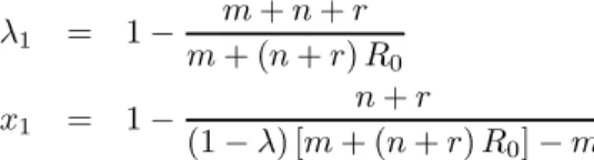
We observe that, using (7) and (9),
λ1 = 1 −
m + n + r m + (n + r) R0
x1 = 1 − n + r
(1 − λ) [m + (n + r) R0] − m
Figure 1 shows two scenarios for the evolution of infectives. On the left panel, the lockdown rate is λ = 1/3 < λ1 = 59.83% and x converges towards
the endemic steady state. There will always be a 39.76% of infectives in the long run.
On the right panel, the lockdown is above the critical value: λ = 2/3 > λ1=
59.83%, and the disease is rapidly eradicated (indeed, in this case x1< 0).
Endemic steady state Disease-free steady state
These are hypothetical and possible trajectories where λ is chosen arbitrar-ily. Next, let us introduce the economic assumptions of the model to provide foundations for the choice of λ.
3
Economics
As seen in the introduction, the hybrid theoretical literature on the economic consequences of infectious diseases and the relevant policy recommendations is flourishing. The literature on infinite-horizon economies, pioneered by Goenka and Liu (2012) and developed recently by Acemoglu et al. (2020), Alvarez et al. (2020), Atkeson (2020), Eichenbaum et al. (2020), Gollier (2020), or Piguillem and Shi (2020), mainly focuses on the optimal lockdown under a permanent immunity (the so-called SIR hypothesis) within a centralized Ramsey model. In contrast, we consider here a SIS mechanism at work in a decentralized market economy. Recall that under the SIS assumption, individuals do not get immunity after recovery and can get infected again.
For simplicity, let us fix m = n = 0 in equation (3) so that population becomes constant over time ( ˙N (t) = 0). The critical points λ1 and x1 in(7)
become λ1≡ 1 − r µ, λ2≡ 1 and x1(λ) ≡ 1 − r µ (1 − λ) (12)
All the susceptibles in circulation work and only them. For the sake of simplicity, teleworking is not allowed. The labor force is then given by: L (t) ≡ (1 − λ) [1 − x (t)].
As explained in the Introduction, people care about infectives. To capture this, we let individuals’ utility depend on a composite good
G (t) ≡ ˜G (c (t) , 1 − x (t))
which is a function of individual consumption, c (t), and the share 1 − x (t) of susceptibles. Note that since agents can not chose the share of infectives, the empathy for the suffering of others is a negative externality for the household.
Assumption 2 ˜G is increasing in c (t) and 1 − x (t), and homogenous of degree one.
Here for instance we consider the following Cobb-Douglas specification in all examples:
G (t) ≡ c (t)1−α[1 − x (t)]α (13)
with 0 ≤ α < 1. Here α captures the degree of altruism. When α = 0, the agent is selfish; when α > 0, she is altruistic.
For simplicity, all households are identical. Since households live forever and population is constant over time, welfare maximization is equivalent to utility maximization.
The government maximizes the following utility functional with respect to the lockdown degree:
W (λ) ≡
∞
0
e−ηθt
with η = 0, 1. θ is the time discount rate, u = u (G) represents instantaneous utility and ¯G is defined as
¯
G = ˜G (¯c, 1 − ¯x)
is the stable (either endemic or disease-free) steady state. u( ¯G) is the bliss point considered by Ramsey (1928) and mentioned in the Introduction. As it is usual, we establish the following assumption regarding the utility function.
Assumption 3 The felicity function u is increasing ( u′
(G) > 0) and con-cave ( u′′
(G) ≤ 0).
The elasticity of intertemporal substitution is given by ε (G) = − u
′(G)
Gu′′(G) (15)
A standard functional form often considered to measure utility is u (G) ≡ CG 1−1 ε 1 −1 ε (16) with C > 0, which has the appealing property of a a constant elasticity: ε (G) = ε > 0. Note that since the arg maxλ∈[0,1]W (λ) does not depend on C when the
utility functional is separable, we normalize C to one.
Recall that the purpose of our model is to compute the optimal lockdown λ∗
, that is the level of λ which maximizes the welfare criterion W in (14): λ∗
≡ arg max
λ∈[0,1]W (λ)
In the following, we consider two different criteria of welfare maximization depending on η:
(1) the Ramsey criterion with η = 0. Here, agents do not discount future and the bliss point u ¯G is taken into account.
(2) the Cass-Koopmans criterion with η = 1. Contrary to case (1), agents discount the future without referring to a bliss point: the welfare functional boils down to the standard utility functional (Cass, 1965; Koopmans, 1965).
Regarding the economic assumptions, we consider first a basic model without capital accumulation in Section 4, and then a model with capital accumulation (growth model) in Section 5.
4
A basic model
In this economy the labor force is the only input and, for simplicity, the pro-duction function is linear:
F (L (t)) = AL (t)
Output is entirely consumed, so that denoting by c (t) individual consump-tion, we have that N (t) c (t) = F (L (t)). Therefore, individual consumption is given by
Notice that this amount of consumption is equivalent to the market solution with a full pandemic insurance. Indeed, profit maximization yields: w (t) = A, where w (t) is the unit wage at time t. A full worker’s insurance implies that N (t) c (t) = wt(1 − λ) St= A (1 − λ) [1 − x (t)] N (t) and, finally, (17).
Under Assumption 2, the composite goods becomes G (t) = g (A (1 − λ)) [1 − x (t)] where
g (A (1 − λ)) ≡ ˜G (A (1 − λ) , 1)
Let us assume that g (0) = 0 and let us define the elasticity of the composite good as
A (1 − λ) g′
(A (1 − λ))
g (A (1 − λ)) ∈ (0, 1)
and the degree of altruism (empathy) as: α (A (1 − λ)) ≡ 1 −A (1 − λ) g
′
(A (1 − λ)) g (A (1 − λ))
In the sequel, we consider a constant degree of altruism: α (A (1 − λ)) = α and, more explicitly, the Cobb-Douglas composite good defined in (13). Notice that, when α = 0 (selfishness), agents do not care about the infectives and the composite good equals consumption: G (t) = c (t).
4.1
The Ramsey criterion
This first subsection computes the optimal lockdown rate when the policy maker uses the Ramsey criterion to measure welfare, this is, η = 0 in (14). We adopt here the simplest felicity function, i.e. the identity:
u (c) = c (18)
corresponding to a felicity function with an infinite elasticity of intertemporal substitution, that is, ε = ∞.
In this case, we can compute the optimal lockdown degree, that is the value of λ which maximizes the welfare functional:
W (λ) ≡ ∞ 0 G (c (t) , 1 − x (t)) − ¯G dt = g (A (1 − λ)) ∞ 0 [¯x − x (t)] dt (19) Proposition 2 (optimal lockdown) Let Assumptions 1, 2 and 3 hold and the degree of altruism be constant. Then
(1) If agents are selfish (α = 0) and x0< 1 − r/µ, then the optimal solution
is zero lockdown: λ∗
(0) = 0. In this case, the economy converges to the endemic state limt→∞x (t) ≡ x1= λ1> 0 along the trajectory
x (t) = x0λ1
(2) If agents are altruists (α > 0); then for any lockdown degree λ∗
∈ (0, λ1),
there always exists a degree of altruism α ∈ (0, 1) such that λ∗
is optimal: λ∗
= arg maxλ∈[0,1]W (λ) ∈ (0, λ1). In this case, the economy converges to the
endemic state limt→∞x (t) ≡ x1(λ∗) > 0 along the trajectory
x (t) = x0x1(λ ∗ ) x0+ [x1(λ ∗ ) − x0] eµ(λ ∗−λ 1)t
Furthermore the optimal lockdown degree increases in the degree of altruism: λ∗′
(α) > 0.
Proof. See Appendix B.
Using (17) one can understand the opposite effects that the lockdown has on labor supply and consumption. On the one hand, when λ increases more workers are locked down, labour supply lowers and, as a consequence, both the levels of production and consumption decrease. On the other hand, the num-ber of infectives lowers as λ increases, augmenting labour supply jointly with production and consumption. When agents are selfish (α = 0), the negative effect always dominates the positive one. Indeed, without altruism welfare de-pends only on consumption, and, as a result, the consumption loss from a more severe lockdown has a negative effect on welfare. Therefore, a zero lockdown is always recommended to minimize this loss. Conversely, when agents are al-truistic (α > 0), a substitution mechanism takes place: households are willing to accept a lower consumption in exchange for more healthy people. Here, the optimal policy is a positive lockdown. In both cases, because of the economic effects of the lockdown, it is efficient to reach an endemic steady state with a positive share of infectives. This is in marked contrast with the recommenda-tions of most epidemiologists very intended to eradicate the disease as quickly as possible (see Ogura and Preciado, 2017, among others). As expected, even the simplest model encompassing epidemics and economics finds there is a conflict between health and production, which only empathy can overcome.
To complete this subsection, let us illustrate our results numerically. Figure 2 shows the optimal lockdown rate, λ∗
, as a function of altruism, α, and the optimal welfare level when λ = λ∗
, also as a function of α. As Proposition 2 proves, λ∗
increases with α. Note that λ∗
is positive only when altruism is powerful enough. Under the exercise assumptions, government facing selfish agents does not confine the population. Note that optimal welfare W (λ∗
) also increases with altruism. Hence, despite the increasing level of lockdown and the associated decrease in consumption, individuals enjoy better and feel more than compensated because of the lower share of infectives. Finally, and noteworthy, the lockdown level is always smaller than λ1. As a consequence, the number
will be a share of infectives forever.
Fig. 2 Ramsey criterion
4.2
Cass-Koopmans criterion
We focus next on the Cass-Koopmans welfare criterion, that is, the case η = 1 in (14): W (λ) ≡ ∞ 0 e−θt u (G (t)) dt (20)
The government can adopt either a naive or a sophisticated strategy, that is, respectively,
(1) a welfare maximization at the steady state to find the optimal lockdown λS in the long run.
(2) an intertemporal welfare maximization along the transition to find the optimal lockdown λ∗
from t = 0.
Let us focus first on the naive strategy. Here, the policy-maker maximizes ¯
W (λ) ≡
∞
0
e−θtu ¯G (λ) dt (21)
Proposition 3 (optimal lockdown in the long run) Let Assumptions 1, 2 and 3 hold, and let us maximize the criterion of welfare evaluated at the steady state (21). Then,
(1) If agents are selfish (α (A (1 − λ)) = 0), the optimal lockdown is an interval of values: {λS} = [0, λ1].
In this case, if 0 ≤ λS < λ1, the economy converges to x∗ = x1 > 0; if on
the contrary λS = λ1, then the economy converges to ¯x = x1= 0.
(2) If agents are altruistic, (α (A (1 − λ)) > 0), then the optimal lockdown is λS = λ1= 1 − r/µ.
In this case, the economy converges to ¯x = 0.
Proof. See Appendix C.
Surprisingly, when agents are selfish, the optimal lockdown is a continuum of values, meaning that the policy-maker is indifferent between an infinite number
of lockdown degrees. Let us analyze why. When α = 0, welfare (utility) depends only on consumption. As previously seen, the lockdown has opposite effects on production and consumption. It has first a negative impact on production because of the lower share of agents at work and, second, a positive impact because of a lower share of infectives, who are unable to work. Interestingly, at the endemic steady state ¯x = x1, the decrease in 1 − λ compensates exactly the
increase in 1 − x, as in the Ramsey criterion. As a result, according to (12) and (17), long-run consumption is given by:
cE= A (1 − λ) (1 − x1) = Ar
µ (22)
which is independent of λ ∈ [0, λ1]. Hence, the government is indifferent to the
level of lockdown in this interval.
When agents are altruistic, i.e. α > 0, utility depends not only on consump-tion but also on the share of infectives. If λ < λ1, the opposite long-run effects
of the lockdown on consumption cancel each other as before and as shown in (22). If λ > λ1, then the lockdown is strong enough and the disease disappears
in the long run. Welfare at the steady state does no longer depend on the share of infectives but only on consumption, which is now decreasing in λ since: cF = A (1 − λ). Thus, the lockdown level λ = λ1 maximizes both consumption
and social welfare in the interval [λ1, 1]. Summing up, welfare increases in λ
when λ < λ1, and decreases when λ > λ1, reaching its maximum at λ = λ1.
Next, let us introduce two critical altruism degrees, which are important thresholds for altruism:
αλ ≡ 1 − x0 x2 1 µθx1(x1− x0) (1 − λ)2+ rx0(λ − λ1) [µ (λ − λ1) − θ] (1 − x0) (1 − λ) [µ (λ − λ1) − θ]2 < 1(23) α0 ≡ 1 − x0 x1 µθ (x1− x0) + rx0(θ + µλ1) (1 − x0) (θ + µλ1)2 (24) where x1 = x1(λ) according to (12). Notice that, when λ = 0, α0 = αλ.
Moreover, if 0 ≤ λ < λ1 and x0< x1, then both α0 and αλremain below 1.
The most sophisticated policy-maker’s problem in (19) is hard to solve an-alytically. Nevertheless, policy-makers do need a sufficiently robust analytical solution in order to choose the optimal level of lockdown, and understand the role of each economic and epidemic factor. Proposition 4 below provides with simple recommendations about the minimum lockdown to implement to avoid a welfare loss.
Proposition 4 Let Assumptions 1, 2 and 3 hold and let us for simplicity focus on the logarithmic felicity (ε = 1). Consider the optimal lockdown λ∗
maximiz-ing the welfare criterion 20.
(1) If α ≥ α0, then the optimal lockdown is positive: λ ∗
> 0. (2) If α ≥ αλ for any λ ∈ [0, λ1), then the optimal lockdown λ
∗
≥ λ1.
Proposition 4 reveals the existence of a threshold value for altruism, α0,
beyond which a lockdown is established. Given its importance, we need to understand how the characteristics of the epidemics will push policy-makers to confine part of the population. In order to simplify our conclusions, let us assume that
µ > |r − θ| (25)
Under Assumption 1, µ > r − θ and, hence, (25) becomes µ > θ − r. Under (25), as an intermediate step, we can compute the following derivatives:
µ 1 − α0 ∂ (1 − α0) ∂µ = 1 − 2µ µ + θ − r < 0 r 1 − α0 ∂ (1 − α0) ∂r = rx0 rx0+ θ (1 − x0) + 2r µ + θ − r > 0
With this in hand, it is straightforward to compute the partial derivatives of the threshold α0with respect to the transmissivity and recovery rates:
∂α0
∂µ > 0 and ∂α0
∂r < 0
The threshold increases with transmissibility and it decreases with the re-covery rate. The effects of µ and r are clear. However, it is R0 which draws the
attention of media, public opinion and public authorities. Hence, let us provide some recommendations in terms of R0.
While an increase in µ and a decrease in r always entail a rise in R0= µ/r,
an increase in R0 does not necessarily imply a rise in µ or a drop in r. To avoid
any ambiguity, focus only on a rise in R0 due to a simultaneous increase in µ
and a decrease in r. In this case, and with some notational abuse, we have that ∂α0
∂R0
> 0
This means that a higher transmissibility requires a higher degree of altruism in order to impose a positive optimal lockdown. Thus, paradoxically, a higher transmissibility makes the zero lockdown more likely as efficient policy. Indeed, when the transmissibility of the infectious disease increases, the government faces significant production and consumption losses if a higher share of the population is locked down to contain the disease. Hardening the lockdown is welfare-improving only if households become more altruistic and care more about infectives.
We turn now to the numerical simulation of this augmented Cass-Koopmans model. As many authors before us have put forward, to this date there is much uncertainty about the key parameters of the current COVID-19 pandemic. Obviously, the optimal lockdown policy is sensitive to the calibration and our results should be taken as illustrative. The benchmark case is given by the quarterly values of three classes of parameters referring to (1) disease: m = n = 0, r = 6, R0 = 2.49; (2) production: A = 1; and (3) preferences: α = 1/2,
We vary the main parameters α and r with respect to the benchmark to capture the impact of altruism and transmissibility on health and consumption when the policy-maker implements the optimal lockdown.
Altruism. In the first column of figure 3 below, we compare a selfish econ-omy (α = 0) with the benchmark (α = 1/2). In the first scenario, the lockdown is 0 and the economy experiences a higher endemic steady state. Meanwhile, in the case of an altruistic economy, the endemic steady state is lower because of the hard lockdown (λ∗
= 59.4%). However, this severe lockdown does not eradicate the disease. The impact on consumption is the opposite. In a selfish society, consumption falls from the initial value 0.999 to the asymptotic value 0.4016. At the beginning, selfish agents consume more because of the zero lock-down and the higher production. However, after a short lapse of time, the larger number of infectives reduces the labor force significantly, lowering consumption below the level of the altruistic society.
Transmissibility. In the second column of figure 3, we explore the role of the disease recovery rate r, keeping constant the basic reproduction number R0. Note first that varying r is equivalent to varying the disease duration 1/r.
Then observe that µ = rR0 changes with r. We compare the effects of a longer
duration (one month on average, that is r = 3) with those of the benchmark (two weeks, that is r = 6). In the first case, the transmissibility is higher than in the benchmark and the economy converges to an endemic steady state with a larger share of infectives. As above, the effects on consumption are the opposite: the lighter lockdown (58.9% < 59.4%) in the case of a longer duration (r = 3) entails a larger consumption at the beginning. When the number of infectives becomes burdensome, the economy experiences lower production and consumption than in the benchmark (r = 6). Here again, the economy converges
towards an endemic steady state in both scenarios.
Fig. 3 Cass-Koopmans criterion
5
Growth model
The classical growth model is the model by Ramsey (1928), revisited later by Cass (1965) and Koopmans (1965) with positive discounting, θ > 0. We re-consider the epidemiological dynamics (8) within this infinite-horizon economic framework.
There are many firms with a common Constant Returns to Scale (CRS) tech-nology: Yj(t) = F (Kj(t) , Lj(t)), where Kj(t) and Lj(t) are firm j’s demand
for capital and labor. Let ρ and w denote the price of capital and labor, i.e. the interest rate and wage respectively. The firm’s profit maximization problem entails that at equilibrium:
ρ (t) = f′ ˜ kj(t) (26) w (t) = f ˜kj(t) − ˜kj(t) f′ ˜kj(t) where ˜kj is defined as ˜ kj(t) ≡ Kj(t) Lj(t) and f ˜kj(t) ≡ F ˜kj(t) , 1
are the capital intensity and the (average) productivity per worker. Notice that (26) implies a common capital intensity ˜kj(t) = ˜k (t) for any firm j.
We introduce the capital share in total income:
ϕ ˜k ≡
˜ kf′ ˜
k
f ˜k (27)
Observe that positive prices (ρ (t) , w (t) > 0) require that
0 < ϕ ˜k < 1 (28)
As in the previous section, only the susceptibles in circulation work: infec-tives and confined susceptibles do not work (telework is not allowed here either). Therefore, the aggregate labor force is given by
j
Lj(t) = (1 − λ) S (t) (29)
Aggregate wealth is equal to aggregate capital and hence N (t) k (t) = j Kj(t) = j Lj(t) Kj(t) Lj(t) = ˜k (t) j Lj(t) = ˜k (t) (1 − λ) S (t)
that is k (t) = ˜k (t) (1 − λ) S (t) /N (t) or, equivalently, ˜
k (t) = k (t)
(1 − λ) [1 − x (t)] (30)
Equation (30) is the link between capital intensity and individual wealth. A key assumption here is that workers are fully insured. Whether fully em-ployed or not, they receive the same labor income ω (t). Each worker (suscepti-ble in circulation) supplies one unit of labor. Then according to (29), aggregate labor income is given by
ω (t) N (t) = w (t)
j
Lj(t) = w (t) (1 − λ) S (t)
and the value of labor income obtains as a function of the unit wage and the share of susceptibles allowed to work
ω (t) = w (t) (1 − λ) [1 − x (t)] (31)
In the Ramsey model, production is equal to consumption plus savings, which yields the following savings mechanism:
where k (t) is the individual’s wealth; ω (t) her labor income; c (t) instantaneous consumption and δ the constant depreciation rate of capital.
We consider a two-stage optimization program in which both households and the government take optimal decisions in light of the evolution of the epi-demics. First, given the lockdown degree λ announced by the public authority, the household maximizes the utility functional
W (λ) ≡ max c ∞ 0 e−θt u (G (t)) dt (33)
subject to the accumulation law for individual wealth given in (32) and where G (t) = ˜G (c (t) , 1 − x (t)). Second, the government fixes the optimal lockdown degree taking into account the consumer’s solution to program (33).
For simplicity, let us adopt a Cobb-Douglas description of the composite good with a constant degree of altruism α as defined in (13), that is, G (t) ≡ c (t)1−α[1 − x (t)]α.
Let us start with the household problem. Proposition 5 provides the dynamic general equilibrium with epidemics
Proposition 5 (general equilibrium with epidemics) Under Assumptions 1, 2 and 3, and a Cobb-Douglas composite good with degree of altruism α, the economic and epidemiological equilibrium dynamics are driven by the following dynamic system: ˙x (t) x (t) = µ (1 − λ) [x1(λ) − x (t)] (34) ˙k (t) = (1 − λ) [1 − x (t)] f k (t) (1 − λ) [1 − x (t)] − δk (t) − c (t) ˙c (t) c (t) = f ′ k (t) (1 − λ) [1 − x (t)] − δ − θ ε (G (t)) 1 − α + αε (G (t)) (35) +µ (1 − λ) x (t)x1(λ) − x (t) 1 − x (t) α − αε (G (t)) 1 − α + αε (G (t)) (36)
where the initial levels x (0) and k (0) are given, and the terminal value of con-sumption satisfies the transversality condition
lim t→∞e −θt u′ (G (t)) k (t)∂ ˜G ∂c = 0 x1(λ) is defined in (12) and G (t) is given by (13).
Proof. See Appendix E.
There are two cases in which the Euler equation (35) has a simple expression. For instance, if the utility function is logarithmic, i.e. ε (G (t)) = 1 then (36) becomes
˙c (t) c (t) = f
′ k (t)
The second case arises when agents are selfish and α = 0. Here the Euler equation (36) boils down to
˙c (t)
c (t) = ε (G (t)) f
′ k (t)
(1 − λ) [1 − x (t)] − δ − θ Notice also that (34) is equivalent to
x (t) = x0x¯
x0+ (¯x − x0) eµ(λ−λ1)t
The economy inherits two steady states from the epidemiological dynamics in (6) as explained in the following proposition.
Proposition 6 (steady states) The dynamic system (34)-(36) has two steady states, an endemic steady state with a positive number of infectives and a disease-free steady state. The endemic steady state exists if and only if 0 ≤ λ ≤ λ1.
(i) If 0 ≤ λ < λ1, then x (t) increases (decreases) continuously from x0 to
x1> 0 if x0< x1 (x0> x1). The endemic steady state (kE, cE) is given by
f′ µ rkE = δ + θ (37) cE = δ + θ ϕ µrkE − δ kE (38) where ϕ is given by (27).
(ii) If λ1≤ λ ≤ 1, then x (t) decreases from x0 to ¯x = 0 and the disease-free
state (kF, cF) is given by f′ kF 1 − λ = δ + θ (39) cF = δ + θ ϕ kF 1−λ − δ kF (40)
When λ = λ1, the endemic and the disease-free steady states coincide (x1= 0).
Proof. See Appendix F.
In case (i), the steady state (kE, cE) is independent of λ in the interval
[0, λ1). However, since ¯x = x1, then G depends on λ. Let us explain why. As
seen above, a variation in λ affects both capital and consumption. There is a first positive effect, because of the higher share of healthy workers. The second effect is negative because of the lower labor supply induced by the stronger lockdown. According to (12), the stock of capital in the long run does no longer depend on the lockdown:
f′ kE
(1 − λ) (1 − x1)
= f′ µ
In other terms, the positive effect of the lockdown on (1 − x1) exactly
com-pensates the negative effect on (1 − λ). The same happens for the stationary consumption: cE = (1 − λ) (1 − x1) f kE (1 − λ) (1 − x1) − δkE = r µf µ rkE − δkE Summing up, the lockdown has no effect on the endemic steady state in terms of capital and consumption.
In case (ii) of Proposition 6, differentiating (39) with respect to λ, we find λ kF ∂kF ∂λ = − λ 1 − λ< 0 (41)
while differentiating (40) and using (41), we obtain that λ cF dcF dλ = − λ 1 − λ < 0 (42)
Now the lockdown affects the disease-free steady state in terms of capital and consumption. Indeed, since λ has no effect on the share of infectives because the disease has been eradicated, the only effect at work is negative: the stronger the lockdown, the lower the share of workers in circulation and the labor supply, and, finally, the lower the levels of production and consumption, and the capital stock.
Example. In the case of a Cobb-Douglas production function F (Kj, Lj) =
Kjϕ, L1−ϕj , we obtain f ˜k = A˜kϕand the steady states become the following.
(i) Endemic: kE= r µ δ + θ Aϕ 1 ϕ−1 = 1 R0 Aϕ δ + θ 1 1−ϕ and cE= δ + θ ϕ − δ kE (ii) Disease-free: kF = (1 − λ) Aϕ δ + θ 1 1−ϕ and cF = δ + θ ϕ − δ kF
Next, let us solve the second stage of our strategy considering the govern-ment’s program, i.e. maxλ∈[0,1]W (λ). As with the Cass-Koopmans criterion
in section 4.2, we examine two different lines of action. In the first, the policy maker adopts a naive approach and maximizes welfare at the steady state to find the optimal lockdown in the long run, λS. In the second, welfare is maximized
along the transition to find the optimal lockdown λ∗
. Given the complexity of this second problem, we cannot provide with analytical results and we shall resort to numerical exercises to highlight the properties of the optimal lockdown.
In the naive approach, the welfare functional is evaluated at the steady state and it is given by ¯ W (λ) ≡ ∞ 0 e−θt u ¯G (λ) dt = u ¯G (λ) θ (43)
Proposition 7 (optimal lockdown in the long run) Let Assumptions 1, 2 and 3 hold. We maximize the criterion of welfare evaluated at the steady state (43) and obtain the optimal lockdown level λS:
(1) If agents are selfish, α = 0, then the optimal lockdown is an interval of values: {λS} = [0, λ1]. In this case, if 0 ≤ λS < λ1, the economy converges to
an endemic steady state ¯x = x1> 0; if λS = λ1, the economy converges to the
disease free steady state ¯x = x1= 0.
(2) If agents are altruists, α > 0, the optimal lockdown is λS= λ1.
In this case, the economy converges to ¯x = 0.
Proof. See Appendix G.
Of course, solution (51) is no longer necessarily optimal if the transition G (t) is taken into account instead of the steady state ¯G to compute the utility functional (33).
Note that, when Propositions 3 and 7 are compared, we find the same results. The introduction of capital accumulation does not change the picture and the same policy recommendations hold.
To illustrate the impact of the optimal lockdown λ∗
on growth, we provide a numerical analysis taking into account the welfare maximization along the equilibrium transition.
Our exercises aim at underlining two issues. First, the pure effect of the epidemics on economic decisions. Here, we will only explore the effect of the du-ration of the epidemics on the optimal lockdown and its economic consequences. Here, as explained in the previous sections and in Appendix H, our calibration describes the 2020 COVID19 epidemics, using the best available quarterly data. As a result, we do not let vary R0, just the less certain parameter, r. Since our
modeling is quite general, we could also explore other directions in which the epidemics affect economic decisions. Second, our results emphasize the impor-tant role of preferences and its impact on both health and production. More precisely, as in the Cass-Koopmans examples, we study the role of altruism.
Let us present the benchmark and compare different scenarios varying α (altruism) and r (transmissibility). The first column of figure 4 describes the impact of α, and the second, the effects of r.
The benchmark is given by the quarterly values of three classes of parameters referring to (1) disease: m = n = 0, r = 6, R0 = 2.49; (2) production: A = 1,
δ = 0.012741, ϕ = 1/3, k0= 1; and (3) preferences: α = 1/2, ε = 1, θ = 0.01.
Altruism. Let us compare the selfish economy (α = 0) with the benchmark (α = 1/2). When α = 0, the optimal lockdown is 0 and the share of infectives converges to x1 = 59.8%. In the altruistic economy, the steady state remains
endemic even if the lockdown is stronger (59.4%). In particular, since λ∗
the disease is not eradicated and the number of infectives converges towards x1= 1.08%. In the long run, the labor force will be reduced to a 40%. In both
scenarios, k0> kE = 22.537, which induces capital and consumption to decrease
in the long run towards the steady state. Observe that initial consumption in the selfish economy is much higher. Indeed, before the sudden rise of infectives, agents enjoy the zero lockdown by producing and consuming more. Then, the dramatic rise in the share of infectives reduces significantly the labor force and, as a result, capital and consumption fall below the altruistic benchmark levels. Transmissibility. In the second column of figure 4, we consider the impact of r. As in Cass-Koopmans exercise, R0is kept constant so that µ = rR0varies
with r. When transmissibility is higher because of the longer duration of illness (r = 3), the share of infectives is larger in the short and long run. Dynam-ics are qualitatively similar to those of the Cass-Koopmans criterion (second column of figure 3). Nevertheless, there are important differences emanating from time discounting. The future matters less and consumption decreases in the case of a longer duration (r = 3) and in the benchmark (r = 6). In both cases, the decrease in capital from k0 to kE= 22. 537 is also coherent with the
decline in consumption towards the endemic value (cE = 1. 250 4) because of
the slowdown in production. The lower lockdown in the case of longer duration (58.9% < 59.4%) also explains why capital and consumption are higher than in
the benchmark (r = 6).
Fig. 4 Growth model
6
Conclusion
Most of the recent literature considering economies under the threat of an epi-demic have introduced a SIR epidemiological hypothesis in dynamic general equilibrium models. We have made instead a SIS assumption in an infinite-horizon market economy with and without capital accumulation. The SIS ap-proach makes sense for the recent COVID-19 pandemics as long as mortality remains relatively low, and the disease does not confer complete nor durable immunity.
Additionally, this paper considers altruistic agents concerned by the share of infectives in total population and studies the impact of altruism on equilibrium trajectories. In the model without capital accumulation, the government max-imizes the social welfare by fixing once and for all the degree of the lockdown. We have computed the optimal lockdown in the case of utilitarian targets us-ing: (1) a Ramsey criterion and (2) a Cass-Koopmans criterion. If agents are selfish, the zero lockdown is efficient, while a positive lockdown is recommended beyond a critical degree of altruism. Moreover, the lockdown intensity increases in the degree of altruism. We provide also the optimal evolution of the economy to the disease-free or to the endemic steady state in the case of positive or nil lockdown.
In the model with capital accumulation, we have found similar results in analytical and numerical terms, confirming the robustness of our conclusions. Noteworthy, we find an upper bound for the lockdown not to trespass. According to our simulations, this threshold for λ∗
is λ1≈ 60% implying that locking down
more than 60% of the labor force forever is sub-optimal.
Appendices
A
Proof of Proposition 1
The solution to (6) is (8) with ˙x (t) = (1 − λ) (¯x − x0)
µx0x¯2eµ(λ−λ1)t
x0+ (¯x − x0) eµ(λ−λ1)t 2
> 0
⇔ (1 − λ) (¯x − x0) > 0 (44)
According to (6), there are two stationary states: ¯x = 0 and ¯x = x1. Since
x (t) ∈ [0, 1], an endemic steady state ¯x = x1≥ 0 exists if and only if λ ≤ λ1.
When λ = λ1, the endemic and the disease free steady state coincide (¯x = 0).
According to (8) and (44), we have the following dynamics. If x0= 0, the
economy is disease-free forever. If x0> 0, we have five cases.
(i) If 0 ≤ λ < λ1, then the endemic steady state exists: 0 < x1 < 1.
According to (44), ˙x (t) > 0 if and only if x0 < x1. if x0< x1 (x0> x1), then
x (t) increases (decreases) continuously from x0 to x1.
(ii) If λ = λ1, then, according to (6), we have ˙x (t) = − (n + r) x (t)2. Then,
x (t) decreases continuously from x0 to ¯x = x1= 0.
(iii) If λ1 < λ < λ2, then x1 < 0 < x0 and x (t) < 1. Therefore, x (t)
decreases continuously from x0 to ¯x = 0.
(iv) If λ = λ2, then ˙x (t) = − (n + r) x (t), with solution x (t) = x0e−(n+r)t.
Thus, x (t) decreases continuously from x0 to ¯x = 0.
(v) If λ2< λ ≤ 1, then x (t) < 1 < x1. Therefore, x (t) decreases
Cases (i) corresponds to case (1) in Proposition 1. Cases (ii), (iii), (iv) and (v) generate the same qualitative dynamics: if λ ∈ {λ2} ∪ (λ1, λ2) ∪ {λ2} ∪
(λ2, 1] = [λ1, 1], then x (t) decreases continuously from x0 to x∗= 0 (case (2)).
B
Proof of Proposition 2
According to Proposition (1), we compute and maximize the welfare functional (19) in four cases: (i) 0 ≤ λ < λ1, (ii) λ = λ1, (iii) λ1< λ < 1, (iv) λ = 1.
(i) If 0 ≤ λ < λ1, then the economy converges to the endemic steady state
¯
x = x1∈ (0, 1). Replacing (8) in (19) and solving the integral, we find
W (λ) = g (A (1 − λ)) µ (1 − λ) ln x1(λ) x0 (45) Using (12), we find W′ (λ) = g (A (1 − λ)) µ (1 − λ)2 α (A (1 − λ)) ln x1(λ) x0 −1 − x1(λ) x1(λ) and, thus, W′ (λ) < 0 ⇔ α (A (1 − λ)) lnx1(λ) x0 < 1 − x1(λ) x1(λ)
Focus on a constant degree of altruism: α (A (1 − λ)) = α. (1) If α = 0 (no empathy), W′ (λ) < 0 because λ < λ1. Then, arg max λ∈[0,λ1) W (λ) = 0 (2) If α > 0 (empathy), we get W′ (λ) < 0 ⇔ x0> x1(λ) e −1−x1(λ) αx1(λ) ≡ φ (λ) We observe that φ is decreasing:
φ′ (λ) φ (λ) = x′ 1(λ) x1(λ) 1 + αx1(λ) αx1(λ) < 0 because x′ 1(λ) < 0. Let λ ∗ (α) = φ−1
(x0) be the unique solution of x0= φ (λ).
Then,
λ < λ∗
(α) ⇔ φ (λ) > φ (λ∗
(α)) = x0⇔ W′(λ) > 0
and λ∗
(α) = arg maxλ∈[0,λ1)W (λ) provided that λ
∗ (α) ∈ [0, λ1). We notice that x0= φ (λ ∗ (α)) < x1(λ ∗ (α)). According to (45), x0< x1(λ) implies W (λ) > 0. Then, W (λ∗ (α)) > 0. The set of values α ∈ (0, 1) such that λ∗
(α) ∈ (0, λ1) is nonempty. Indeed,
solving x0= φ (λ) for α, we obtain
α (λ∗ ) = 1 − x1(λ ∗ ) x1(λ ∗ ) ln x1(λ ∗ ) x0 −1
with α′
(λ∗
) > 0. We notice that, given λ∗
∈ (0, λ1), α (λ∗ ) ∈ (0, 1) ⇔ x0< x1(λ∗) e −1−x1(λ ∗) x1(λ∗ ) =µ (1 − λ ∗ ) − r µ (1 − λ∗ ) e − r µ(1−λ∗)−r But, at λ∗ , by definition, x0= x1(λ ∗ ) e−1−x1( λ∗) αx1(λ∗ ) < x 1(λ ∗ ) e−1−x1( λ∗) x1(λ∗)
If λ1 ≤ λ ≤ 1, then the economy converges to the disease-free steady state
¯ x = 0. Then, according to (19), W (λ) = −g (A (1 − λ)) ∞ 0 x (t) dt ≤ 0 (46)
because x (t) > 0 for any t. More precisely, we have the following subcases. (ii) Let λ = λ1. Then, ˙x (t) = − (n + r) x (t)2 and
x (t) = x0
1 + x0(n + r) t
(47) decreases continuously from x0 to ¯x = x1= 0. Then, replacing (47) in (46), we
obtain
W (λ) = −g (A (1 − λ))
n + r ln limt→∞[1 + x0(n + r) t] = −∞ < 0
(iii) Let λ1 < λ < 1. Replacing (8) in (46) and solving the integral, we
obtain W (λ) = x1(λ) g (A (1 − λ)) µ (λ − λ1) lnx1(λ) − x0 x1(λ) < 0
because λ > λ1and x1(λ) < 0. Notice that, according to (12), limλ→1−x1(λ) = −∞ and, thus, limλ→1−W (λ) = −x0g (0) /r = 0.
(iv) Let λ = 1. Then, g (A (1 − λ)) = g (0) = 0 and W (λ) = 0. Summing up, we have maxλ∈[λ1,1]W (λ) = 0.
Let us now prove Proposition 2.
(1) Let α = 0. We know that arg maxλ∈[0,λ1)W (λ) = 0. Moreover, if x0< 1 − r/µ, W (0) =g (A) µ ln 1 −µr x0 > 0 = max λ∈[λ1,1] W (λ) Then, λ∗
(0) = arg maxλ∈[0,1)W (λ) = 0 and the optimal solution is the zero
lockdown λ∗
(0) = 0.
(2) Let α > 0. We have that for any λ∗
∈ (0, λ1) always exists a degree
of altruism α ∈ (0, 1) such that λ∗
= arg maxλ∈[0,λ1)W (λ). Moreover, since W (λ∗
) > 0 = maxλ∈[λ1,1]W (λ), we have also λ
∗
(α) = arg maxλ∈[0,1]W (λ) ∈
(0, λ1).
Finally, we observe that, since α′
(λ∗
) > 0, then λ∗′
(α) > 0: it is optimal to lockdown more if agents are more altruist.
C
Proof of Proposition 3
Reconsider (21): ¯ W (λ) = u ¯G (λ) θ = u (g (A (1 − λ)) (1 − ¯x)) θ (48) (i) If 0 ≤ λ < λ1, then lim t→∞x (t) = 1 − r µ (1 − λ)= x1> 0(notice that when λ = λ1, then x1= 0). In this case, (48) becomes
¯ W (λ) = 1 θu r µ g (A (1 − λ)) 1 − λ (49) and ¯ W′ (λ) = α (A (1 − λ))r µ u′ ¯ G θ g (A (1 − λ)) (1 − λ)2 ≥ 0 If α (A (1 − λ)) = 0, then ¯W′ (λ) = 0. If α (A (1 − λ)) > 0, then ¯W′ (λ) > 0.
(ii) If λ1< λ ≤ 1, then limt→∞x (t) = 0 = ¯x. In this case, (48) becomes
¯
W (λ) = u (g (A (1 − λ))) θ and ¯W′
(λ) < 0.
We notice that ¯W (λ) is continuous at λ = λ1:
lim λ→λ± 1 ¯ W (λ) = u (g (A (1 − λ1))) θ
(1) Let α (A (1 − λ)) = 0. We know that ¯W′(λ) = 0 if 0 ≤ λ < λ 1 and
¯
W′(λ) < 0 if λ
1< λ ≤ 1. Since ¯W (λ) is continuous at λ = λ1, we have
max λ∈[0,1] ¯ W (λ) = u (g (A (1 − λ1))) θ arg max λ∈[0,1] ¯ W (λ) ≡ {λS} = [0, λ1] an interval.
According to (8), if 0 ≤ λS < λ1, the economy converge to ¯x = x1 > 0,
while, if λS = λ1, the economy converges to ¯x = 0.
(2) Let α (A (1 − λ)) > 0. We know that ¯W′
(λ) > 0 if 0 ≤ λ < λ1 and
¯ W′
(λ) < 0 if λ1< λ ≤ 1. Since ¯W (λ) is continuous at λ = λ1, we have
λS≡ arg max λ∈[0,1]
¯
W (λ) = λ1
D
Proof of Proposition 4
Replacing (13) and (17) in (20) and using a logarithmic utility, we obtain W (λ) = ∞ 0 e−θt ln [A (1 − λ)]1−α[1 − x (t)] dt = 1 − α θ ln [A (1 − λ)] + ∞ 0 e−θtln [1 − x (t)] dt
We compute the derivative: W′ (λ) = −1 − α θ 1 1 − λ+ ∞ 0 e−θt ∂ ∂λln [1 − x (t)] dt (50) Using (8), we obtain ∂ ∂λln [1 − x (t)] = ∂ ∂λln 1 − x0x1 x0+ (x1− x0) eµ(λ−λ1)t = ∂ ∂λ ln x0+ (x1− x0) e µ(λ−λ1)t− x 0x1 − ln x0+ (x1− x0) eµ(λ−λ1)t = x ′ 1(λ) eµ(λ−λ1)t+ (x1− x0) µteµ(λ−λ1)t− x0x′1(λ) x0+ (x1− x0) eµ(λ−λ1)t− x0x1 −x ′ 1(λ) eµ(λ−λ1)t+ (x1− x0) µteµ(λ−λ1)t x0+ (x1− x0) eµ(λ−λ1)t = x0 x1(x1− x0) µteµ(λ−λ1)t− x0x′1(λ) 1 − eµ(λ−λ1)t x0+ (x1− x0) eµ(λ−λ1)t− x0x1 x0+ (x1− x0) eµ(λ−λ1)t = x0 x1(x1− x0) µteµ(λ−λ1)t+µ(1−λ)r 2x0 1 − eµ(λ−λ1)t x0+ (x1− x0) eµ(λ−λ1)t− x0x1 x0+ (x1− x0) eµ(λ−λ1)t (51) because, according to (12), x′ 1(λ) = − r µ (1 − λ)2 We observe that x0+ (x1− x0) eµ(λ−λ1)t− x0x1 x0+ (x1− x0) eµ(λ−λ1)t < (1 − x0) x21 because λ < λ1 and x0< x1. Since in (51) x1(x1− x0) µteµ(λ−λ1)t+ r µ (1 − λ)2x0 1 − e µ(λ−λ1)t > 0 we have ∂ ∂λln [1 − x (t)] > x0 x1(x1− x0) µteµ(λ−λ1)t+µ(1−λ)r 2x0 1 − eµ(λ−λ1)t (1 − x0) x21 > 0
Reconsidering (50), we get W′ (λ) = −1 − α θ 1 1 − λ+ ∞ 0 e−θt ∂ ∂λln [1 − x (t)] dt > −1 − α θ 1 1 − λ+ ∞ 0 e−θt x0 x1(x1− x0) µteµ(λ−λ1)t+µ(1−λ)r 2x0 1 − eµ(λ−λ1)t (1 − x0) x21 dt = −1 − α θ 1 1 − λ+ x0 (1 − x0) x21 ∗ x1(x1− x0) µ ∞ 0 te[µ(λ−λ1)−θ]tdt + rx0 µ (1 − λ)2 ∞ 0 e−θt dt − ∞ 0 e[µ(λ−λ1)−θ]tdt = −1 − α θ 1 1 − λ + x0 (1 − x0) x21 x1(x1− x0) µ [µ (λ − λ1) − θ]2 + rx0 µ (1 − λ)2 1 θ + 1 µ (λ − λ1) − θ = −1 − α θ 1 1 − λ + x0 (1 − x0) x21 µθx1(x1− x0) (1 − λ)2+ rx0(λ − λ1) [µ (λ − λ1) − θ] θ (1 − λ)2[µ (λ − λ1) − θ]2 (52) because ∞ 0 e[µ(λ−λ1)−θ]tdt = − 1 µ (λ − λ1) − θ ∞ 0 te[µ(λ−λ1)−θ]tdt = 1 [µ (λ − λ1) − θ]2 Therefore, W′
(λ) > 0 if expression (52) is non-negative or, equivalently, α ≥ αλ, where αλ is given by (23). Moreover, W′(0) > 0 if α ≥ α0 where α0is
given by (24) since λ = 0 implies x1(0) = λ1= 1 − r/µ.
E
Proof of Proposition 5
The Hamiltonian is given by H (λ, k, c, t) ≡ e−θt
u ˜G (c, 1 − x) + h (ρk + ω − δk − c) The first-order conditions are
∂H ∂λ = ρk + ω − δk − c = ˙k ∂H ∂k = h (ρ − δ) = − ˙h (53) ∂H ∂c = e −θtu′ (G)∂ ˜G ∂c − h = 0
with the transversality condition limt→∞h (t) k (t) = 0.
We obtain
h = e−θtu′
(G)∂ ˜G
∂c (54)
Consider the Cobb-Douglas case: ˜G (c, 1 − x) = c1−α(1 − x)α.
Taking the logarithm of (54), deriving it with respect to time and using (53), we find the Euler equation:
˙c (t) c (t) = [ρ (t) − δ − θ] ε (G (t)) 1 − α + αε (G (t)) + α − αε (G (t)) 1 − α + αε (G (t)) x (t) 1 − x (t) ˙x (t) x (t) (55)
where the elasticity of intertemporal substitution ε (G (t)) is given by (15). According to (6), we obtain (34). Replacing (34) in (55), we get ˙c (t) c (t) = [ρ (t) − δ − θ] ε (G (t)) 1 − α + αε (G (t)) + µ (1 − λ) x (t) α − αε (G (t)) 1 − α + αε (G (t)) x1(λ) − x (t) 1 − x (t) At equilibrium, (32) holds with equality and the prices are given by
ρ (t) = f′ ˜
k (t) (56)
w (t) = f ˜k (t) − ˜k (t) f′ ˜
k (t) (57)
Replacing (30), (31), (56) and (57) in (32) with equality, we find the equi-librium wealth accumulation (35).
Therefore, the dynamic system is given by (34), (35), (36) and the transver-sality condition limt→∞h (t) k (t) = 0.
F
Proof of Proposition 6
We compute the steady states using (34). According to Proposition 1, the endemic steady state exists if and only if 0 ≤ λ ≤ λ1. There are two cases: (i)
0 ≤ λ < λ1 and (ii) λ1≤ λ ≤ 1.
(i) If 0 ≤ λ < λ1, then, according to (8), x (t) increases (decreases)
contin-uously from x0 to x1 > 0 if x0 < x1 (x0 > x1). At the endemic steady state
(¯x = x1), using (12), (35) and (36), we have
0 = ˙k = r µf k µ r − δk − c 0 = ˙c c= ε (G) 1 − α + αε (G) f ′ kµ r − δ − θ that is (37) and (38).
(ii) If λ1 ≤ λ ≤ 1, then, according to (6), x (t) decreases continuously from
At the free-disease steady state (¯x = 0), using (35) and (36), we have 0 = ˙k = (1 − λ) f k 1 − λ − δk − c 0 = ˙c c = ε (G) 1 − α + αε (G) f ′ k 1 − λ − δ − θ that is the modified golden rule given by (39) and (40).
G
Proof of Proposition 7
We compute the derivative of the welfare function ¯W (λ).
(i) if 0 ≤ λ < λ1, the economy converges to the endemic steady state ¯x =
x1> 0. (12) and (43) give the welfare function at the steady state:
¯ W (λ) = u c 1−α E [1 − x1(λ)]α θ = 1 θu c 1−α E r µ (1 − λ) α (58) If α = 0, ¯W (λ) = u (cE) /θ, a constant because c∗ does not depend on λ.
¯
W′(λ) = 0.
If α > 0, then, according to (58), ¯W′(λ) > 0.
(ii) If λ1 ≤ λ ≤ 1, the steady state is disease-free (¯x = 0) and we get,
according to (40) and (43): ¯ W (λ) = u (GF(λ)) θ = u c1−αF θ = u (1 − λ) f ˜kF(λ) − δ˜kF(λ) 1−α θ According to (39), f′ ˜
kF(λ) = δ + θ and, thus, ˜k′F(λ) = 0. Therefore,
¯ W′ (λ) = −1 − α θ GF(λ) u′(GF(λ)) 1 − λ < 0
We notice that ¯W (λ) is continuous at λ = λ1:
lim λ→λ±1 ¯ W (λ) = u c 1−α E θ where cE is given by (38).
(0) Let α = 0. We know that ¯W′
(λ) = 0 if 0 ≤ λ < λ1 and ¯W′(λ) < 0 if
λ1< λ ≤ 1. Since ¯W (λ) is continuous at λ = λ1, we have
max λ∈[0,1] ¯ W (λ) = u c 1−α E θ arg max λ∈[0,1] ¯ W (λ) ≡ {λS} = [0, λ1]
an interval.
According to (8), if 0 ≤ λS < λ1, the economy converge to ¯x = x1 > 0,
while, if λS = λ1, the economy converges to ¯x = 0.
(1) Let α > 0. We know that ¯W′
(λ) > 0 if 0 ≤ λ < λ1 and ¯W′(λ) < 0 if
λ1< λ ≤ 1. Since ¯W (λ) is continuous at λ = λ1, we have
λS≡ arg max λ∈[0,1]
¯
W (λ) = λ1
According to (8), the economy converges to ¯x = 0.
H
Calibration
We provide in this appendix the benchmark values we consider in all the nu-merical exercises throughout the paper. There are three classes of parameters referring to: (1) disease, (2) production, (3) preferences.
(1) Disease-specific parameters. Using data from the CIA (2020), we compute the world quarterly crude death rate (CIA, 2020):
m = 1 − (1 − 0.0077)14 = 0.0019306 (59)
And with data from the UN (2020), the world quarterly crude natality rate (UN, 2020):
n = 1 − (1 − 0.0185)14 = 0.0046574 (60)
The values of m and n given in (59) and (60) are used to plot figure 1 in Section 2 (epidemiological base). In Sections 3 to 5 (economic models), we set m = n = 0 to obtain a tractable dynamic system. As a matter of fact, they are so low that such approximation does not bias our results significantly.
According to (11), the average duration depends on the recovery rate: D = 1/r. Since the COVID-19 lasts on average two weeks, we set r = 6.
The last parameter in this block is R0, the basic reproduction number. In
order to calibrate µ, we use the most recent estimations for R0 made by the
research team MIVEGEC/ETE at Montpellier University. Using data collected in France from the end of February (beginning of the epidemic) until mid-March (beginning of the lockdown), they obtain R0= 2.49. Considering the benchmark
recovery rate r = 6 corresponding to a duration of two weeks (D = 1/6), we obtain in the benchmark µ = rR0= 6 ∗ 2.49 = 14. 94.
(2) Production-specific parameters.
We normalize the Total Factor Productivity and the initial capital to one: A = k0= 1.
Barro and Sala-i-Martin (2004) and Barro (1995) consider an annual depre-ciation rate of δ = 0.05. Here, we fix a quarterly δ = 0.012741 to capture a 5% loss in capital every year: δ = 1 − (1 − 0.05)1/4= 0.012741.
According to Barro and Sala-i-Martin (2004) and Acemoglu (2009), we fix the share of physical capital in total income is usually fixed to ϕ ˜k = 1/3.