Global pose estimation and tracking for RGB-D localization and 3D mapping
Texte intégral
Figure
![Figure 2.5: Subsampling example of a dataset. (a) By using strategies as Poisson disk 3D sub- sub-sampling [3D model data, Airbus] or by (b) Harris corner detector, the number of photometric data to be processed is reduced as well as the computational cost](https://thumb-eu.123doks.com/thumbv2/123doknet/13140354.388579/32.918.162.766.783.1022/subsampling-strategies-poisson-sampling-detector-photometric-processed-computational.webp)
![Figure 2.13: Example of global registration by extracting features [92]. It can be noted in the graph that feature extraction, estimation of the normals and feature matching are the most computationally demanding stages which are lineal with the number of](https://thumb-eu.123doks.com/thumbv2/123doknet/13140354.388579/41.918.125.789.714.910/example-registration-extracting-features-extraction-estimation-computationally-demanding.webp)
![Figure 3.1: Applications of RGB-D registration. (a) 3D visual real-time SLAM [58], (b) A RGB-D sen- sen-sor is employed in a HRP 2 humanoid robot for modeling, tracking and operating a valve [Joint Robotics Laboratory (CNRS/AIST)] (c) A system of various R](https://thumb-eu.123doks.com/thumbv2/123doknet/13140354.388579/50.918.129.795.785.1003/applications-registration-employed-humanoid-modeling-operating-robotics-laboratory.webp)
![Figure 3.5: Time of flight wave modulation [Computed Aided Medical Procedures, TUM]. (a) The distance is obtained by measuring the absolute time that a light pulse needs to travel from a source into the 3D scene and back, after reflection](https://thumb-eu.123doks.com/thumbv2/123doknet/13140354.388579/53.918.205.706.518.881/modulation-computed-medical-procedures-distance-obtained-measuring-reflection.webp)
![Figure 3.6: Schematic representation of how depth is obtained by structured light technology [46]](https://thumb-eu.123doks.com/thumbv2/123doknet/13140354.388579/54.918.257.653.502.762/figure-schematic-representation-depth-obtained-structured-light-technology.webp)
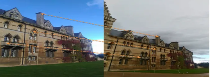
![Figure 3.7: Examples of RGB-D images: Texture vs Color [84]. (a), and (b) are images taken from an environment where the geometric measurements are more significant than photometric measurements while (c), and (d) were taken from a scenario where the textu](https://thumb-eu.123doks.com/thumbv2/123doknet/13140354.388579/55.918.260.659.225.951/examples-texture-environment-geometric-measurements-significant-photometric-measurements.webp)
Documents relatifs
This paper presents a robust real time 3D pose and orienta- tion estimation method based on the tracking of a piecewise planar object using robust homographies estimation for vi-
To cope with all these problems, we propose a model based pose estimation method for depth cameras composed of three stages: The first one uses a probabilistic occupancy grid
In the second, recognition stage, an action recognition approach is developed and stacked on top of the 3D pose estimator in a unified framework, where the estimated 3D poses are
Figure 1, illustrates a general instance of a finite length crack tip segment undergoing a clockwise rotation, in turn subjecting the elements in the vicinity to changes in
Key words: crack propagation, interacting cracks, energy release rate, extended finite element method, linear elasticity, energy minimisation.. In computational fracture mechanics
• Energy release rate w.r.t crack increment direction:.. • The rates of the energy release rate are
FF 8) Reprendre la question I.7 en ne supposant plus les annuités constantes : tant que le prêt à taux 0 n’est pas remboursé, les 650 e de remboursement sont partagés entre
In the mK range, somewhat larger effects, such as the ultralow T plateau [8] of the dielectric constant, and the internal friction behavior [9], were ascribed to TLS interactions..
