HAL Id: hal-03002474
https://hal.archives-ouvertes.fr/hal-03002474
Submitted on 5 Feb 2021
HAL is a multi-disciplinary open access
archive for the deposit and dissemination of
sci-entific research documents, whether they are
pub-lished or not. The documents may come from
teaching and research institutions in France or
abroad, or from public or private research centers.
L’archive ouverte pluridisciplinaire HAL, est
destinée au dépôt et à la diffusion de documents
scientifiques de niveau recherche, publiés ou non,
émanant des établissements d’enseignement et de
recherche français ou étrangers, des laboratoires
publics ou privés.
Sedimentary record of rapid climatic variability in the
North Atlantic Ocean during the Last Glacial Cycle
Elsa Cortijo, Pascal Yiou, Laurent Labeyrie, Michael Cremer
To cite this version:
Elsa Cortijo, Pascal Yiou, Laurent Labeyrie, Michael Cremer. Sedimentary record of rapid climatic
variability in the North Atlantic Ocean during the Last Glacial Cycle. Paleoceanography, American
Geophysical Union, 1995, 10 (5), pp.911-926. �10.1029/95PA02021�. �hal-03002474�
PALEOCEANOGRAPHY, VOL. 10, NO. 5, PAGES 911-926, OCTOBER 1995
Sedimentary record of rapid climatic variability in the North
Atlantic Ocean during the last glacial cycle
Elsa
Cortijo,
• Pascal
Yiou,
2 Laurent
Labeyrie,
•'3
and
Michel
Cremer
4
Abstract. Comparisons
between
a Greenland
ice core isotopic
record
and marine
sediment
grey
level records
of the North Atlantic
Ocean
show
that rapid
temperature
variations
witnessed
by the
ice core (Dansgaard-Oeschger
events)
during
the last glacial
period can also be detected
in marine
sediments.
This shows
that the resolution
obtained
in marine cores
can be sufficiently
high to
record
rapid climatic
fluctuations.
Several
spectral
analyses
of those
grey level marine
records
consistently
indicate
that significative
fluctuations
of the climatic
response
exist with periodicities
of 5 to 1 kyr in addition
to orbital forcing.
These
high frequencies
are close
to those
predicted
by
various dynamic ocean models.
Introduction
The climatic system is clearly recognized to be continually variable, on all timescales [Mitchell, 1976]. Many different
physical processes can contribute to climatic variability on one or another timescale. Climatic variance on the orbital timescale [Hays et al., 1976] is centered around periodicities of
100, 40, and 20 kyr (100 kyr corresponds to the dominant
periodicity of middle-late Quaternary glaciations; 40 and 20 kyr are associated with variations of obliquity and precession of the Earth, respectively). Orbital changes in insolation were gradual and occurred over several thousand years. However, there is now abundant evidence for climatic changes on
millenial timescales which cannot be accounted for only by
orbital variations and must be explained also by internal oscillations of the system or interactions between the orbital forcing and internal mechanisms. Ice core records obtained in
central Greenland reveal that the last glacial period was
extremely unstable [Dansgaard et al., 1982; Greenland Ice core Project (GRIP) Members, 1993]. Those large and abrupt
climatic transitions, the Dansgaard-Oeschger events, lasted a
few decades. Such high-frequency oscillations were also
detected in the deuterium isotope profile (fiD) of the Vostok ice
core [Yiou et al., 1994]. The oceanic signal has usually been considered to be too rough to detect such variability because of the bioturbation effects. The postdepositional mixing of sediment layers by biological activity, the bioturbation effect,
•Centre des Faibles Radioactivit6s,
Laboratoire mixte
CNRS/CEA, Gif-sur-Yvette, France.2Laboratoire de Mod61isation du Climat et de
l'Environnement, CEA, Gif-sur-Yvette, France.
3Also
at D6partement
des
Sciences
de la Terre, Universit6
de
Paris-Sud/Orsay, Orsay, France.
4D6partement
de G6ologie
et d'Oc6anographie,
Universit6
de
Bordeaux 1, Talenee, France.
Copyright
1995 by the American
Geophysical
Union.
Paper number 95PA02021.
0883-8305/95/95 PA-02021 $10.00
tends to smooth the rapid climatic events but does not
completely remove them as shown here. In North Atlantic cores
above 40øN, the continual mixing of the sediment by benthie activity is estimated to be less than 5 cm [Griggs et al., 1969].
Another modification in the sediment can be due to occasional large burrows which transport sediment into lower levels. This
kind of bioturbation can easily be identified during the treatment of the core. Hence the purpose of our paper is to determine the high-frequency part of the climatic variability contained in marine sediments. First, we compare marine sediment and ice core records. Second, we conduct spectral
analyses of marine sediment records. We show that marine
sediments can detect rapid variations of the climatic system down to periods of 1.5 kyr. Some of these variations may be global, but others are specific to the North Atlantic in relation
with Greenland.
Material and Method for Measurements
of Sedimentary Reflectance
We selected cores from 10 sites in the North Atlantic Ocean located between 41 ø and 60 ø N and between 20 ø and 30 ø W
(Table 1 and Figure 1). Cores were taken from various depths of each side of the Mid-Atlantic Ridge above the carbonate
compensation depth. In all cores, the grey reflectance of surface
sediment was measured following the method developed by
Bond et al. [1992a].
The cores were digitized by sections of 75 cm in length with
a tri-CCD (Charged Coupled Device) color camera. The
lighting is constituted by two neon glow lamps. For each core,
we obtain an image by concatenation of all of the 75-cm
sections. In this image, one pixel represents approximately 1.3
xrm of sediment. The theoretical temporal resolution lies between 20 and 100 years (depending on the sedimentation
rate). The intensity of reflected light is expressed as a color
level: red, green, or blue level. The signal thus obtained is expressed in a conventional scale varying between 0 (black) and 255 (red, green, or blue). To reduce the initial length of the data series (close to 16,000 points), the raw color level reflectance data were smoothed by a least squares method and interpolated every 5 mnx The new series contains
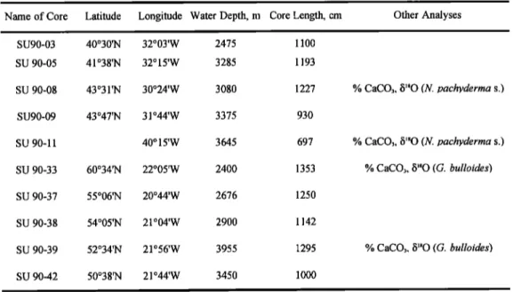
Table 1. Location of Cores Used in This Work and Available Analyses
Name of Core Latitude Longitude Water Depth, m Core Length, cm Other Analyses SU90-03 40ø302q 32ø0YW 2475 1100
SU 90-05 41ø382q 32ø15'W 3285 1193
SU 90-08 43ø3 I'N 30ø24'W 3080 1227 % CaCO,, 8180 (N. pachyderma s.)
SU90-09 43ø47'N 31ø44'W 3375 930 SU 90-11 40ø 15'W 3645 697 % CaCO,, 8180 (N. pachyderrna s.) SU 90-33 60ø342q 22ø05'W 2400 1353 % CaCO,, 8180 (G. bulloides) SU 90-37 55ø06'N 20ø44'W 2676 1250 SU 90-38 54ø05'N 21ø04'W 2900 1142 SU 90-39 52ø34'N 21ø56'W 3955 1295 % CaCO•, •5'•0 (G. bulloides) SU 90-42 50ø38'N 21ø44'W 3450 1000
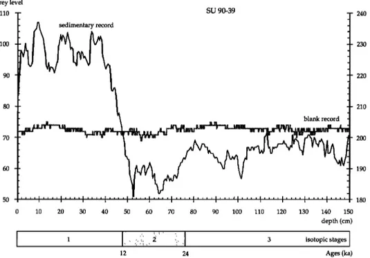
approximately 2500 data points. The difference between raw and smoothed interpolated reflectance curves is smaller than 2%. Thus this process has hardly any effect on the original signal. Lighting conditions are homogeneous fi'om top to bottom for a section of a core and fi'om core to core. There is negligible illumination distortion in the digitized image: the reference curve (a white ruler) has a distortion of about 1% of the total scale which corresponds to about 3-4% of the mean signal in the North Atlantic (Figure 2).
Validity of the Reflectance Signal
for Paleoclimatic Reconstructions
In order to document the paleoclimatic validity of this method, we examined the sedimentological parameters of the
cores. Marine sediments in the North Atlantic contain three principal components: biogenical carbonate, detrital elements, and, in some areas, volcanic ash [Ruddiman and Glover, 1972; Smythe et al., 1985]. The most important color variations are due to variations in the biogenic carbonate content, which is highly correlated with climatic variations [Crowley, 1983], because their development is seasonal and driven by annual fluctuations of surface water temperature. The Coccolithophoridae (carbonated nannoplankton) and foraminifera are abundant when the water temperature is warm. Consequently, the sediment deposited during those periods is white. During glacial times, the sediment deposited is rich in
detrital particles (clay minerals or coarse particles) originating
from the continent and transported by bottom currents or ice
-75 -65 -55 -45 -35 -25 -15 -5 5 15 70 70 6O 5O 4O -75 -65 -55 -45 -35 -25 - 15 -5 5 60 50 40 15
CORTIJO ET AL.: SEDIMENTARY RECORD OF RAPID CLIMATIC VARIABILITY 913 grey level 110 su 90-39 240 lOO 230 90 220 80 210
I ...
.•_._•_•
... \
blank
record
-[
70 200 60 190 50 180 0 10 20 30 40 50 60 70 80 90 100 110 120 130 140 150 depth (cm)I
I
if.• I
3
isotopic
stages
]
12 24 Ages (ka)
Figure 2. Grey level record of the first section of core SU90-39 compared to the blank record. The thick curve i s
the blank record with the right scale, and the thin curve is the reflectance profile with the left scale. Isotopic
stages are indicated with the transition ages.
rafting. The sediment is therefore dark. Bond et al. [1992a] have shown that the sediment reflectance is well correlated with fluctuations of Neogloboquadrina pachyderma s. (polar foraminifera) and confirm that reflectance is a good indicator of climatic variations. Ash layers are characterized by dark level (about 80 in our conventional scale) which is not related to
glacial
periods.
Around
volcanic
areas,
the climatic
signal is
altered by the layers left by volcanic eruptions. Thus we didnot use cores located around the Azores or Iceland for this
study. In the cores we used for this study, the sediment is made up of foraminifera and clays. We selected cores not perturbated
by turbiditic processes.
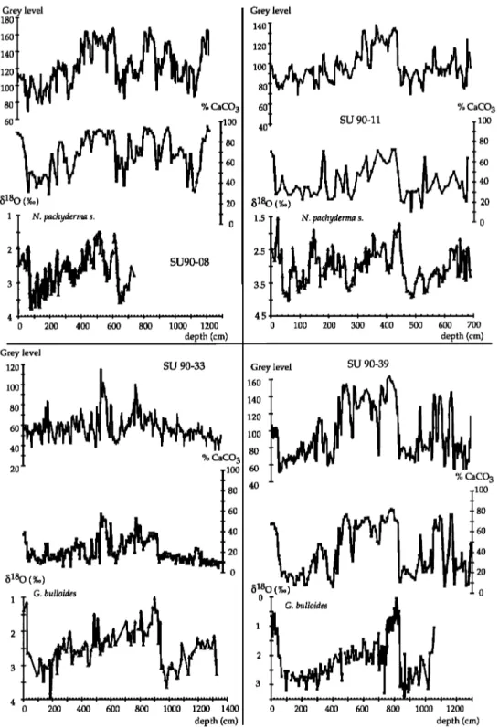
We made regressions between carbonate content (measured by a gasometric technique with a precision of 1%) and reflectance on four of the cores (Table 1). The reflectance, carbonate content, and isotope data are shown in Figure 3, and
the correlations between each colour channel and the carbonate percentage are shown in Figure 4. The correlation coefficients
are 0.864 for the red channel, 0.881 for the green channel, and 0.905 for the blue channel after removing the upper few ten of centimeters of the core which are noticeably offset fi'om the
correlation lines. This is due to red coloration of the sediment
by iron and manganese oxides. This represents a limit of this method because the most recent part of the sediment is always
too dark. The best correlation with CaCO3 is obtained with the
green and blue channels. We chose to use the green channel because the blue signal is more affected by the polarizing filter used to decrease direct reflection. In this paper, we will use the
term "grey level" to indicate the green channel variations. The oxygen isotopic composition of planktonic foraminifera
expressed as relative b180 (permil versus peedee belemnite (PDB) standard) was measured in the four cores (Table 1 and
Figure 3). This signal depends directly on changes in ice volume, surface water temperature, and salinity [Emiliani, 1955; Shackleton and Opdyke, 1973]. The sampling was made every 5 cm on average. The species analyzed are Globigerina bulloides and/or N. pachyderma left coiling. We compared planktonic isotopic data with sediment reflectance in the same cores. Figure 5 shows this comparison in core SU 90-08. During most of the record, the sedimentary reflectance exhibits the well-known large glacial-interglacial variations. For large timescales, the two signals are in agreement except during rapid events of the last glacial period. The rapid variability during
this time is now clearly identified as Heinrich events
[Heinrich, 1988; Broecker et al., 1992]. They correspond to the melting of great quantities of icebergs, bringing freshwater (isotopically light) into the surface of the North Atlantic and lithic particles into the sediment. Isotopically, they appear as light peaks of/5•80, and they are characterized by a globally synchronous dark level in the reflectance data [Bond et al., 1993], but this dark level is interspersed with light shifts perhaps due to the occurence of detrital carbonate levels [Bond
et al., 1992b].
In the North Atlantic Ocean, outside the volcanic areas, we
can therefore use grey level values as a first-order stratigraphic tool (Figure 6) when the variations in the carbonate contents are large (oscillation areas of the polar and subtropical front).
Comparison Between Grey Level
Measurements and Ice Core Records
Foraminiferal abundance and/5•80 changes reflect, at least in
part, the rapid temperature changes of the air above Greenland during the Dansgaard/Oeschger events [Bond et al., 1993].
Grey level 180' 160' 140' 120' 100' 80 % CaCO 3
60
l100
80 60 40 20 N. pachyderma s. 0 SU90-08 ''"C .... : .... : .... : .... : .... : .... : .... : ... : 0 200 400 600 800 1000 1200 depth (crn) Grey level 140 120 100 80 60 % CaCO 3 SU 90-11 100 4C 818O(%o) 1 Grey level120
•
SU
90-33
100
I
80 60ø
1oo
80 6o 4o 20 o 5180 (Ooo 1 2 3 ... 0 200 400 600 800 1000 1200 1400 depth (arn) 8O •5180 (%o) 20 N. pachyderma s. 0 1 2 3 0 1•0 21•0 3•)0 4•0 5•0 6/30 7150 depth (am)Grey
level
SU 90-39
160 140 120 100 80 60 % CaCO 3 40 .100 80 60 40 20a108
0
0 200 400 600 800 1000 1200 depth (am)Figure 3. Comparison between grey level, carbonate content, and isotopic •5•80 on four cores versus depth in
the core.
This confirms the strong coupling of the northern Atlantic Ocean with the atmosphere-ice system predicted by various dynamical models [Peltlet, 1992]. Because the ice core isotopic records indicate large variability in the 0.5 - 2 kyr range of
duration
[dohnsen
et al., 1992], we test the validity of the
sedimentary reflectance signal by direct comparison between the Greenland ice core (GRIP)and sedimentary records.Measurements of •5•80 in the GRIP core provide a proxy for the variations of air temperature over the ice cap with a very high
temporal resolution [Dansgaard et al., 1993].
The comparison between the grey level and the GRIP ice core records is shown in Figure 7. The changes between dark
and light levels are separated by sharp boundaries and
CORTIJO ET AL.: SEDIMENTARY RECORD OF RAPID CLIMATIC VARIABILITY 915 Grey level 2OO 160 120 80 40
*•**•*••t
"$'ß
'
Red
channel
ß
y= 1.3'x
+ 47.77
r2=0.86 200 -160
.
80
'••-•-•-
*
Green
ch•el
40
.
y=l.29*x+36.93
r2=0.88
0 I I I I I I I I I 2OO 160 120 80 40 0 10 20 30 40 50 60 70 80 90 100 Carbonate content (%)Figure 4. Regression between grey level and CaCO.• measurements in four cores for the red, green, and blue
channels. Equations of correlation lines and correlation coefficients are indicated for each color channel. The significance level of this correlation coefficient is 95%.
would, on the contrary, smooth the signal. In addition, in order
to remove most of the perturbations from the record, we use an
algorithm based on pattern recognition. The digitized color image of the core is, at each depth, about 64 pixels wide, corresponding to the 10-cm width of the core. A rough solution would be to simply choose a "good" profile among these 64 possibilities or to take the mean. Alternatively, the algorithm used here, derived fi'om vocal analyses, tries to find coherent patterns along the core depth and rejects all other
pixels. Using the whole width of the core, this filter thus removes most of the local perturbations, such as burrows,
provided that they are smaller than the core width. Unlike classical time series filters, this method preserves high frequencies by using most of the information contained in the original two-dimensional color image.
We used the numbering of the interstadial events of the GRIP ice core [GRIP Members, 1993; Dansgaard et at., 1993; Grootes et at., 1993] between 20 and 110 ka. The duration of interstadials lies between 0.5 and 2 kyr [dohnsen et at., 1992]. Cores located between 50 ø and 60 ø N and 25 ø and 15 ø W
(SU90-38, SU90-39) show a good correlation with the GRIP
Grey level 170 - 150 - 130 - 110 - 90- 70 50 30
õ180
(%o),
N. pachyderma
s.
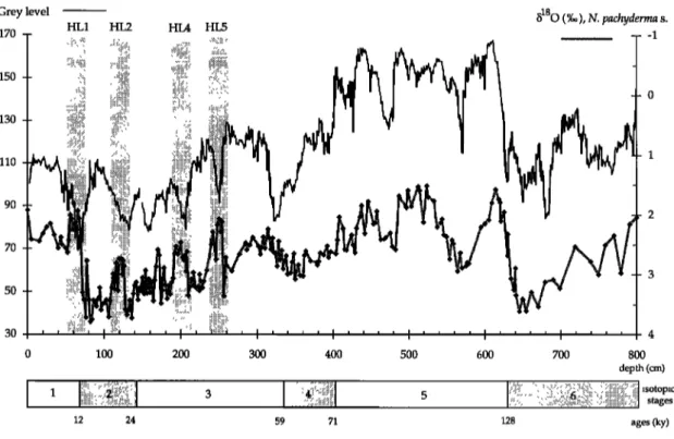
HL1 HL2 HL4 HL5 1 3 ' ' ' I .... I .... I ' ' I 4 0 100 200 300 400 500 600 700 800 depth (cm) stages 12 24 59 71 128 ages (ky)Figure 5. Comparison between isotopic 5180 record of N. pachyderma s. (diamonds) and the grey level record of
core SU90-08. Heinrich layers have been underlined. We can see that the Heinrich layers are characterized by dark levels and light isotopic peaks. This corresponds to the discharge of a great quantity of icebergs which give freshwater melting and dark detrital material.
interglacial [Dansgaard et al., 1993; McManus et al., 1994; Corto'o et al., 1994]. During glacial periods, the Dansgaard- Oeschger events found in the ice may also be clearly observed in marine sediments as small reflectance changes with an amplitude of 10 units or more. These small variations, which last about 1.5 - 2.0 kyr, are indeed very often common to marine sediments and the ice core. During the transition between
isotopic stages 5 and 4, all records (marine and ice) have the same pattern. There is an excellent agreement between proxy
data for high-latitude temperatures and the marine sediment
record. This transition (isotopic stages 5-4) is achieved in several steps, suggesting abrupt changes in atmospheric and
thermohaline circulations. These cores are sensitive to Gulf
Stream variations and to the associated heat transport. These results are in agreement with those of Keigwin and Jones
[1994].
On the other hand, the cores located between 35 ø and 45 ø N
and 30 ø and 40 ø W (SU90-08, SU90-05) do not show as good a correlation with the Greenland record for rapid variability, although we easily recognize the successions of glacial- interglacial periods. This can be due to some smoothing effect
of the climatic system which weakens the effects of the events
initiated in the North Atlantic as they are transported toward the south. Another possibility is that the rapid oscillations are due to Gulf Stream variations which are well marked only in area of climatic front oscillations (polar or subpolar front).
Variability of the Grey Level Records
in the Frequency Domain
Several sediment core studies have identified significant high frequencies in paleoclimate proxy data [Pisias et al., 1973; Pestiaux et al., 1988]. Due to their very fine temporal resolution, reflectance records are appropriate to test the periodicities of the suborbital timescale. We chose two specific cores to perform several detailed spectral analyses. Each of them is representative of an area of the North Atlantic (Table 2). Core SU90-08 (Figure 1) is located in the southern boundary of the polar front oscillation [Climate.' Long-Range Investigation, Mapping, and Prediction (CLIMAP) Project Members, 1984]. Core SU90-39 (Figure 1) is located in the northern boundary of this area (area of maximum of oscillation).
Chronology
We developed a timescale for each site based on accelerator
mass
spectrometry
(AMS)
•4C
dates
(until
30 ka),
benthic
and
planktonic •80, and the Spectral Mapping (SPECMAP) stack
[Pisias et al., 1984]. In core SU90-08, the sampling resolution of benthic and planktonic foraminifera signals is 2 cm for 0-128
kyr and 5 cm for 128-285 kyr (for planctonic foraminifera only).
In the uppermost
portion
of the record,
the •4C
available
data
CORTIJO ET AL.' SEDIMENTARY RECORD OF RAPID CLIMATIC VARIABILITY 917 0 24 59 71 128 183 Age (ky) 180 1 I I I I I • iiiiiiiii!i' SU 90-37 55øN 20øW 20 1 '• :-- ...-...- 18o .' . -...-' ,.' .-' 54øN 21øW 20 •8o : : . '-.. '.. 40 180 50øN 21øW 2O 180 ' SU 90-09 43øN 31øW
•
...
43øN
30øW
t50 ß ß ß "~. 18080 ...
.'".."'
.-''"'
... ...
200,
,-0.5 18
0 (%o)
(G.
bulloikl.
es)
'
.
.
1.5 SU 90-08 43øN 30øW ! i i i ½) 200 400 600 800 1000 1200 depth (cm) 12 24 59 71 128 183 245 Age (ky) SU 90-05 41øN 32øW
shifted by 3 m to the left
SU 90-03
40øN 32øW
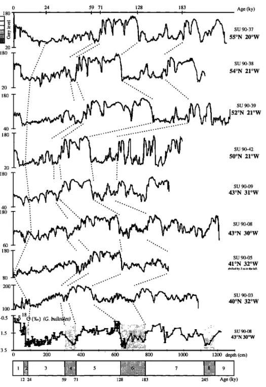
Figure 6. Correlation between several cores in the Norlh Atlantic Ocean and the /5•80 record of Globigerina bulloides in core SU90-08 (age scale at bottom). Glacial periods are dashed. The age scale at the top
corresponds to core SU90-37.
the software AnalySeries [Paillard, 1995a]. Between the stratigraphic correlation levels, the sedimentation rate is assumed to be constant and a linear interpolation was applied. In core SU90-39, the sampling resolution is more irregular, varying between 2 cm and 10 cm. The SPECMAP chronology was applied in this case too. The age-depth relation for the two
cores is shown in Figure 8. We make no claim that our stratigraphies are the most accurate, but they are built using all available classical stratigraphic signals. The theoretical sampling lies between 20 and 50 years. The corresponding mean Nyquist period (the theoretically shortest period) and the
0 10 20 30 40 50 60 70 80 90 100 110 120 -40 b • o (%.) -44
180 Grey
level
2o
100
60
i:i:• :i:!: i:i:i
20 H4 H5 H6 160 120 8O 4O Ages (ka)
180
T
:
ß 140 100 180 6O 140 100 • 60 0 100 200 300 400 500 600 700 Depth (cm) "l. •' ... '<Wo•'•":••••qi•i.."•il s, ss s, sa I Isotopic stagesFigure 7. Correlation
between
the GRIP (Greenland
Ice core Project) record
versus
age [Dansgaard et al.,
1993] and the sedimentary
grey level of the North Atlantic
cores.
These
grey level records
are obtained
using a
filter which removes
all pertubations
in the stratigraphy.
All North Atlantic cores
were put on the same
depth
scale.
The numbering
corresponds
to the interstadial
events
of the ice and has been used for marine
cores as
well.
However, the sedimentation rate is not constant along a given core; this implies a variable time step and a variable Nyquist period.
Spectral Methods
The study of the orbital components and the high-frequency variability on those time series was made with several spectral methods. Each of them examines a particular feature in a time series, and combining those different spectral analyses permits
avoiding
spurious
results
and thus enhances
the confidence
of
our estimates. The techniques used are multitaper method and wavelet transform. We also use singular spectrum analysis in order to separate the signal and the noise. Then we can analyze the high-frequency variations.
Multitaper method. The purpose of this nonparametric
spectral
method [Thomson,
1982] is to compute
a set of
independent
and significant
estimates
of the power
spectrum,
in
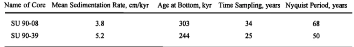
CORTIJO ET AL.: SEDIMENTARY RECORD OF RAPID CLIMATIC VARIABILITY 919 Table 2. Sedimentation Rate and Nyquist Frequency of Cores Used in the Spectral Analysis
Name of Core Mean Sedimentation Rate, cm/kyr Age at Bottom, kyr Time Sampling, years Nyquist Period, years
SU 90-08 3.8 303 34 68 SU 90-39 5.2 244 25 50 Age (ky) 300 -- 250 2OO 150 100 - 50 ! ! core SU90-08 i i i i i I 0 200 400 600 800 1000 Age (ky) 300 - - 250 - - 2OO 150 100 50 1200 1400 depth (cm) core SU90-39 ' ' ' ' I ' ' ' ' I ' ' ' ' I .... I .... I .... I .... 0 200 400 600 800 1000 1200 1400 depth(cm)
Figure 8. Age-depth relation for the two studied cores: (top) core SU90-08 and (bottom) core SU90-39. The sedimentation rate is relatively regular in the two cores except during stage 6 (around 160 kyr) of core SU90-
109.22 39.96 4.68 3.92 • • • 3.44 2.28 20• :' • 7.31 • •0.99 6 0.99
?: 19.73
/•
'i [
• 15
-I-
[1 ii /]"
i
:i
• 0.98 2
0.98
< 10 } , ',, 0.97 8 0.97 5 ',, ,, • ,, 0.96 .4 0.96 ,,', :,, • ',', 0 , .- , ... -. , 0.95 0 ... 0.95 0 0.05 0.1 0.15 0.2 0.25 0.25 0.3 0.35 0.4 0.45 0.5 1.6 1.2 0.8 0.4 o 1.98 1.75 1.33 1.28 1.03• 1.88 ] 1.70
•
• 1.26
'""1', ,
; i•
'
' '1.2o
.:,, ,•,
,'
:: ••
::. ,
....-:: i!
:: :!
i!
"'
I I II?
'
ß::
II ,, , .... ,,• I I r, ' '! ' ' ' ' ' ' i • ß ß ., ., , ,. • , , , ,. 0.5 0.55 0.6 0.65 0.7 0.75 0.8 0.85 0.9 0.95 Frequ•cy (•cle/ky) 0.99 0.98 0.97 0.96 0.95 1b
117.02 2.3425
T aq'
39
7.65
T 1
2 T
3.36
/• 2.22
½
23.40
½
i [ ½
2.•6 '
• llil • " 12.90
+ i
/
•
:' •
=•5
]1••
.••
'] • • •{
] 0.98
• •.2
<1o -
ii
0.97 0.8
5
,
ii
I
i o.• o.•
o
0 0.05 0.1 0.15 0.2 0.25o
0.25... ,...,,..,..
0.3 0.35 0.4 0.45 0.99 0.98 0.97 0.96 0.95 0.5 1.6 1.2 0.8 0.4 o 0.5 1.07 /• 1.01137
1.17
•
i: •, T •
'
•.
-
•.•3
!
':: :! ;o.•
• ,,: ; ,,, • :l 1: :,, 0.98!•
"
0.97O.96
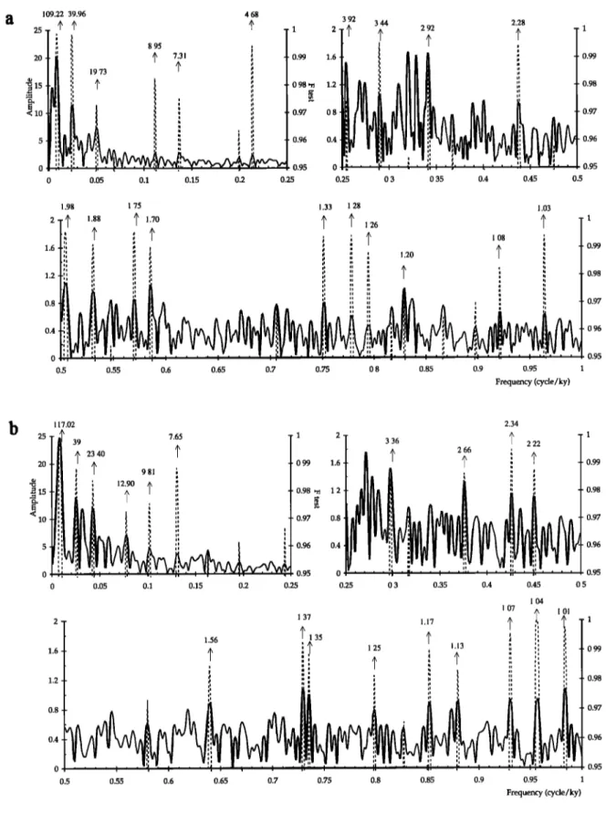
, -, .... ß ... 0.95 0.55 0.6 0.65 0.7 0.75 0.8 0.85 0.9 0.95 1 Frequency (cycle/ky)Figure 9. MTM (multitaper
method)
spectra
of raw grey level on cores
(a) SU90-08 and (b) SU90-39. The solid
line represents the line amplitudes, and the dotted line represents the F test of estimate confidence. For a better representation, the frequency range 0-1 has been divided into three panels. The significative periodicities have
CORTIJO ET AL.' SEDIMENTARY RECORD OF RAPID CLIMATIC VARIABILITY 921
single-taper methods given a finite and possibly short time [Vautard et al., 1992]. The harmonic analysis estimates series. A set of optimal tapers is calculated so that this provide a statistical test (Fisher or F test) for the amplitude approach to spectral estimation is less heuristic than spectrum. High values of this test allow rejection of the null traditional (e.g., Blackman-Tukey) techniques. The tapers are hypothesis of a nonperiodic component at some frequency. calculated to optimize the spectral leakage due (to the data One of the main assumptions of this technique of harmonic finiteness) outside a prescribed bandwidth W, for a periodic analysis is that the signal must yield periodic and separated signal [Thomson, 1982]. The number of relevant tapers is then components. If not, a continuous spectrum (in the case of a
proportional to the bandwidth [Slepian, 1978], so that a
colored noise or a chaotic system)will be broken down to
tradeoff
between resolution (small W) and confidence
(large
spurious
lines with arbitrary
frequencies
and possibly high F
number of tapers) has to be found, by trial and error or other values. This is a danger of the method, which can be partiallyheuristic criteria [Thomson, 1982]. avoided if the raw power spectrum is computed and hints for
Thus, with a set of Ktapers with a given bandwidth W, K lines are detected; it is also very important to vary the
independent
spectral
estimates
can be computed
for a time
bandwidth
parameter
W and
the number
of tapers
to ensure
the
series X, from the product of X and each taper. An average over stability of the frequency and module estimates.
these spectra gives a multitaper spectral estimate which Singular Spectrum Analysis. Singular spectrum analysis possesses good statistical properties [Thomson, 1982]. (SSA hereafter)takes its roots in digital signal processing and Multitaper methods (MTM hereafter) are also useful to nonlinear dynamics [Broomhead and King, 1986; Vautard compute the harmonic analysis of a time series, i.e., to determine and Ghil, 1989]. It is designed to extract information from short the amplitude and frequency of its line components. This is and noisy time series, without prior knowledge of the done through a least squares regression in the frequency dynamics of the underlying system that generated the series. domain. Under white noise hypotheses, the amplitude and line The st. arting point of the method is to embed a time series of frequency estimates are unbiased [Lindberg, 1986], and they observables X(t), t = 1... N in a vector space of dimension M.
are robust to such hypotheses when a red noise is used The embedding procedure consists of constructing a sequence
100000 10000 1000 100 10 PC1-4 I i i i PC5-15 i i i , i I .... 0 5 10 su90-08 15 20 25 30 35 40 Order (k) 100000 PC1-4 10000
1000
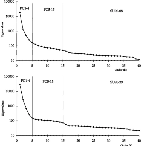
100 10 ,''''• PC5-15 SU90-39 0 5 10 15 20 25 30 35 40 Order (k)Figure 10. Singular spectrum analysis (SSA) eigenvalues of grey level of cores SU90-08 and SU90-39. The
E of M-dimensional vectors of delayed coordinates from the
time series X
•(t) = (X(t), X(t+ 1) ... X(t+ M-1)), t= 1... N- M + 1.
If the system
dimension
d is relatively small (d < 3), such a
procedure
can give a stunning reconstruction
of the system
attractor
[Gershenfeld,
1988]. On the other hand, if d is larger
than four, a raw application
of this technique
fills any two-
dimensional
projection in a dense way so that no visual
information
can be retrieved.
SSA allows unravelling
of the
information
entangled
in the delayed-coordinate
phase
space
by decomposing
the sequence
of vectors E into elementary
oscillation patterns. Hence this method generates data-
adaptative filters for the separation of the time series into
independent
components,
like trend, deterministic
oscillations,
and noise.The directions of extension of the sequence of
augmented vectors •(t) are determined. An M x M covariancematrix
ofX, CX, is computed,
as well as its eigen
elements
(•k,
pk),k = 1 ... MThe eigenvalues •k give the extension of the time series in the
direction
given
by the (orthogonal)
eigenvectors
Pk: the •k are
associated
to the variance
of the oscillating
pattern
detected
by
the Pk. Therefore
plots of the sorted eigenvalues allow
discrimination
between
high variance
oscillations
with steep
slope and noise characterized by low values and a flat floor [Vautard and Ghil, 1989]. Projections of the time series onto
the eigenvectors
yield the principal
components
(PCs) a k
A time series associated to a single or several eigenvectors Pk can be reconstructed by combining the associated principal
components M
r^(t)
=
1__
Mtk• • ak(t-i)pk(i),
i=1 Mak(t)=• X(t+i)pk(i).
i=1 Grey level 200 SU90-08160
120
80 0 . : I ' I I ' I ' ' ' ' 0 50 100 150 200 250where
A is the set of empirical
orthogonal
functions
(EOFs) on
which the reconstruction is based and Mt is a normalization
factor [Vautard et al., 1992]. This reconstruction
process
preserves the phase of the time series, so that X and r A can be
superimposed on the same timescale. Once the noise and trend
components are identified by SSA decomposition, a clean signal can be reconstructed and analyzed, pattern-wise or with
other mathematical tools.
Wavelets. Most observational signals are not stationary and contain transient components which excite a wide range of
frequency in a limited amount of time. This motivates the use of time-frequency representations and wavelet transforms.
Applications of wavelet transforms have been extensively reviewed by Grossmann et al. [1989] and Farge [1992].
The main property of a wavelet decomposition is that the analyzing functions (the wavelet functions) are localized both
in time and frequency, i.e., they oscillate in a finite amount of time and vanish, as well as their Fourier transform. On the
opposite, the sine and cosine functions (of Fourier transforms) are perfectly localized in frequency but oscillate endlessly in time. Hence a classic Fourier analysis spreads the singularities of a time series over the entire power spectrum, creating
spurious peaks or concealing real ones, unless an ad hoc time-
frequency analysis is performed, such as by Yiou et al. [1991 ] or Birchfield and Ghil [1993]. As a wavelet decomposition only uses dilatations and translations of a unique function, it is optimal in the sense of the so-called time-frequency
27O 23O 190 150 110 7O 3OO 2OO 160 120 40 SU90-39
i
,
;
t
,: I
.
i ' 'I ' • • • I 50 100 150 2• 250 60 3OO Age (ky) 260 22O 180 140 100Figure 11. Raw grey level of cores
(top) SU90-08
and (bottom)
SU90-39 with the corresponding
reconstructions.
For the two cores,
the raw grey level is the thin dotted curve,
PC1-4 is the solid thick curve
CORTIJO ET AL.: SEDIMENTARY RECORD OF RAPID CLIMATIC VARIABILITY 923
uncertainty principle [Farge, 1992], in that the correlation between duration and average frequency is respected.
A wavelet analysis decomposes a time series into scale components, hence allowing a discrimination between oscillations occurring at fast (time) scales and others at slow scales. More precisely, for some signal X and a given wavelet function •, the • wavelet transform of X, at a scale a and a time
b, is given by
=
1 I••(t3)x(t)dt.
W•,X(a,b)
•aa
.
This integral expresses an analysis of X, localized around b and
scaled by the parameter
a. The wavelet decomposition
is
represented
in a dilatation (scale)-translation
(time) plane. A
logarithmic scale axis allows for a better resolution of small-scale components, i.e., high frequencies.
In the case
of a purely monochromatic
signal
X(t)= ,,1 exp(i
to o t), the wavelet transform isWw X(a,b) = A a r ..• i mnb
2•
where
• is the Fourier
transform
of •. From
this relation,
the
modulus of W, X does not depend on the translation time b,
and the phase of the wavelet transform
at a scale a directly
gives toO. This means that in such a representation, the wavelet transform of a purely periodic signal is a ridge at a constant
scale [Farge, 1992].
In this paper, we use the complex Morlet wavelet
W(t)
= exp(2
i p too
t) exp(-t2/2)
+ negligible
correction
terms,
i.e., a complex exponential modulated by a Gaussian function.We truncated the sides of the wavelet transforms to avoid spurious side effects.
Results of Spectral Analyses and Discussion
In the two cores (SU90-08 and SU90-39), the grey level records are investigated with MTM harmonic analysis. MTM results are shown in Figures 9a (core SU90-08) and 9b (core SU90-39). In the following discussion, we will only consider
peaks with confidence
tests (normalized
statistical F test)
greater than 0.97.Frequencies associated with orbital parameters (precession and obliquity) are well defined in both cores with high values of amplitude (between 8 and 25). High frequencies have much smaller values of amplitude. Some of these periodicities were detected in other works: Hagelberg et al. [1994] and Yiou et al. [1994] have observed "submilankovitch" periodicities between 10 and 12 kyr. They correspond to variability which can be attributed to internal climatic system, nonlinearly coupled to precession forcing [Hagelberg et al., 1994]. The periodicities between 1/5 and 1/8 cycle per kyr exist in the two cores and could be related to Heinrich events. They have also been found in ice core records [Yiou et al., 1995], and it can be speculated that these oscillations are symptomatic of the succession of rapid oscillations during the glacial period. SSA analyses allow us to determine which is the part of the noise in the grey level signal. Singular spectra are obtained by taking
an embedding dimension of 40 (time sampling is 0.5 kyr and the window size represents 20 kyr) and are presented in Figure 10. In both cores, the spectra can be separated in three disctinct regions: the first part (PC1-4) with a steep slope dominated by the large glacial-interglacial variations (linked to orbital frequencies), an intermediate region with a more gentle slope (PC5-15) which contains high-frequency variations, and the final noisy region. The reconstruction of the principal components is shown in Figure 11. Spectral analyses made on these reconstructions show that the frequencies detected by the
MTM method are real and not linked to noise.
Because of its temporal resolution, sedimentary reflectance provides detailed information in the higher frequencies. Between 1/4 and 1/1 cycle per kyr, both cores present significative periodicities although they are not exactly the same. These results confirm that marine sediments can record high-frequency climatic oscillations.
We could identify some oscillations with MTM analyses, but this method does not give information about the
stationariness of the features we find. In order to study how
those different periodicities evolve in time, we use a wavelet
analysis on both cores. However, the low and high frequencies
determined by MTM analysis in the two cores are not stationary, and no perfectly stationary components are detected. This is also the case for ice core records [Yiou et al.,
1995] which do not show any stationary frequency.
However, the wavelet representation of core SU90-39 shows many similarities with the ones obtained for the GRIP record, although it is relatively different from the ones obtained in core SU90-08 (Figure 12). This is in agreement with the qualitative observation made by direct comparison between the SU90-39
grey level and the GRIP/5•80 record.
The two cores show nonstationary suborbital periodicities between 5 and 1 kyr. Several simple climatic models [Welander, 1982], and also some more complex models, like two-dimensional ones [Hovine, 1993], have shown oscillations. The conceptual salt oscillator climate model [Broecker et al., 1990; Birchfield and Broecker, 1990] fluctuates between an "on" (the northern hemisphere is relatively warm because of the large transport of heat to high latitudes) and "off' mode (the northern hemisphere is cold, a consequence of the greatly reduced thermohaline circulation) with a period of the order of 1 kyr. But those oscillations are not spontaneous; they are forced by external freshwater input. This model emphasizes the role of salt fluxes and their control of density gradient. Other simple models present spontaneous
oscillations in the millennium timescale because of ice-sheet
oscillations [Birchfield et al., 1994; Paillard, 1995b]. Hovine [1993] shows in a two-dimensional model that the salinity fluxes in high latitudes of the northern hemisphere play a determining role. He finds oscillations with a periodicity of 1.5 kyr. These model results are in accordance with the results of our grey level spectral analyses.
Conclusion
Sediment records in the North Atlantic contain exceptional
archives ofpaleoclimates. The comparison between grey level records of marine cores and isotopic ice core records has revealed that rapid climatic variability can be distributed in
b
Translation (Time) 25 50 75 100 125 150 175 200 225 250 275 25 50 75 100 125 150 175 200 225 250 275 ABOVE 0.91 . 0.82 - 0.91 0.73 - 0.82 0.64 - O.73 O.55 - O.64 O.45 - O.55 O.36 - O.45 O.27 - O.36 0.18 - 0.27 0.09 - 0.18 BELOW 0.09 Translation (Time) 25 50 75 100 125 150 175 200 225 250 . :...: -40 • ABOVE 0.91 • 0.82 - 0.91 • 0.73 - 0.82 • O.64 - 0.73 • 0.55 - O.64 • 0.45 - 0.55 '""'"'"'"::----• 0.36 - 0.45 '"':" '"• 0.27 - 0.36 .... '"'""• 0.18 - 0.27 '"'""• ... 0.09 - 0.18 '::':'"• BELOW 0.09 25 50 75 100 125 150 175 200 225 250Figure 12. Modulus plots of the wavelet analysis of raw grey level of cores (a) SU90-08 and (b) SU90-39. The
horizontal
axes represent
time translations,
and the vertical axes
represent
scale dilatations
(analogous
to
period). Plots were truncated in order to avoid spurious frequencies.
Northern
cores
(around
the core
SU90-39)
have
a good
similarity with GRIP (except
for the last interglacial
period,
which is controversed in the Summit record [Grootes et at., 1993]). The "Dansgaard-Oeschger" events (numbered •om 1 t o 24) existing in the ice core are easily identified in marine records down to 110 ka. This reinforces the hypothesis of Bond et at. [1993] that the sea surface temperatures at the latitude of
cores located between 50 and 55øN in the Northeastern Atlantic are in phase with the air temperature above Greenland.
In the southern area (around core SU90-08), the details of the reflectance signal appear less comparable with the Greenland record. Although similar in shape, this core does not show the same high-frequency variability as the Greenland
CORTIJO ET AL.' SEDIMENTARY RECORD OF RAPID CLIMATIC VARIABILITY 925
variability in cores between 30-35øN and 60-70øW. We can
explain this difference
with our results by the geographical
location of their cores on an important area of sedimentation at
great depth (4900 m).
Results of spectral analyses make possible the detection of
various nonstationary
climatic
oscillations.
The periodicities
between 5 and 7 kyr can be related to fli• Heinrich event
glacial oscillations. The higher-frequency
variability is in
agreement with different model results of the general circulation
of the ocean.
Sedimentary reflectance records provide a high temporal resolution proxy documenting displacements of the polar front. We show in this work that periodicities as low as 1.5 kyr can
be detected with high confidence in marine sediment cores.
This corresponds to a thickness of 5-10 cm of sediment, given
the mean sedimentation rate. Hence we can conclude that
bioturbation does not completely smooth out the fast variations of paleoclimate. Our study therefore strongly supports the necessity of increasing sampling resolution from
the traditionnal 5-10 cm to around 2 cm to record the climatic
variability stored in deep ocean sediments. This will provide a 0.2 to 0.4 kyr resolution in areas with 5-10 cm/kyr of
sedimentation rates.
Acknowledgments. The work on grey reflectance analysis was started in CFK Gif with G. Bond's (LDEO, USA) guidance both for hardware and software, and we greatly appreciated his help. Improved software has been developed by F. Le Coat and N. des Cloiseaux for the sediment reflectance study. It is a pleasure to thank D. Paillard, E. Michel, J. Jouzel, F. Grousset, and J. C. Duplessy for useful discussions. G. Bond, T. Hagelberg, K. Miller, and N. Pisias are to be greatly thanked for their constructive reviews. We are grateful to M. Arnold for AMS
•4C
analyses'
J. Antignac,
B. Le Coat,
and
J. Tessier
for isotopic
analyses;
and J. Tessier for technical assistance. The coring cruise Paleocinat I of the French R/V Le Suroit was supported by Genavir and IFREMER. This work was initiated as a master's thesis in association with J. Y Reynaud. Basic support from CEA and CNRS to the CFR, program Geosciences Marines, and PNEDC from INSU is acknowledged. The isotopic analyses received support from the EU Environment program EV5VCT920117.
This is CFR contribution nø1722.
References
Birchfield, G. E., and W. S. Broecker, A salt oscillator in the glacial
Atlantic, 2, A "scale analysis" model, Paleoceanography, 5, 835-843,
1990.
Birchfield, G. E., and M. Ghil, Climate evolution in the Pliocene- Pleistocene as seen in deep sea /5•O records and in simulations:
Internal variability versus orbital forcing, a r. Geophys. Res., 98(D6),
10,385-10,399, 1993.
Birchfield, G. E., H. Wang, and J. J. Rich, Century/millenium internal climate oscillations in an ocean-atmosphere-continental ice sheet model, J. Geophys. Res., 99(C6), 12,459-12,470, 1994.
Bond, G., W. Broecker, R. Lotti, and J. MacManus, Abrupt color changes in isotope stage 5 in North Atlantic deep sea cores: Implications for
rapid change of climate-driven events, in Start of a Glacial, edited by
G.J. Kukla and E. Went, NATO ASI Ser. I3, pp. 185-205, 1992a. Bond, G., et al., Evidence for massive discharges of icebergs into the
North Atlantic ocean during the last glacial period, Nature, 360, 245- 251, 1992b.
Bond, G., W. Broecker, S. Johnsen, J. McManus, L. Labeyrie, J. Jouzel, and G. Bonani, Correlations between climate records from North Atlantic sediments and Greenland ice, Nature, 365, 143-147, 1993. Broecker, W. S., G. Bond, and M. Klas, A salt oscillator in the glacial
Atlantic?, 1, The concept, Paleoceanography, 5, 469-477, 1990. Broecker, W. S., G. Bond, M. Klas, E. Clark, and J. McManus, Origin of
the northern Atlantic's Heinrich events, Clim. Dyn., 6, 265-273, 1992.
Broomhead, D.S., and G.P. King, Extracting qualitative dynamics from, experimental data, Physica D, 20, 217-236, 1986.
Climate: Long-Range Investigation, Mapping, and Prediction (CLIMAP) Project Members, The last interglacial ocean, Quat. Res., 21, 123-224, 1984.
Cortijo, E., J. C. Duplessy, L. Labeyrie, H. Leclaire, J. Duprat, and T. C. E. van Weering, Eemian cooling in the Norwegian Sea and North Atlantic Ocean preceding continental ice-sheet growth, Nature, 372, 446-449, 1994.
Crowley, T. J., Calcium-carbonate preservation patterns in the Central North Atlantic during the last 150000 years, Mar. Geol., 51, 1-14,
1983.
Dansgaard, W., H. B. Clausen, N. Gundestrup, C. U. Hammer, S. F. Johnsen, P.M. Kristinsdottir, and N. Reeh, A new Greenland deep ice
core, Science, 218, 1278-1277, 1982.
Dansgaard, W., et al., Evidence for general instability of past climate
from a 250-kyr ice core record, Nature, 364, 218-220, 1993. Emiliani, C., Pleistocene temperatures, J. Geol., 63, 538-578, 1955. Farge, M., Wavelet transforms and their applications to turbulence, Annu.
Rev. Fluid Mech., 24, 395-457, 1992.
Gershenfeld, N. A., An experimentalist's introduction to the observation of dynamical systems, in Directions in Chaos, vol. 2, edited by H. Bai- lin, World Sci., River Edge, N.J., 1988.
Griggs, G. B., A. G. Carey, and L. D. Kulm, Deep-sea sedimentation and
sediment fauna interaction in Cascadia Channel and on Cascadia
Abyssal plain, Deep Sea Res., 16, 157-170, 1969.
Greenland Ice core Project (GRIP) Members, Climate instability during
the last interglacial period recorded in the GRIP ice core, Nature, 364, 203-207, 1993.
Grootes, P.M., M. Stuiver, J.W.C. White, S. Johnsen, and J. Jouzel, Comparison of oxygen isotope records from the GISP2 and GRIP Greenland ice cores, Nature, 366, 552-554, 1993.
Grossmann, A., R. Kronland-Martinet, and J. Morlet, Reading and understanding continuous wavelet transforms, in Wavelets: Time- Frequency Methods and Phase Space, edited by J. M. Combes and P. Tchamitchian, pp. 2-20, Springer-Verlag, New-York, 1989.
Hagelberg, T. K., G. Bond, and P. de Menocal, Milankovitch band forcing of sub-Milankovitch climate variability during the Pleistocene, Paleoceanography, 9, 545-558, 1994.
Hays, J. D., J. Imbrie, and N.J. Shackleton, Variations in the Eath's orbit: Pacemaker of the ice ages, Science, 194, 1121-1132, 1976.
Heinrich, H., Origin and consequences of cyclic ice rafting in the
Northeast Atlantic Ocean during the past 130 000 years, Quat. Res., 29, 142-152, 1988.
Hovine, S., Variabilit6 h long terme de la circulation oc6anique mondiale: une 6tude fi l'aide d'un module en •quations primitives fi deux dimensions, Ph.D. thesis, 112 pp., Univ. Catholique de Louvain-la- Neuve, Belgium, 1993.
Johnsen, S. J., H. B. Clausen, W. Dansgaard, K. Fuhrer, N. Gundestrup,
C. U. Hammer, P. Iversen, J. Jouzel, B. Stauffer, and J.P. Steffensen, Irregular glacial interstadials recorded in a new Greenland ice core, Nature, 359, 311-313, 1992.
Keigwin, L. D., and G. A. Jones, Western North Atlantic evidence for
millenial-scale changes in ocean circulation and climate, J. Geophys.
Res., 99, 12,397-12,410, 1994.
Lindberg, C. R., Multiple taper spectral analysis of terrestrial free oscillations, Ph.D. thesis, 182 pp., Univ. of Calif., San Diego, 1986. McManus, J. F., G. C. Bond, W. S. Broecker, S. Johnsen, L. Labeyrie,
and S. Higgins, High resolution climate records from the North Atlantic during the last interglacial, Nature, 371,326-329, 1994. Mitchell, J.M., An overview of climatic variability and its causal
mechanisms, Quat. Res., 6, 481-493, 1976.
Paillard, D., ModUles simplifi6s pour l'6tude de la variabilit6 de la
circulation thermohaline au cours des cycles glaciaire-interglaciaire,
Ph.D. thesis, 255 pp., Univ. de Paris-Sud, France, 1995a.
Paillard, D., The hierarchical structure of glacial climatic oscillations: Interactions between ice-sheet dynamics and climate, Clim. dyn., 11, 162-177, 1995b.
Peltier, W. R., Ice in the Climate System, NATO ASI Set. I, 12, 653 pp.,
1992.
Pestiaux, P., I. van der Mersch, and A. Berger, Paleoclimatic variability at frequencies ranging from 1 cycle per 10 000 years to 1 cycle per 1000 years: Evidence for nonlinear behaviour of the climate system,
Pisias, N.G., J.P. Dauphin, and C. Sancetta, Spectral analysis of late Pleistocene-Holocene sediments, Ouat. Res., 3, 3-9, 1973.
Pisias, N.G., D.G. Martinson, T.C. Moore, N.J. Shackleton, W. Prell, J. Hays, and G. Boden, High resolution stratigraphic correlation of benthic oxygen isotopic records spanning the last 300 000 years, Mar. Geol., 56, 119-136, 1984.
Ruddiman, W.F., and L.K. Glover, Vertical mixing of ice-rafted volcanic ash in North Atlantic sediments, Geol. Soc. Am. Bull, 83, 2817-2836,
1972.
Shackleton, N.J., and N.D. Opdyke, Oxygen isotope and paleomagnetic stratigraphy of Equatorial Pacific core V28-238: Oxygen isotopes temperatures and ice volumes on a 10•year and 106 year scale, Ouat. Res., 3, 39-55, 1973.
Slepian, S., Prolate spheroidal wave functions, Fourier analysis and uncertainty-V: The discrete case, Bell. Syst. Tech. J., 57, 1371-1430,
1978.
Smythe, F.W., W.F. Ruddiman, and D.N. Lumsden, Ice-rafted evidence of long term North Atlantic circulation, Mar. Geol., 64, 131-141,
1985.
Thomson, D. J., Spectrum estimation and harmonic analysis, Proc. IEEE, 70, 1055-1096, 1982.
Vautard, R., and M. Ghil, Singular spectrum analysis in nonlinear dynamics, with applications to paleoclimatic time series, Physica D, 35, 395-424, 1989.
Vautard, R., P. Yiou, and M. Ghil, Singular spectrum analysis a toolkit for short noisy chaotic signals, Physica D, 58, 95-126, 1992.
Welander, P., A simple heat salt oscillator, Dyn. Atmos. Oceans, 6, 233-
242, 1982.
Yiou, P., C. Genthon, J. Jouzel, M. Ghil, H. Le Treut, J. M. Bamola, C. Lorius, Y. N. Korotkevitch, High-frequency paleovariability in
climate and in CO2 levels from Vostok ice core records, J. Geophys. Res., 96(B12), 20,365-20,378, 1991.
Yiou, P., M. Ghil, J. Jouzel, D. Paillard, and R. Vautard, Nonlinear variability of the climatic system from singular and power spectra of Late Quaternary records, Clirn. Dyn., 9, 371-389, 1994.
Yiou, P., J. Jouzel, S. Johnsen, and O. E. ROgnvaldsson, Rapid oscillations
in Vostok and GRIP ice cores, Geophys. Res. Lett., in press, 1995.
E. Cortijo, Centre des Faibles Radioactivit6s (CFR), Laboratoire mixte CNRS/CEA, Avenue de la Terrasse, 91198 Gif-sur-Yvette, France. (e- mail: Elsa. Cortijo•cfr.cnrs-gif. fr)
M. Cremer, D6partement de G6ologie et d'Oc6anographie, Universit6
Bordeaux I, Avenue des Facult6s, 33405 Talence, France.
L. Labeyrie, Centre des Faibles Radioactivit6s and also D6partement
des Sciences de la Terre, b•t.504, Univ. Paris-Sud/Orsay, 91405 Orsay, France.
P. Yiou, Laboratoire de Mod61isation du Climat et de l'Environnement,
D6partement des Sciences de la MatiLre (DSM), CEA, L'Orme des
Merisiers, 91191 Gif-sur-Yvette, France.
(Received December 12, 1994; revised June 20, 1995; accepted June 29, 1995)

![Figure 7. Correlation between the GRIP (Greenland Ice core Project) record versus age [Dansgaard et al., 1993] and the sedimentary grey level of the North Atlantic cores](https://thumb-eu.123doks.com/thumbv2/123doknet/13036612.382170/9.892.181.719.101.831/figure-correlation-greenland-project-record-dansgaard-sedimentary-atlantic.webp)