• Aucun résultat trouvé

A modified secant formulation to predict the overall behavior of elasto-viscoplastic particulate composites

N/A
N/A
Protected

Academic year: 2021

Partager "A modified secant formulation to predict the overall behavior of elasto-viscoplastic particulate composites"

Copied!
34
0
0

Texte intégral

(1)

HAL Id: cea-02476918

https://hal-cea.archives-ouvertes.fr/cea-02476918

Submitted on 13 Feb 2020

HAL is a multi-disciplinary open access

archive for the deposit and dissemination of sci-entific research documents, whether they are pub-lished or not. The documents may come from teaching and research institutions in France or abroad, or from public or private research centers.

L’archive ouverte pluridisciplinaire HAL, est destinée au dépôt et à la diffusion de documents scientifiques de niveau recherche, publiés ou non, émanant des établissements d’enseignement et de recherche français ou étrangers, des laboratoires publics ou privés.

A modified secant formulation to predict the overall

behavior of elasto-viscoplastic particulate composites

Renaud Masson, Mohamed El Bachir Seck, Jules Fauque, Mihail Garajeu

To cite this version:

Renaud Masson, Mohamed El Bachir Seck, Jules Fauque, Mihail Garajeu. A modified secant for-mulation to predict the overall behavior of elasto-viscoplastic particulate composites. Journal of the Mechanics and Physics of Solids, Elsevier, In press, 137, pp.103874. �10.1016/j.jmps.2020.103874�. �cea-02476918�

(2)

A modified secant formulation to predict the overall behavior of

elasto-viscoplastic particulate composites

Renaud Massona,c,∗, Mohamed El Bachir Seckb,a, Jules Fauquea, Mihail Garajeub,c

aCEA, DEN, DEC, Cadarache F-13108 Saint-Paul-Lez Durance, France bAix Marseille Univ, CNRS, Centrale Marseille, LMA, F-13453 Marseille, France

cLaboratoire commun MISTRAL

Abstract

To model the mechanical response of rate-dependent elasto-viscoplastic (or equivalently non-linear viscoelastic) particulate composites, the proposed approach consists in non-linearizing the (nonlinear) relation between the viscous strain rate and the stress. To obtain a tractable problem, the linearized properties (viscous modulus, stress-free strain rate) are chosen uni-form per phase: in each phase, they are computed for reference stresses per phase. Thus, we obtain a fictitious linear viscoelastic solid whose microstructure is the same as the pre-vious one and submitted to additional uniform stress-free strains per phase. For two-phases isotropic particulate composites, this general formulation associated to Hashin-Shtrikman estimates of the above-mentioned fictitious linear viscoelastic solid yields closed-form expres-sions of the time evolution of the effective behavior as well as phase-averaged mechanical fields expressed as a set of nonlinear first-order differential equations. Since the linearized properties in the matrix phase are based on the second-order moment of the stress field, these estimates coincides with the upper bound [1] in the purely viscoplastic regime. These estimates are also consistent with the one given for non aging linear viscoelastic composites (correspondence principle). Finally, full-field computations are used to asses the quality of these estimates for various loading conditions varying from a pure shear to a pure differential swelling loading for moderate to highly contrasted behaviors and including non monotonic and non radial effects.

Keywords: Nonlinear viscoelasticity, Elasto-viscoplasticity, Two-phase composites,

Hashin-Shtrikman, Stress-free strain, Second-order moments, FFT calculations

1

Introduction

In this study, we aim at modeling the mechanical behavior of rate-dependent elasto-viscoplastic (or equivalently nonlinear viscoelastic) heterogeneous particulate composites. The considered macroscopic stress (or strain) loading applied to this composite is non monotonic. In addi-tion, the different phases of this material may experience differential shrinkages or swellings (like differential thermal expansion between phases) and we want to model the overall re-sponse as well as the phase-averaged internal stresses induced by these conjugated loadings.

Corresponding author

Email addresses: renaud.masson@cea.fr(Renaud Masson), seck@lma.cnrs-mrs.fr (Mohamed El Bachir Seck), jules.fauque@cea.fr (Jules Fauque), mihai.garajeu@univ-amu.fr (Mihail Garajeu)

(3)

Several results of the theory of homogenization give accurate estimations for these internal stresses when the behavior of the constituents is linear elastic (see in particular the Hashin-Shtrikman estimates [2]). For linear viscoelastic behaviors, the Lee-Mandel correspondence principle is classically used [3]. This method leads to a fictitious elastic problem in the Laplace-Carson domain. The usual homogenization methods can then be applied to esti-mate the Laplace-Carson transform of the effective creep or relaxation functions while the time-responses are deduced by the inversion of the Laplace-Carson transform. In general, this inversion is performed numerically with, for example, the so-called collocation method [4] which consists in approximating the original time functions as a sum of exponentials (Dirich-let series). In addition, this method leads most of the time to integral equations over the whole loading path even if the phase behavior exhibits limited history effects. This integral formulation of the effective behavior is far less convenient than internal variables formula-tions with respect to computational aspects as well as theoretical extensions to more general problems like aging or nonlinear viscoelasticity.

As proposed by [5], we can take advantage of the usual Dirichlet series expansion of the effective properties to reduce the classical integral formulation to an equivalent internal vari-ables formulation. In some particular situations (maxwellian behaviors, matrix inclusions microstructures, Hashin-Shtrikman estimates), this formulation has been shown to lead to exact results: the internal variables associated to the Hashin-Shtrikman estimate have been explicitly determined as a function of the phases volume fraction as well as their elastic properties and their relaxation times. For more general situations like polycrystalline mi-crostructures, the effective behavior can be expressed as an internal variable formulation but now related to a continuous distribution of relaxation times (see [6]). The Dirichlet series representation can still be used as an approximation of the continuous relaxation spectrum to express the effective behavior as a finite set of internal variables (see also [7]).

If the phases obey nonlinear viscoelastic behaviors, the approach proposed initially by [8] in the case of polycrystalline materials (see also [9]) consists in linearizing the (nonlinear) relation between the viscous strain rate and the stress. To obtain a tractable problem, the linearized viscous compliance is chosen uniform per phase: in each phase, this compliance is computed for the phase-averaged stresses. Unfortunately, for particulate composites and purely viscoplastic behaviors, linearization procedures related to the phase-averaged stresses have been shown to deliver unrealistic predictions (see among other [10]). Still within this limit of purely viscoplastic behaviors, rigorous results for the effective properties of compos-ites have been developed in the past. In particular, the variational procedure as proposed by [1] is able to deliver rigorous bounds and, for the specific but quite general dissipation potentials considered hereafter, these bounds have been shown to coincide with a secant lin-earization procedure based on second-order moments of the stress field over the composite phases (the so-called modified secant method, [11]). Later, but still for purely viscoplastic be-haviors, incorporating the intraphase second moment of the mechanical field have been shown to improve significantly estimates of the effective properties (see the second-order estimates proposed by [12]). Thus, [13] proposed to extend to nonlinear viscoelastic particulate com-posites the linearization procedure proposed by [8] but incorporating these intraphase second moments. However, as this approach was based on the so-called “quasi-elastic” inversion of the Laplace-Carson transform, it remains limited to particular loading paths.

(4)

dis-cretized in time to define an incremental variational principle. The main advantage of this approach relies on the fact that the linearization of this (nonlinear) incremental potential yields a linear elastic comparison composite. As a result and as shown by recent works on that subject ([15] and [16] among other), advanced approaches used in nonlinear homogeniza-tion for phases governed by purely viscoplastic behaviors can be straightforwardly extended to the ones studied here. However, these formulations remain far less simple as the classical one (correspondence principle) in the limit of linear viscoelastic behaviors.

To remain consistent with the classical theory in the particular case of linear viscoelasticity, this work aims at marrying (i) the advantages of the internal variable representation of lin-ear viscoelasticity [5] with (ii) the linlin-earization procedure developed initially by [8] and (iii) incorporating during the linearization process the time evolution of the fields fluctuations. In Section 2, this general methodology is presented to model the mechanical behavior (macro-scopic and phase-averaged answers) of nonlinear aging viscoelastic particulate composites. Considering first a linear non aging viscoelastic behavior, the internal variables representation proposed in [5] is extended to non isotropic behaviors. Next, the extension by linearization to nonlinear aging viscoelastic behaviors is developed. In Section 3, this general methodology is applied to the particular situations of two-phase isotropic particulate composites. When phases obey a non aging linear viscoelastic behavior, the mechanical answer of the composite (overall and phase-averaged responses) is shown to be given by a set of first-order differ-ential equations whose coefficients are explicitly given as a function of the microstructural parameters. When the phases obey a nonlinear aging behavior, the mechanical answer of the composite is given by the same system of first-order differential equations which is now nonlinear, the viscous modulus of the inclusions and the matrix being given as a function of the first and second order moments of the stress field, respectively. In Section 4, predictions of this model are compared to full-field computations for different loading conditions and for moderate to highly contrasted behaviors.

2

General formulation

Hereafter, we consider a particulate composite made of a matrix phase and N − 1 inclusions

perfectly bonded to this matrix. Therefore, a representative volume element (RVE) Ω of

this composite will be composed of N phases occupying domains Ω(r) with characteristic

functions χ(r) and volume fractions c(r) (r = 1 will denote the matrix phase). The phases have a non-linear viscoelastic behavior (purely elastic compressibility) and the RVE is free of body forces.

2.1

The boundary value problem

The composite is subjected to conditions of homogeneous stress or strain on the outer edge ∂Ω of the domain Ω. For instance : σ(x , t).n(x) = σ(t)n(x) on ∂Ω where σ(t) denotes the macroscopic constraint equal to the average in the volume of the local stress field. Solving this boundary value problem at the microscopic scale over the interval of time [0 ; T ] consists

(5)

in determining the mechanical fields satisfying the following system of equations :                div σ (x , t) = 0 in Ω× [0 , T ] ε (x , t) = 1 2  ∇u (x , t) + ∇Tu (x , t)  in Ω× [0 , T ] r = 1, ..., N, x∈ Ω(r) : ε (x , t) = M(r)e (t) : σ (x , t) + ev(x , t) + ε(r)0 (t) (1)

Here, for any phase (r = 1..N ), M(r)e denotes its elastic compliance which may depend on time. This time dependency enlarges constitutive behaviors for which the time appears explicitly (like the time evolutions induced by chemical degradation) as well as constitutive behaviors for which the time dependency is the result of the loading (like the time evolutions induced by variations of temperature). The symbol “:” denotes the inner product. For instance, M(r)e (t) : ˙σ (x , t) denotes a second-order tensor whose components (ij) are given

by M(r)e(ijkl)(t) ˙σkl(x , t) (summation on repeated indices). ˙ε

(r)

0 denotes the stress-free strain rate homogeneously applied to the considered phase. These N stress-free strains may for instance correspond to a thermal strain mismatch between the different phases. Apart from Section 3, these are not necessarily isotropic tensors. The viscous strain rate ˙ev is given by :

˙ev(x , t) = ∂Uv(r)

∂s (2)

where the dissipation potential Uv(r) of a given phase (r) is a convex function of the deviatoric stress s defined as usually by: s = σ− σmδ with δ the identity second-order tensor and σm the hydrostatic part of the stress: σm = 13 σii. For the same reasons than for the elastic constants, the dissipation potentials will also depend separately on time and are denoted by Uv(r)(t, s).

In addition, the strain and stress fields throughout Ω are nil for any time (t) lower or equal to the initial loading time t = 0, namely :

∀u ≤ 0 σ (u) = 0 and r = 1..N : ε(r)0 (u) = 0. (3)

Finally, the loading time functions consisting of the overall stress (or the overall strain) as well as the prescribed stress-free strains are continuous functions of time (no time discontinuities). However, their time derivatives can present discontinuities.

2.2

Case of a non aging linear viscoelastic behavior

If the dissipation potentials of each phase are quadratic functions of the stress, namely : Uv(r)(σ) = 1

2σ : M

(r)

v : σ (4)

(M(r)v the viscous compliance of the phase (r)), the boundary value problem (1) is related to a linear viscoelastic problem. If additionally, the N elastic and viscous compliances do not depend on time (non aging linear viscoelasticity), the local behavior at a given time t > 0 reads:

(6)

while the overall behavior can be expressed as the following Stieljes convolution product : ε(t) = Z t 0 f M(t− u) : ˙σ(u) du +eε0(t) (5)

where fM(t) and eε0(t) denote the effective creep functions and the time evolution of the overall stress-free strain, respectively.

2.2.1. Internal variable formulation of the effective behavior

The Laplace-Carson transform (the correspondence principle [3]) can be used to solve this problem. Here, f∗(p) denotes the Laplace-Carson transform of any function of time f (t) with respect to the parameter p. For instance, the Laplace-Carson transform of the time evolution of the stress field σ (x , t) is defined by :

σ∗(x , p) = p

Z +∞

0

σ (x , u) e−pudu (6)

and differs from the Laplace transform only by the multiplicative factor p. If we apply this functional transform to the constitutive relation in (1), we obtain a symbolic linear elastic composite in the Laplace-Carson domain :

r = 1, ..., N, x∈ Ω(r) : ε∗(x , p) = M(r)∗(x , p) : σ∗(x , p) + ε(r)∗0 (p) (7) where the symbolic elastic compliance of each phase (r) is given by :

M(r)∗(p) = M(r)e + 1

pM

(r)

v . (8)

For a given value of the real (p), any homogenization theory in linear elasticity can then be applied to this fictitious elastic body to derive its effective properties as well as the averages per phase of the mechanical fields. In general, the collocation method is used to invert the Laplace-Carson transform. Considering for instance the Laplace-Carson transform of the effective creep functions fM∗(p), the collocation method consists in approximating this function by a Dirichlet series expansion :

f M∗(p)≈ fM∗a(p) = fMe+ 1 pMfv+ i=Nc X i=1 f Mi 1 p + 1 e τi , (9)

where fMe and fMv denote the effective compliance tensors associated to the purely elastic and purely viscous responses of the considered composite (see [17]). The Nc relaxation times (eτ1...τeNc) are chosen arbitrarily

1. Each component (mnpq) of the N

c unknown fourth-order

compliance tensors fMi are obtained by minimizing the following error function (see [4]) :

Z ∞

0 

f

Mmnpq(u)− fMmnpq(a)(u)

2

du. (10)

1In this Section, these relaxation times are chosen once for all. They do not depend on the different

(7)

Among the different numerical methods proposed to invert the Laplace (or Laplace-Carson) transform, the collocation method is very useful given that the Dirichlet series expansion (9) will turn to be exact in the situations investigated in Section 3.

Finally, the Laplace-Carson transform of the macroscopic stress - strain behavior reads : ε∗(p) = fM∗(p) : σ∗(p) +eε∗0(p) = fMe : σ∗(p) + 1 pfMv : σ ∗ (p) +eε∗0(p) + i=Nc X i=1 1 p + 1 e τi f Mi : σ∗(p) | {z } e α∗i(p)

or equivalently in the time domain :

˙ε(t) =fMe : ˙σ(t) + fMv : σ(t) + ˙ eε0(t) + i=Nc X i=1 ˙ e αi(t). (11)

The expression of the time evolution of the effective stress-free strain eε0(t) is given be-low in Section 2.2.3. The Nc internal variables αei(t) are second-order tensorial time func-tions. Thanks to the initial value theorem attached to the Laplace-Carson transform (e.g. limt→0f (t) = limp→+∞f∗(p)), we first remark that the initial values of these internal variables are zero, namely2:

i = 1..Nc: αei(0) = lim p→+∞αe ∗ i(p) = lim p→+∞ 1 pfMi : σ(0)  = 0.

Next, by remarking that (p + 1

e

τi)αe

i(p) is the Laplace-Carson transform of the time function ( ˙αei(t) + 1

e

τiαei(t)), we can express these internal variables as solutions of the following

first-order differential equations :

i = 1..Nc: αe˙i(t) + 1 e τi e

αi(t) = fMi : σ(t) with αei(0) = 0. (12)

Relations (11) and (12) extend to anisotropic behaviors the ones derived by [5] for isotropic behaviors.

2.2.2. Time evolution of the phase-averaged stresses

To calculate the time evolution of the stress average over phase (r) (denoted by σ(r)), we consider the fictitious linear viscoelastic body whose phases behavior is defined by relation (7) in each phase. Next, we notice that the Laplace-Carson transform for a given phase (r) of the stress average over each phase (r) reads :

σ(r)∗(p) = eB(r)∗(p) : σ∗(p) + s=N X s=1  e D(rs)∗(p) : ε(s)∗0 (p) (13)

(8)

where the Laplace-Carson transform of the (stress) localization tensor eB(r)∗(p) and the N fourth-order tensors eD(rs)∗(p) can be estimated with the chosen homogenization model.

As explained above, the collocation method can be used to calculate the time evolution of these fourth-order tensors. Indeed, the Laplace-Carson transform of these localization tensors can (at least approximately) be written as the following Dirichlet series expansions :

e B(r)∗(p) ≈ eB(r)e + i=Nc X i=1 e B(r)i 1 e τ(r) Bi p + 1 e τBi(r) and De (rs)∗ (p)≈ eD(rs)e + i=Nc X i=1 e D(rs)i 1 e τ(rs) Di p + 1 e τDi(rs) . (14)

It’s remarked that these localization tensors have a finite limit when p tends to infinity (elastic response) or tends to zero (purely viscous response). Consequently, the time evolutions of the phase-averaged stresses can be estimated by :

σ(r)(t) = eB(r)e : σ(t) + s=N X s=1 e D(rs)e : ε(s)0 (t) + i=Nc X i=1  e β(r)B i(t) + s=N X s=1 e β(rs)D i (t)  (15) where the (N +1)× Ncinternal variables related to the phase (r) are solutions of the following first-order differential equations (i = 1..Nc and s = 1..N )3 :

       ˙ e β (r) Bi(t) + 1 e τB(r) i e β(r)Bi(t) = 1 e τB(r) i  e B(r)i : σ(t) and βe (r) Bi(0) = 0 ˙ e β (rs) Di (t) + 1 e τDi(rs) βe (rs) Di (t) = 1 e τDi(rs)  e D(rs)i : ε(s)0 (t) and βe (rs) Di (0) = 0 (16)

As for the series Dirichlet expansion of the Laplace-Carson transform of the effective com-pliance, the relaxation times do not depend on the different components of the fourth-order tensorial functions eB(r)∗(p) and eD(rs)∗(p). Similarly, the number of relaxation times (Nc) does not depend on the component or even on the considered time function. Of course, these simplifications can be easily relaxed if needed.

2.2.3. Time evolution of the effective stress-free strain

The Laplace-Carson transform of the time evolution of the difference between the macro-scopic stress-free strain and the volume average over the RVE of these stress-free strains (eε0(t)− ε0(t)) is given by : e ε∗0(p)− ε0(p) = r=N X r=1 c(r)ε(r)∗0 (p) : Be (r)∗ (p)− I (17)

(I denotes the identity for fourth-order tensors). Injecting the relation c(1) e B(1)∗(p) = I Pr=N r=2 c (r) e B(r)∗(p) in (17) yields : e ε∗0(p)− ε0(p) = r=N X r=2 c(r)ε(r)∗0 (p)− ε(1)∗0 (p) : Be (r)∗ (p)− I. (18)

(9)

If the Laplace-Carson transform of the stress localization tensors is expanded as the Dirichlet series expansion (14), the time evolution of the effective stress-free strain is given by:

e ε0(t)− ε0(t) = r=N X r=2 c(r)[(ε(r)0 (t)− ε(1)0 (t)) : ( eB(r)e − I) + i=Nc X i=1 e γ(r)i (t)] (19)

where the Nc internal variables γe (r)

i (t) are solutions of the following first-order differential equations : r = 2..N, i = 1..Nc: eγ˙ (r) i (t)+ 1 e τB(r) i e γ(r)i (t) = 1 e τB(r) i (ε(r)0 (t)−ε(1)0 (t)) : eB(r)i and eγ(r)i (0) = 0. (20)

2.3

Case of an aging linear viscoelastic behavior

Hereafter, the components of the N elastic and viscous compliances are continuous time functions (aging behavior). Therefore, for x ∈ Ω(r) and at a given time (t) ∈ [0, T ], the behavior reads :

˙ε (x , t) = M(r)e (t) : ˙σ (x , t) + ˙M(r)e (t) : σ (x , t) + M(r)v (t) : σ(x , t) + ˙ε(r)0 (t) (21) where the mechanical fields are the solutions of the system of equations (1) with ˙ev(x, t) = M(r)v (t) : σ(x , t). Let us denote σna(q, x, u) and εna(q, x, u) the mechanical fields solutions of the problem (1) substituting the aging behavior in (1) by the following non aging one :

u∈ [0; T ] ˙ε (x , u) = M(r)e (q) : ˙σ (x , u) +M(r)v (q) + ˙M(r)e (q): σ(x , u) + ˙ε(r)0 (u). Here, q denotes an arbitrarily time and the mechanical fields are nill at t = 0. As the solutions of the non aging problem depend on two time variables, q and u, the derivation of these fields with respect to time have to be performed carefully. Hereafter, we denote by ˚εna(q, x , t) the following partial time derivative of the strain field εna(q, x , t) related to the non aging composite: ˚εna(q, x , t) = ∂ ∂u  εna(q, x , u)  u=t (q kept constant) and its total time derivative reads:

˙εna(t, x , t) = ˚εna(t, x , t) + ∂ ∂q  εna(q, x , t)  q=t . With these notations, the non aging behavior reads at time (t):

˚εna(q, x , t) = M(r)e (q) : ˚σna(q, x , t) + 

M(r)v (q) + ˙M(r)e (q): σna(q, x , t) + ˙ε (r)

0 (t). (22)

As the stress field related to the non aging problem is statically admissible, the trial stress field defined as σ0(x, t) = σna(t, x, t) is also statically admissible. Its time derivative reads:

˙ σ0(x, t) = ˚σna(t, x , t) + ∂ ∂q  σna(q, x , t)  q=t . (23)

(10)

Let us define ε0(x , t) the solution of the following first-order differential equation with time dependent coefficients:

˙ε0(x , t) = M(r)e (t) : ˙σ0(x , t) +M(r)v (t) + ˙M(r)e (t) : σ0(x , t) + ˙ε(r)0 (t) (24) with the initial condition ε0(x , 0) = 0. Its time derivative slightly differs from the time derivative of the strain field ˚εna(t, x , t) related to the non aging problem :

˙ε0(x , t) = ˚εna(t, x , t) + M(r)e (t) : ∂ ∂q  σna(q, x , t)  q=t. (25)

The corrective term on the right hand side of this last relation acts as an elastic strain induced by the variations with time of the mechanical properties. If the mechanical proper-ties of the composite vary slowly with time as compared to the characteristic times of the phases, this term will be negligible and the kinematically admissible trial strain rate field ˙ε0(x , t)≈ ˚εna(t, x , t) is the solution of the aging problem (1). Otherwise, ˚εna(t, x , t) is not the solution of the aging problem (1) while the compatibility of the trial strain field ˙ε0(x , t) is not ensured.

Hereafter, the respectively kinematically and statically admissible mechanical fields ˚εna(t, x , t) and σna(t, x, t), solutions of the problem (1) with a non aging behavior of the phases as given by relations (22), are used as approximations for the strain rate and stress fields solutions of the problem (1) to solve the aging problem at each time (t) ∈ [0; T ]. To derive the effective behavior of the considered aging viscoelastic composite, we consider at each time (t) ∈ [0, T ] the non aging linear viscoelastic composite whose elastic and viscous compliances in each phase (r) coincide with M(r)e (t) and M(r)v (t) + ˙M(r)e (t), respectively. All the relations, as given in the previous Section 2.2, apply to this non aging linear viscoelastic composite. The overall strain rate reads (t∈ [0, T ]):

˚εna(t, t) = fMe(t) : ˙σ(t) + fMv(t) : σ(t) + ˚ e ε0(na)(t, t) + i=Nc X i=1 ˚ e αi(na)(t, t).

Here, the Np+ 2 fourth-order tensors fMe(t), fMv(t) and fMi(t) are estimated by the chosen homogenization scheme. These effective properties depend on the value at time (t) of the elastic and viscous compliances of the N phases. The Nc+1 internal variablesαei(na)(t, u) and e

ε0(na)(t, u) are the solutions of first-order differential equations (but now with time dependent

coefficients) as given respectively by the relations (12): i = 1..Nc: α˚ei(na)(t, u) +

1 e τi(t) e

αi(na)(t, u) = fMi(t) : σ(u)

and the rate form of the relation (20), namely:          ˚ eε0(na)(t, u)− ˙ε0(u) = r=N X r=2 c(r)[( ˙ε(r)0 (u)− ˙ε(1)0 (u)) : ( eB(r)e (t)− I) + i=Nc X i=1 ˚ e γ(r)i(na)(t, u)] r = 2..N, i = 1..Nc : ˚γe (r) i(na)(t, u) + 1 e τBi(r)(t)γe (r) i(na)(t, u) = 1 e τBi(r)(t)(ε (r) 0 (u)− ε (1) 0 (u)) : eB (r) i (t).

(11)

with the initial conditions r = 2..N, i = 1..Nc:

eε0(na)(t, 0) = αei(na)(t, 0) =γe

(r)

i(na)(t, 0) = 0.

The overall strain rate solution of the non aging problem (1) is estimated by: ˙ε(t) ≈ ˚εna(t, t) = fMe(t) : ˙σ(t) + fMv(t) : σ(t) + ˙eε0(t) + i=Nc X i=1 ˙ e αi(t), (26)

where the Nc+ 1 internal variablesαei(t) and eε0(t) defined below: i = 1..Nc: αei(t) = Z t 0 ˚ e αi(na)(v, v) dv and eε0(t) = Z t 0 ˚ eε0(na)(v, v) dv

have been introduced to shorten the expressions.

It is worth noting that the volume average over the RVE of ˚εna(t, x , t) differs from the one of the strain rate field ˙ε0(x , t) which satisfies the local behaviour (24). Indeed, taking the volume average over the RVE of relation (25) yields:

˙ε0(t) = ˚εna(t, t) + r=N X r=1 c(r)M(r)e (t) : ∂ ∂q  σ(r)na(q, t) q=t .

As σna(q, x , t) as well as σna(q+dq, x , t) are statically admissible with the overall prescribed stress σ(t), the second member of the right-hand side of this last relation vanishes if the composite is elastically homogeneous. Hence, the kinematically admissible strain rate field ˚εna(t, x , t) is consistent in average with the constitutive law in that particular situation.

The time evolution of the phase-averaged stresses are approximated by the ones of the non aging problem, namely σ(r)

na(t, t), as given by relations (15) where eB (r) e (t), eD

(rs)

e (t), ... are now time-dependent coefficients. Consistently, the time evolution of the phase-averaged strain rates will be estimated by:

˙ε(r)(t) = M(r)e (t) : ˚σ(r)na (t, t) + ˙Me(r)(t) + M(r)v (t): σ(r)na(t, t) + ˙ε(r)0 (t).

2.4

Case of an aging nonlinear viscoelastic behavior:

approach by linearization

To solve (1) by homogenization when at least one of the dissipation potential of the N phases is a nonlinear function of the stress, we propose to linearize the viscous strain. For x∈ Ω(r) and at a given time t ∈ [0, T ], it reads :

˙ε (x , t) = M(r)e (t) : ˙σ (x , t) +M(lin)v(x , t) + ˙M (r)

e (t)


: σ(x , t) + ˙ε(r)(lin)0(x , t) + ˙ε(r)0 (t). The corresponding behavior is a linear viscoelastic one but as the linearized quantities (the viscous compliance tensor M(r)(lin)v as well as the stress-free strain rate ˙ε(r)(lin)0) depend on the stress state at some point x, this last problem is intractable. To obtain a tractable problem, the compliance tensor as well as the additional stress-free strain are computed for a given

(12)

reference stress state chosen uniform in each phase (r) and denoted by ˜σ(r). As a result, the constitutive law is approximated by :

x∈ Ω(r): ˙ε (x , t) = M(r)e (t) : ˙σ (x , t)+M(r)(lin)v(t)+ ˙M(r)e (t) : σ(x , t)+ ˙ε(r)(lin)0(t)+ ˙ε(r)0 (t). (27) Different choices will be studied in Section 2.5 to define these linearized properties as well as the uniform reference stress states per phase. At this stage, we emphasize that the re-lations (27) written in each phase (r) define a heterogeneous linear viscoelastic solid whose microstructure is the same as the previous one and submitted to additional uniform per phase stress-free strains. This fictitious heterogeneous composite will be called thereafter the Linear Comparison Composite (LCC). Since the phases of this fictitious composite obey an aging linear viscoelastic behavior (as the elastic and viscous compliances depend on time), the results as presented in the previous Section 2.3 apply: we make use of the internal vari-able representation to approximate the time evolution of the effective behavior4 as well as the time evolution of the phase-averaged stresses.

2.5

Formulations attached to different linearization

pro-cedures

Different linearization procedures have been defined in the past to derive the effective behavior of heterogeneous materials with constituents obeying a nonlinear elastic (or viscoplastic) behavior.

2.5.1. Classical linearization procedures

Here we will call “classical” formulations the ones based on reference stresses equal to the phase-averaged stress (namely, ˜σ(r)(t) = σ(r)(t) for the phase (r)). It’s worth emphasizing that the time evolution of the stress field under consideration is the one associated to the fictitious linear comparison composite defined in Section 2.4. And we have explained in Section 2.2 how to estimate these time evolutions when the linear comparison composite is a linear viscoelastic heterogeneous material.

The classical secant approach corresponds to a zero stress-free strain while the linearized secant compliance is such that :

M(r)(sec)v(t) : σ(r)(t) = ∂U

(r) v

∂s (t, σ

(r)(t)).

The classical affine approach corresponds to a first-order Taylor expansion of the viscous strain around the phase-averaged stresses. Thus, the linearized stress-free strain rate and viscous compliance tensor are defined by :

˙e(r)(tan)0(t) = ∂U

(r) v ∂s (t, σ (r)) − M(r)(tan)v(t) : σ (r)(t) and M(r) (tan)v(t) = ∂2U(r) v ∂s2 (t, σ (r)(t)). (28)

2.5.2. Linearization procedures based on second-order moments

It’s well known that when the deviatoric part of the phase-averaged stresses tends to zero, the previous classical approaches yield unrealistic predictions. This situation is encountered

4In the relation (20), the N stress-free strain rates in each phase are now: ˙ε(r) (lin)0+ ˙ε

(r) 0

(13)

when studying the ductile failure of metals for high triaxiality ratios (see for instance [18]). In Section 4.2.2, we will present another example of such pathological case related to the study of the mechanical loading induced by differential swellings between phases. For such situations corresponding to purely hydrostatic first-order moments of the stress, it’s useful to use as measure of the shearing driving force the second-order moments of the stress field over phase (r) defined hereafter by the following fourth-order tensor :

˜

σ(r)(t) =< σ(t)⊗ σ(t) >r (29)

If the compliance tensor associated to the secant linearization procedure is computed for this second-order stress moment of the considered phase, this compliance won’t vanish for the pathological situations described above. In addition, for purely viscoplastic answers (steady creep state for instance) and for the dissipation potentials considered here, this choice associated to the secant linearization procedure has been proved by [11] to coincide with the variational upper bound proposed initially by [19]. In the sequel, we will call this extension the modified secant approach.

For heterogeneous linear elastic solids the second-order moment of the stress field over phase (r) can be computed by derivating the effective strain (elastic) energy (see [20]). This theoretical result can be used to derive the Laplace-Carson transform of the Sieljes convolu-tion product:

< Z t

0

σ(t− u) ⊗ ˙σ(u) du >r

which does not reduce to the time evolution of the second-order moment as defined by the relation (29). To our knowledge, no general expressions are available to compute the second-order moment of the stress field over a phase in a heterogeneous linear viscoelastic solid. However for the particular situations considered in Section 4 (isotropic composites, Hashin-Shtrikman estimates), we will explain how the trace (ijij) of this second-order stress moment can be estimated in the matrix phase of a linear viscoelastic composite by neglecting the hy-drostatic stress field fluctuations in this phase. Thereafter, σ(r)eq denotes the square-root of the (ijij) trace of the deviatoric part of the second-order stress moment (σ(r)eq =

q 3

2 < sijsij >r). It is finally remarked that for purely viscoplastic composites, [12] used a variational pro-cedure to improve the affine linearization propro-cedure. When the dissipation potential depends on the equivalent stress, the optimal solution corresponds to a linearized behavior intersect-ing the equivalent stress - viscous strain rate curve for the equivalent stress over phase (r) at σ = σ(r)eq as well as at an additional reference stress denoted by ˆσ(r) and depending also on the second-order moment (see [21]):

ˆ σeq(r)2 =σ(r)eq 2 + 2 σ(r)eq r 3 2E (r) :: < σ⊗ σ >r−σ(r)⊗ σ(r)  (30)

where the fourth order tensor E(r) is defined by : E(r)= 32 s(r)

σeq(r) ⊗ s(r) σeq(r) and σ(r)eq = q 3 2s (r) ij s (r) ij .

This alternative (as well as the one proposed more recently [22]) is not investigated for the two following reasons. Firstly, this method needs to compute the different components of

(14)

the second-order moment of the mechanical field as defined by (29) while we have explained above that only one trace of this fourth-order tensor can be estimated for linear viscoelastic heterogeneous materials. Moreover, when the deviatoric part of the stress average over the matrix phase vanishes, the additional reference stress per phase as given by relation (30) equals to the second-order stress moment so that this so called improved affine method will degenerate to the modified secant one.

3

A modified secant model for two-phase isotropic

com-posites

In this Section, we consider a two-phase composites. Each phase obey an isotropic behav-ior: µ(r)e and κ(r)e denote the shear and bulk elastic moduli of each phase (r) while their dissipation potentials are convex functions of the equivalent stress σeq defined as usually

by σeq =

q 3

2sijsij. In addition, the shape and the spatial distribution of the phases are also isotropic as well as the prescribed stress-free strain. In that particular situation, if we adopt the modified secant linearization procedure, we show in the following subsections that the overall elasto-viscoplastic behavior of the composite as well as the time evolution of the phase-averaged strain and stress can be easily derived from the previous general theory.

3.1

Two-phase isotropic composites, case of a non

ag-ing linear viscoelastic behavior

In that situation, the symbolic elastic compliance of each phase (r) is isotropic and reads : M(r)∗(p) =  1 2 µ(r)e +1 p 1 2 µ(r)v  K + 1 3 κ(r)e +1 p 1 3 κ(r)v  J. (31)

(K denotes the usual projectors on the subspace of deviatoric second-order tensors and J = I− K). The viscous compressibility κ(r)v in each phase (r) is introduced here to take into account the time variations of the elastic compressibility (aging behavior, see section 2.3). The results reported in this section extend the former results as reported in [5] to the more general situation of an elastically heterogeneous composite.

3.1.1. Effective behavior

The overall behavior of the considered composites being isotropic, it depends on two scalar functions of time, the bulk and shear creep functions whose Laplace-Carson transform is expressed as the algebraic inverse of the bulk and shear components of the relaxation functions, namely (2 1

e

µ∗(p),3 1

e

κ∗(p)). As explained before but now in that isotropic situation,

the Laplace-Carson transforms of the effective shear med(p) and bulk mem(p) creep functions read (at least approximately) as a Dirichlet series expansion :

e m∗d(p) 1 2µee +1 p 1 2µev + i=Ncd X i=1 e md(i) 1 p + 1 e τd i and mem(p) 1 3eκe +1 p 1 3eκv + i=Ncm X i=1 e mm(i) 1 p + 1 e τm i . (32)

(15)

As a result, the previous integral relation between the macroscopic strain and stress can be expressed as the following internal variables formulation:

˙e(t) = 1 2µee ˙s(t)+ 1 2µev s(t)+ i=Nd c X i=1 ˙ e αdi(t) and ˙εm(t) = 1 3eκe ˙σm(t)+ 1 3eκv σm(t)+ ˙eε0(t)+ i=Nm c X i=1 ˙ e αmi (t) (33) where the Nd

c and Ncm internal variables related to the shear and bulk overall behavior obey : i = 1..Ncd : ˙αedi(t) + 1 e τd i e αdi(t) =med(i)s(t) and i = 1..Ncm : ˙αe m i (t) + 1 e τim αe m i (t) =mem(i)σm(t) (34) with the initial conditions αedi(0) = 0 and αem

i (0) = 0, respectively.

In that particular situation (two-phase composite, isotropic behavior), the general expres-sion of the time evolution of the effective stress-free strain (as given by relations (19) and (20)) can be simplified. Indeed, for a two-phase composite, the following relations hold:

   c(1)σ(1)∗(p) + c(2)σ(2)∗(p) = σ(p) c(1)ε(1)∗(p) + c(2)ε(2)∗(p) = ε(p) r = 1..2 : ε(r)∗(p) = M(r)∗(p) : σ(r)∗(p) + ε(r)∗0 (p). (35)

These relations allow to express the Laplace-Carson transform of the stress localization ten-sors as a function of the two-phase compliance tenten-sors as well as the overall one (see [23]). In the inclusion phase it yields :

e B(2)∗(p) = 1 c(2)  M(2)∗(p)− M(1)∗(p) −1 : Mf ∗ (p)− M(1)∗(p). (36)

As the phase behavior as well as the effective one are isotropic, this localization tensor in the matrix is isotropic. Its bulk component as given by:

eb(2)∗m (p) = 1 c(2) κ(2)∗(p) e κ∗(p) κ(1)∗(p) e κ∗(p) κ(1)∗(p)− κ(2)∗(p)  = 1 c(2)  κ(2)e e κ∗(p) κ(1)e −eκ∗(p) κ(1)e − κ(2)e  . (37)

is a scalar function which can be approximated, in general, as a Dirichlet series expansion :

eb(2)∗m (p)≈ eb (2) m(e)+ i=Ncbm X i=1 eb (2) m(i) 1 e τ(2) bm(i) p + 1 e τ(2) bm(i) . (38)

Then, the time evolution of the macroscopic stress-free strain as given by the relation (19) is simply given by the one of the Nbm

c scalar internal variables :            e ε0(t)− ε0(t) = c(2)  ε(2)0 (t)− ε(1)0 (t) eb (2) m(e)− 1  + i=Ncbm X i=1 e γi(2)(t) i = 1..Nbm c : eγ˙ (2) i (t) + 1 e τbm(i)(2) eγ (2) i (t) = eb (2) m(i) e τ(2) bm(i)  ε(2)0 (t)− ε(1)0 (t) , eγi(2)(0) = 0. (39)

Relations (33), (34) and (39) define entirely the effective behavior of the considered two-phase composite. Of course, the effective elastic and viscous properties as well as the number of internal variables will depend on the chosen homogenization model.

(16)

3.1.2. Time evolutions of the phase-averaged stresses

Foremost, notice that the first relation in (35), once expressed in the time domain, yields the time evolution of the stress average over the matrix phase as a function of the time evolutions of the stress average over the inclusion phase and the macroscopic stress:

σ(1)(t) = 1 c(1)


σ(t)− c(2)σ(2)(t). (40)

The macroscopic stress being prescribed5, the remaining unknown is the time evolution of

the stress average over the inclusion phase. If we consider the deviatoric component of the stress average over the inclusion, the relation (36) can be used to derive its expressions :

 1 2 µ(2)∗(p) − 1 2 µ(1)∗(p)  s(2)∗(p) = 1 c(2)  e∗(p) 1 2 µ(1)∗(p)s ∗ (p) (41) Or, equivalently :  1 2 µ(2)v − 1 2 µ(1)v 1 ps (2)∗(p)+ 1 2 µ(2)e − 1 2 µ(1)e  s(2)∗(p) = 1 c(2)  e∗(p) 1 2 µ(1)v 1 ps ∗ (p) 1 2 µ(1)e s∗(p) (42) This last relation can be easily inverted to express the time evolution of the deviatoric component of the stress average over the inclusion phase as solution of the following first-order differential equation :

s(2)(t) +τes ˙s (2) (t) = 1 c(2) 2 µ(1)v µ(2)v µ(1)v − µ(2)v  ˙e(t) − 1 2 µ(1)v s(t) 1 2 µ(1)e ˙s(t) (43) (with eτs = µ (1) v µ(2)v µ(1)e µ (2) e  µ(1)e −µ(2)e µ(1)v −µ (2) v 

). Concerning the hydrostatic component of the stresses, a similar relation can be derived. It’s remarked that the expressions obtained in the Laplace-Carson space are equivalent to the ones derived in the time domain if the compressibility response in each phase is purely elastic. In the inclusion phase, it yields :

σ(2)m (t) = 3 c(2)  κ(2)e κ(1)e κ(1)e − κ(2)e  εm(t)− < ε0(t) >− 1 3 κ(1)e σm(t)  (44) Relations (40), (43) and (44) define explicitly the time evolution of the phase-averaged stresses for a two-phase linear viscoelastic composite, whatever the choice of the homogenization theory.

3.1.3. Hashin-Shtrikman estimates

If the Hashin-Shtrikman model is used, as already remarked in [5], the Laplace-Carson transforms of the shear and bulk components of the effective properties are rational function of the variable (p). As a result, the Laplace-Carson of these effective properties as well as

5If the macroscopic strain is prescribed, the macroscopic stress will be derived from the macroscopic

(17)

the ones of the localization tensors express exactly as a Dirichlet series expansion. The cor-responding algebraic developments, as reported in Appendix A, extend the ones given by [5] related to homogeneous elastic properties. These results apply when the compressibility of the phases is purely elastic.

In that situation, the effective behavior can be explicitly expressed by the following system of first-order linear differential equations :

                 ˙ε(t) = 1 2µee ˙s(t) + 1 2µev s(t) + i=2 X i=1 ˙ e αdi(t) + 1 3eκe ˙σm(t) + ˙εe0(t) + ˙αe m 1 (t)  δ i = 1..2 : ˙αedi(t) + 1 e τd i e αdi(t) =med(i)s(t) and αe d i(0) = 0 ˙ e αm1 (t) + 1 e τm 1 αe m 1 (t) =mem(1)σm(t) and αe m 1 (0) = 0 d dt  e ε0(t)− ε0(t)  + 1 e τm 1  e ε0(t)− ε0(t)  = c(2)eb (2) m(1)  ˙ ε(2)0 (t)− ˙ε(1)0 (t) (45)

where the three relaxation times (τem

1 , eτ

d

1, eτ

d

2) as well as the seven scalar coefficients: {eµe,eκe,eµv, eb

(2)

m(1),mem(1),med(1),med(2)}

are given in Appendix A as a function of the phase volume fractions and their elastic and viscous properties.

Starting from the expression of the deviatoric part of the stress localization tensor in the inclusion phase (A.9), the time evolution of the deviatoric component of the stress average over the inclusion phase (relation (43)) reads alternatively:

s(2)(t) = eb(2)d(e)s(t) + i=2 X i=1 eb (2) d(i) e md(i)τe d i e αdi(t) (46)

3.2

Two-phase isotropic composites, case of an aging

nonlinear viscoelastic behavior

If the elastic and viscous moduli of the phases depend explicitly on time (aging behavior), their values at the considered time (t) have to be used to compute the time evolution of the coefficients appearing in relations (45). As a result, for a linear aging viscoelastic behavior, the effective behavior (and phase-averaged mechanical fields) are solution of a system of lin-ear first-order differential equations with non constant coefficients. Notice that, as explained in the section 2.3, the time variations of the elastic properties yield an apparent viscous com-pliance at each time (t). Therefore, the shear and bulk components of the viscous modulus of a given phase (r) read µ(r)v (t) + ˙µ(r)e (t)


and ˙κ(r)e (t), respectively. With respect to the results given in Appendix A, this correction is straightforward for the viscous shear moduli. However, as a purely elastic compressible behavior is considered in Appendix A, the correc-tion will not be possible for the viscous compressible component. However, the analytical developments reported in Appendix A may be easily extend to the situation of finite viscous compressibilities to take into account rigorously the time variations of the elastic compress-ibilities of the phases.

(18)

For a nonlinear (eventually aging) behavior, we adopt a secant linearization procedure in the two phases, the linearized behavior is defined by the shear modulus of the matrix and the inclusion phase: 1 µ(1)v (t) = 3 σ(1)eq(t) ∂Uv(1) ∂σeq (t, σ(1)eq(t)) and 1 µ(2)v (t) = 3 σ(2)eq(t) ∂Uv(2) ∂σeq (t, σ(2)eq(t)). (47)

It’s emphasized that the shear modulus of the matrix phase is computed for the second-order stress moment over this phase (to be able to deal with the pathological situations described in Section 2.5). Additionally, as the dissipation potential depends only on the equivalent stress in the considered isotropic situation, only the (ijij) trace of this second order moment is needed to calculate the shear modulus in the matrix. As the Hashin-Shtrikman model is used, the stress in the inclusion phase is homogeneous (σ(2)eq(t) = σ(2)

eq(t)). Therefore, the shear modulus of the inclusion can simply be computed for its stress average. This property attached to Hashin-Shtrikman estimates have been used by [24] to compute the second-order stress moment in the matrix phase for two-phase incompressible Maxwellian composites. This result can be extended to the compressible composites considered here by assuming in addition that the hydrostatic stress field fluctuations can be neglected in the matrix. With this additional approximation, the Hill lemma ([25]) :

h ˙ε(x , t) : σ(x , t)i = σ(t) : ˙ε(t) (48)

yields an additional equation where the only unknown is the following scalar quantity : S(1)(t) =hs(x , t) : s(x , t)i(1) = 2

3 

σeq(1)(t)2 (49)

If we substitute in the left member of relation (48) the strain rate by its linearized expression (27), and after some algebraic simplifications, it can be shown that S(1)(t) is solution of a first-order time differential equation :

1 4 µ(1)e ˙ S(1)(t) + 1 2µ(1)v S(1)(t) = M (t), (50)

where the right-hand member M (t) is the following scalar time function :

M (t) = 1 c(1) ˙ε(t) : σ(t) − c (2) 1 2 µ(2)e ˙s(2)(t) : s(2)(t) + 1 2µ(2)v s(2)(t) : s(2)(t)  − r=2 X r=1 c(r) 1 κ(r)e ˙σ(r)m (t) σ(r)m (t) + 3 σ(r)m (t) ˙ε(r)0 (t) ! . (51)

These last relations are the extension of the one derived by [24] when the composite is compressible and submitted to time evolution of (isotropic and homogeneous per phase) stress-free strains.

(19)

3.3

Numerical implementation

The loading associated to the boundary value problem defined in Section 2.1 is here defined on the interval of time [0; T ] by the time evolution of the macroscopic stress σ(t) as well as the two scalar time-functions associated to the stress-free strain ε(1)0 (t), ε(2)0 (t). At t = 0, these time functions are nil. As a result, the mechanical fields as well as the two unknown time functions σ(1)eq(t), s(2)(t) are also nil at t = 0. At an intermediate time (0≤ t ≤ T ), these two time functions are the solutions of the system of first order differential

equations corresponding to relations (50) and (43). Except for the situations when the

dissipation potential is quadratic, the shear moduli in the two phases depend nonlinearly on these unknowns and this six-dimensional system of differential equations is nonlinear. In addition, the evaluation of the right members of these six differential equations requires to calculate the time evolutions of the two shear moduli (relations (47)), the stress average over the matrix phase (relation (40)) as well as the hydrostatic parts of the stress average over the inclusion phase (relations (44)). This system of two nonlinear differential equations can be solved by classical methods like the Runge-Kutta scheme (the TFEL/MFRONT software (http://tfel.sourceforge.net/) was used for this integration).

4

Results

The model proposed in the previous sections is intended to be applied to a two-phase

partic-ulate composites with a moderate volume fraction of inclusions (≤ 30%), whose

microstruc-tures can be idealized by the Hashin-Shtrikman model. The dissipation potentials of the two-phase are supposed to be a power-law:

Uv(r)(s) = ˙e (r) 0 σ (r) 0 n(r)+ 1 [σeq− σ (r) Y ]+ σ0(r) !n(r)+1 (52)

where [x]+ denotes the positive part of the scalar x while ˙e(r)

0 , σ

(r)

0 and n(r) > 1 are mate-rial coefficients which characterize the intensity of the creep rate. It’s emphasized that the particular situation


n(r) = 1, σY(r) = 0 

r=1,2 corresponds to a non aging linear viscoelastic

behavior.

For the general loading conditions considered hereafter, the time t = 0 is chosen such that for t < 0 the outer boundary of the RVE is stress free and the stress-free strain is zero.

4.1

Full-field computations

Full-field computations with periodic boundary conditions are used to assess the model. In the considered RVE, the particles have a spherical shape with the same radius and are distributed isotropically. The RVE is a cubic domain which is generated using the random sequential addition (or adsorption, RSA) algorithm ([26]): the particles are progressively added in the RVE. To avoid overlapping inclusions, a new particle is added only if it does not intersect any of the already existing particles. If the inclusion intersects the boundary of the RVE, it is duplicated on the opposite face. With this method, RVEs have been generated with a volume fraction of inclusions equals to 15% and 17% in sections 4.2 and 4.3, respectively. For a volume fraction of inclusions equals to 15%, a picture of this microstructure is reported

(20)

on Figure 1. For a volume fraction of inclusions equals to 17%, the microstructure was already simulated in [27] (a picture of the corresponding microstructure is reported on this work).

Figure 1: RVE microstructures for c(2)= 15% with 2563voxels

Moreover, three realizations of this microstructure were generated in order to ensure that the dispersion of the simulated responses (macroscopic behavior, first and second order mo-ments of the mechanical fields) is less than 0.5%. The computational method used for this analysis is based on fast Fourier transforms, originally proposed by [28] and implemented in the CraFT freeware (a software freely available at http://craft.lma.cnrs-mrs.fr). The basic scheme implemented in CraFT is a fixed point algorithm which evaluates at each time step the strain field ε for a given stress field σ using fast Fourier transforms and the exact ex-pression of the Green function for a linear comparison medium. The fixed point algorithm is described by [28], the local behavior (see equation (1)) being computed by an implicit Euler method.

Next simulated results are weakly dependent on the spatial resolution: when the num-ber of voxels are increased from 643 to 5123, the relative deviations between the simulated

responses never exceed 1%. The results as presented in this paper are obtained with 2563

voxels which is a good compromise between computation times and accuracy. As explained below, except from the FFT results reported in subsection 4.3.1, all the reported full-field results are new results.

4.2

Elastically homogeneous composites, various

load-ing conditions

For sake of simplicity, the elastic properties are chosen homogeneous (µe and κe its elastic moduli). As explained in the Appendix A, when the composite is elastically homogeneous, the expression of the time evolution of the average of the stress over the inclusion (hydrostatic part, relation (44)) have to be substituted by relation (A.12).

(21)

c2 µe κe σY(1)=σY(2) n(1) = n(2) σ0(1) = σ (2) 0 ˙e (1) 0 ˙e (2) 0 / ˙e (1) 0

0.15 77GPa 167GPa 0 4 1 GPa 5.2 10−3s−1 3

Table 1: Data used for simulations reported in Sections 4.2.1 and 4.2.2.

The creep or relaxation loading considered hereafter will be applied at t = 0 during a time interval sufficiently small that one can neglect the viscous strain in the relation (1). As

a result, the instantaneous response at t = 0+ will be purely elastic. Denoting by

σm(0+)

σeq(0+)

the macroscopic stress triaxiality ratio at t = 0+, two extreme values of this ratio will be considered in next sections: a zero value of this ratio will correspond to a purely deviatoric loading (Section 4.2.1) while an infinite value will correspond to purely hydrostatic stress states (Section 4.2.2). An intermediate value (uniaxial tension) is also considered in Section 4.2.1. The material data used for next simulations are given in table (1).

4.2.1. Creep and relaxation loadings

In this Section, the loading is purely mechanical (the prescribed stress-free strains (ε(1)0 , ε(2)0 ) are zeros). Firstly, we consider a creep loading with a macroscopic stress state corresponding to an axisymmetric shear loading, namely:

σ = σeq 3


e1⊗ e1+ e2⊗ e2− 2 e3⊗ e3 

((e1, e2, e3) an orthonormal basis). On Figure 2 is depicted the time evolutions of the phase-averaged stresses (equivalent stress measure) as well as the trace (ijij) of the second-order moment in the matrix phase as predicted by the proposed modified secant approach. At t = 0+ (end of the elastic loading), the stress field is homogeneous through the composite but the viscoplastic strain rate is higher in the inclusion phase ( ˙e(2)0 > ˙e(1)0 , see table (1)). As a result, the phase-averaged stress decreases in the inclusion phase while it increases in the matrix phase. As shown on this Figure, these predictions agree well with the reference ones obtained by full-field computations. Since the (elastic) compressibility of the composite is homogeneous and the stress-free strains are nil, the hydrostatic parts of the phase-averaged stresses equal to the hydrostatic part of the macroscopic stress. Therefore, the phase-averaged stresses are purely deviatoric for the considered axisymmetric shear loading. If now the triaxiality ratio is increased while the macroscopic equivalent stress is kept constant, the deviatoric part of the stress field won’t vary. Therefore, similar trends are obtained when the triaxiality ratio increases while the macroscopic equivalent stress is kept constant.

To study the effect of the loading path, we now consider a relaxation test with the prescribed macroscopic strain as given by an axisymmetric shear loading ε = γe1⊗ e1+ e2 ⊗ e2 − 2 e3⊗ e3


. The corresponding results are reported on Figures (3). As expected, the relaxation kinetic is higher in the (softer) inclusion phase. Again, the predictions of the modified secant approach agree remarkably well with the reference results and, for the same reasons as before (homogeneous elastic behavior), these trends won’t be affected by any additional prescribed spherical strain.

(22)

0 200 400 600 800 0 0.2 0.4 0.6 0.8 1 1.2 Inclusion phase Matrix phase Time (s) ¯σ (i ) eq (t )/ ¯σeq Full-field computation Modified Secant 0 200 400 600 800 0.96 0.98 1 1.02 1.04 Time (s) σ (1) (t )/ σeq Full-field computation Modified Secant

Figure 2: Evolution with time of the (normalized) stress first moments over the two phases as well as the second moment over the matrix phase as predicted by the modified secant model and the full-field calculations (axisymmetric shear creep loading, material data given in table (1), σeq = 100 MPa).

4.2.2. Differential swelling loading

Here, no forces are applied to the outer surface of this RVE (σ(t) = 0) while particles are quasi-instantaneously submitted to the same stress-free strain ε(2)0 at t = 0. Once applied to the inclusions, this free strain is maintained constant. When the prescribed stress-free strain is positive, the inclusion phase experience compression forces while the matrix phase is in traction. In that particular situation, the macroscopic strain is a pure dilatation (e(t) = 0) given that, due to the isotropy, both σ(t) and ε(t) have the same invariant spaces. The deviatoric parts of the phase-averaged stresses s(1)(t) and s(2)(t) also vanish. Henceforth, this isotropic loading leads to a zero average shear stress in the matrix phase while the shear stress field is clearly non zero in this phase.

It’s worth emphasized that for this particular loading, the different linearization proce-dures as described in Section 2.5 degenerate as the phase-averaged stresses are zero. Indeed, the classical secant approach is equivalent to the classical affine one while the modified se-cant degenerate with the modified affine approach. The time evolution of the second-order moment of the stress in the matrix phase as well as the one of the hydrostatic part of the phase-averaged stresses are reported on Figures (4). On these figures, the different estimates are compared to the “full-field” reference results.

As expected, the classical approaches yield unrealistic purely elastic estimates as the deviatoric part of the phase-averaged stresses vanish which leads to a purely elastic linearized behavior. The use of the second-order stress moment in the matrix (the proposed modified secant approach) yields much more realistic answers. In particular, the hydrostatic part of the phase-averaged stresses (see (4)) relaxes even if the relaxation kinetic remains under estimated as compared to the one predicted by full-field computations.

4.3

Elasto-viscoplastic matrix reinforced by elastic

par-ticles

As [27], we now consider a rate-dependent matrix reinforced by elastic inclusions. The

(23)

0 0.2 0.4 0.6 0.8 1 0.2 0.4 0.6 0.8 1 Inclusion phase Matrix phase Time (s) ¯σ (i ) eq (t )/ ¯σeq (0+) Full-field computation Modified Secant 0 0.2 0.4 0.6 0.8 1 0.2 0.4 0.6 0.8 1 Time (s) σ (1) (t )/ σeq (0+) Full-field computation Modified Secant

Figure 3: Evolution with time of the (normalized) stress first over the two phases and the second moment over the matrix phase as predicted by the modified secant model and the full-field calculations (axisymmetric shear relaxation loading, material data given in table (1), σeq(0+) = 6 µeγ and γ≈ 0.667 10−2).

c2 µ

(1)

e κ(1)e µ(2)e /µ(1)e = κ(2)e /κ(1)e σY(1) = σ(1)0 n(1) ˙e(1)0

0.17 3GPa 10GPa 2 100MPa 10/3 1 s−1

Table 2: Data used for simulations reported in Section 4.3.1. The inclusions are purely elastic.

In the preceding section, we have shown that the stress fluctuations remain small (up to 3%, see for instance Figure (2)) except when differential swellings are prescribed to the phases (up to 20%, see Figure (4)). For material data considered in this section, the matrix behavior differs significantly from the one of the inclusions. When the contrast of the elastic properties of the phases equals two, stress fluctuations will appear as soon as the purely elastic regime. In addition, the contrast between phases is infinite in the purely viscoplastic regime since the viscoplastic strain in the inclusions is zero. As a result, we expect much larger stress fluctuations in next results, even for the considered axisymmetric shear loading (no differential swellings). We aim at studying the predictive capabilities of the proposed approach in that situation.

In subsection 4.3.1, the reference results as obtained by FFT computations are provided by the former [27] study while in subsection 4.3.2, additional reference FFT results are reported considering a non radial loading path.

4.3.1. Loading speed effects, non monotonic loading

Henceforth, we consider the following strain-controlled loading: ε = ε33(t)  − 1 2e1⊗ e1− 1 2e2⊗ e2+ e3⊗ e3 

This isochoric loading is similar to the axisymmetric shear loading considered in the sec-tion 4.2.1. As the inclusions are purely elastic with elastic moduli higher than the one of the matrix, it acts as reinforcements such that the effective response displays higher elastic properties as well as a higher yield stress when compared to the ones of the matrix.

(24)

0 20 40 60 80 100 0 0.2 0.4 0.6 0.8 1 Time (s) ¯σ (2) m (t )/ ¯σ (2) m (0+) Full-field computation Classical Secant and Affine

Modified Secant 0 20 40 60 80 100 0 0.2 0.4 0.6 0.8 1 Time (s) σ (1) (t )/ σ (1) (0+) Full-field computation Modified Secant

Figure 4: Evolution with time of the (normalized) stress first and second moments in both phases as predicted by the modified secant model and the full-field calculations (differential swelling loading (ε(2)0 = 5 10−3),

material data given in table (1), σ(2)m(0+) =−12 c

(1)k eµe

3 ke+4 µe ε

(2)

0 and σeq(0+) = 18 √c23 kkee+4 µµe e|ε(2)0 |.)

We have reported on Figure (5), the overall strain - overall stress response to differ-ent prescribed overall strain rates. The predictions of the modified secant approach agree remarkably well with the reference results.

0 5· 10−2 0.1 0.15 0.2 0 200 400 600 800 ˙¯ε33= 12 10−3 × 101 × 102 × 103 × 104 × 105 ¯ ε33 ¯σ33 Full-field computation Modified Secant

Figure 5: Evolution with the prescribed macroscopic strain of the macroscopic stress as predicted by the modified secant model and the full-field calculations (the prescribed strain rates range from 12 10−3 to

12 102s−1, material data given in table (2)).

For a given prescribed strain rate (0.12 s−1), we have also studied non monotonic responses

by considering a loading - unloading - loading sequence. The corresponding results are

reported on Figure (6). The quality of the predictions of the modified secant approach during the first loading sequence remains during the whole sequence including the unloading sequence.

First, it is remarked that the time evolution of the stress fluctuations over the matrix phase (

q

(25)

ex-−0.15 −0.1 −5 · 10−2 0 5· 10−2 0.1 0.15 −100 0 100 σ¯33 ¯ σ33(1) ¯ σ33(2) ¯ ε33 ¯σ33 ,¯σ (1) 33 ,¯σ (2) 33 (MP a) Full-field computation Modified Secant 0 10 20 30 40 0 20 40 60 Time (s) Stress fluctuations (matrix phase, MP

a) Full-field computationModified Secant Modified Secant (incomp. limit)

Figure 6: Evolution with the prescribed macroscopic strain of the macroscopic stress and the stress first moments over the phases (left Figure) as well as the time evolution of the stress fluctuations over the matrix phase (right Figure). The predictions of the modified secant model are compared to the ones of the full-field calculations (the prescribed strain rates is 0.12 s−1, material data are given in table (2)).

pected much larger than the ones reported in the previous section. As explained above, this point is related to the high contrasts between phase behaviors considered here. In that challenging situation, the predictions of the modified secant model are qualitatively correct even if the estimated fluctuations remain lower than the ones given by full-field calculations (the deviations reach 25% in the purely viscoplastic regime). This underestimation of the fluctuations seems to be correlated to the small drop (or overshoot) visible during the first loading. This drop does not depend on the numerical features of the simulation (time step, convergence criterion) and corresponds to the very beginning of the viscoplastic flow in ten-sion. This small instability is inherent to the model and deviate from the reference results obtained with the full field computations. As reported on the same Figure (6) - right, if the elastic behavior of the phases tends to a purely deviatoric behavior, this overshoot disappears (dashed line). As the fluctuations of the hydrostatic stresses vanishes in that limit, the fact that these fluctuations have been neglected to compute the time evolution of the second-order stress moment is probably the cause of this overshoot.

It is also remarked that as the stress fluctuations are underestimated by the proposed

model, it tends to zero during the elastic unloading (t ≈ 12 s) and loading (t ≈ 32 s)

sequences. To capture precisely these features, a refined time step has to be adopted

(δt ≈ 0.1 s). Despite these perfectible results related to the prediction of the fluctuations, the time evolution of the first moments over the phase are well predicted by the model (see Figure (6) - left).

4.3.2. Non-radial loading

Now, a shear loading is superimposed to the loading considered above: ε = ε33(t)  −12e1⊗ e1− 1 2e2⊗ e2+ e3⊗ e3  + ε13(t)  e1⊗ e3+ e3⊗ e1+ e2⊗ e3+ e3⊗ e2  .

(26)

The time evolution of the macroscopic prescribed strains (ε33(t), ε13(t)) considered here (Fig-ure (7) left) have been proposed in [27]. The loading over the time interval t ∈ [0; 10 s] is the same as the one considered in the previous subsection (see Figure (6)) with the same pre-scribed strain rate ( ˙¯ε33 = 0.12 s−1). Next the shear loading is applied. As explained in [27], this loading induces a rotation of the principal axis of the macroscopic strain and therefore, for an isotropic composite, a rotation of the principal axis of macroscopic stress in the plastic regime. The evolution of the macroscopic shear stress as a function of the macroscopic axial

0 10 20 30 40 0 5· 10−2 0.1 0.15 Time (s) ¯ ε33 ¯ ε13 −100 −50 0 50 100 −50 0 50 ¯ σ33(MPa) ¯σ13 (MP a) Full-field computation Modified Secant

Figure 7: Time evolution of the macroscopic axial and shear strains, ¯ε33(t) and ¯ε13(t) respectively,

corre-sponding to the considered non-radial path in strain space (left Figure). Evolution of the macroscopic shear stress as a function of the macroscopic axial stress as predicted by the modified secant model and the full-field calculations (right Figure, material data given in table (2)).

stress is reported on Figure (7). Full-field results as reported on this Figure are new. As expected, this additional loading induces a rotation of the principal axis of the macroscopic strain and therefore, for the considered isotropic composite, a rotation of the principal axis of macroscopic stress in the plastic regime. For this non radial loading, the predictions of the modified secant approach agree remarkably well with the reference results.

5

Conclusions, future works

A general formulation to compute the effective properties of nonlinear viscoelastic (equiv-alently elasto-viscoplastic) particulate composites has been proposed. This formulation is based on the linearization of the phase nonlinear behaviors which yields a fictitious lin-ear viscoelastic composite (Linlin-ear Comparison Composite - LCC). Then the correspondence principle and classical theories of homogenization in linear elasticity are used to estimate the effective behavior of this LCC. It’s worth emphasizing that this formulation encompasses thermomechanical loading, the considered composite being submitted to the time evolution of macroscopic forces or displacement but also of uniform per phase thermal expansions. These estimates are fully consistent with the ones given for non aging linear viscoelastic composites (correspondence principle).

For isotropic behaviors, the proposed model is based on the second-order moment of the stress field in the matrix (first-order moment in the inclusions) and estimates of the Hashin-Shtrikman types of the aforementioned LCC. As a result, these estimates yield the upper

Figure

Figure 1: RVE microstructures for c (2) = 15% with 256 3 voxels
Table 1: Data used for simulations reported in Sections 4.2.1 and 4.2.2.
Figure 2: Evolution with time of the (normalized) stress first moments over the two phases as well as the second moment over the matrix phase as predicted by the modified secant model and the full-field calculations (axisymmetric shear creep loading, mater
Figure 3: Evolution with time of the (normalized) stress first over the two phases and the second moment over the matrix phase as predicted by the modified secant model and the full-field calculations (axisymmetric shear relaxation loading, material data g
+4

Références

Documents relatifs

The addition of EOC decreased the Young’s modulus and yield stress of PP while the presence of talc fillers increased the Young’s modulus of

In other words, we get the surprising result that the enriched trial field ( 15 ) does not improve the classical Hashin and Shtrikman bounds on the e ffective elastic properties..

Using the separator algebra inside a paver will allow us to get an inner and an outer approximation of the solution set in a much simpler way than using any other interval approach..

In addition, the new self-consistent estimates will be shown to satisfy a recently established bound (Kohn &amp; Little 1999), for a cer- tain class of model

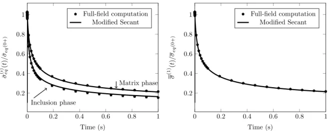
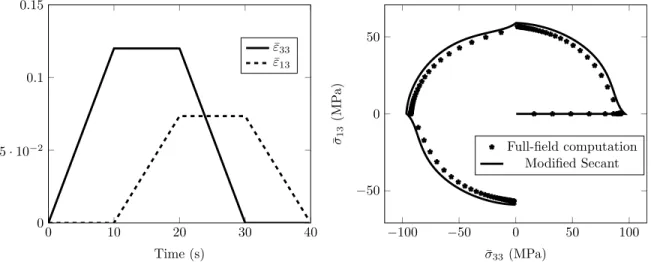
In view of this, the present work uses the nonlinear variational homogenization method (Ponte Casta˜ neda [29]) or equivalently the modified secant method (Suquet [43]), which makes

It has been shown that the use of the macroscopic strain and stress as references in the context of the ‘second- order’ homogenization method leads to simple and accurate estimates

The present study introduces a methodology that allows to combine 3D printing, experimental testing, numerical and analytical modeling to create random closed-cell porous materials

Adopting a stress-based approach, we have extended the classical variational principle of Hashin and Shtrikman (1962a) to stress-gradient materials, first for periodic