A three-dimensional synthesis study of δ 18 O in atmospheric CO 2 : 1. Surface fluxes

HAL Id: hal-02923804

https://hal.archives-ouvertes.fr/hal-02923804

Submitted on 28 Oct 2020

HAL is a multi-disciplinary open access

archive for the deposit and dissemination of

sci-entific research documents, whether they are

pub-lished or not. The documents may come from

teaching and research institutions in France or

abroad, or from public or private research centers.

L’archive ouverte pluridisciplinaire HAL, est

destinée au dépôt et à la diffusion de documents

scientifiques de niveau recherche, publiés ou non,

émanant des établissements d’enseignement et de

recherche français ou étrangers, des laboratoires

publics ou privés.

A three-dimensional synthesis study of δ 18 O in

atmospheric CO 2 : 1. Surface fluxes

Philippe Ciais, A. Scott Denning, Pieter Tans, Joseph Berry, David Randall,

G. James Collatz, Piers Sellers, James White, Michael Trolier, Harro Meijer,

et al.

To cite this version:

Philippe Ciais, A. Scott Denning, Pieter Tans, Joseph Berry, David Randall, et al..

A

three-dimensional synthesis study of δ 18 O in atmospheric CO 2 : 1.

Surface fluxes.

Journal of

Geophysical Research: Atmospheres, American Geophysical Union, 1997, 102 (D5), pp.5857-5872.

�10.1029/96JD02360�. �hal-02923804�

JOURNAL OF GEOPHYSICAL RESEARCH, VOL. 102, NO. D5, PAGES 5857-5872, MARCH 20, 1997

A three-dimensional

synthesis

study

of

in atmospheric

COz

1.

Surface fluxes

Philippe Ciais,

• A. Scott Denning,

2 Pieter P. Tans,

3 Joseph A. Berry,

4

David A. Randall, 2 G. James Collatz, s Piers J. Sellers, s James W. C. White, 6

Michael Trolier, 3,6 Harro A. J. Meijer, 7 Roger J. Francey,

s

Patrick Monfray, 9 and Martin Heimann •ø

Abstract. The isotope

•SO

in CO2 is of particular

interest

in studying

the global

carbon

cycle because it is sensitive to the processes by which the global land biosphere absorbs

and respires CO2. Carbon dioxide and water exchange isotopically both in leaves and in

soils,

and the •SO character

of atmospheric

CO2 is strongly

influenced

by the land biota,

which should constrain the gross primary productivity and total respiration of land

ecosystems.

In this study

we calculate

the global

surface

fluxes

of •SO for vegetation

and

soils using the SiB2 biosphere model coupled with the Colorado State University general

circulation model. This approach makes it possible to use physiological variables that are

consistently weighted by the carbon assimilation rate and integrated through the

exchange of O and the isotopic

vegetation

canopy.

We also

calculate

the air-sea

rs

character of fossil emissions and biomass burning. Global mean values of the isotopic

exchange

with each

reservoir

are used

to close

the global

budget

of •SO

in CO2.

Our

results confirm the fact that the land biota exert a dominant control on the (5•SO of the

atmospheric reservoir. At the global scale, exchange with the canopy produces an isotopic

enrichment of CO2, whereas exchange with soils has the opposite effect.

1. Introduction

Increasing attention has been given recently to the terrestrial biosphere in controlling atmospheric CO2 levels because the carbon stored in the aboveground biomass and in soil organic matter can be exchanged rapidly with the atmosphere. It is well recognized that land ecosystems take up and release large quantities of CO2 not only on a daily and seasonal timescale but also in the long term. Several models of the global bio- sphere on land have been developed which simulate the be-

havior of various ecosystems and have been used in order to

predict the carbon fluxes exchanged with the atmosphere un- der specific scenarios of future climate change including ele-

•Laboratoire de Mod61isation du Climat et de l'Environnement,

Commissariat h l'Energie Atomique l'Orme des Merisiers, Gif sur Yvette, France.

2Department of Atmospheric Sciences, Colorado State University,

Fort Collins.

3Climate Monitoring and Diagnostic Laboratory, NOAA, Boulder,

Colorado.

4Department of Plant Biology, Carnegie Institution of Washington, Stanford, California.

SNASA Goddard Space Flight Center, Greenbelt, Maryland. 6Institute of Arctic and Alpine Research and Department of Geo-

logical Sciences, University of Colorado, Boulder.

7Centrum voor Isotopen Onderzoek, University of Groningen, Gro-

ningen, Netherlands.

8Division of Atmospheric Research, Commonwealth Scientific and

Industrial Research Organisation, Melbourne, Victoria, Australia.

9Centre des Faibles Radioactivit6s, Laboratoire de Mod61isation du

Climat et de l'Environnement, Gif sur Yvette, France.

•øMax-Planck-Institut ffir Meteorologie, Hamburg, Germany.

Copyright 1997 by the American Geophysical Union. Paper number 96JD02360.

0148-0227/97/96JD-02360509.00

vated atmospheric CO2 levels, changing nutrient availability, temperature, and precipitation patterns.

Models of ecosystem functioning have become progressively more process oriented, especially regarding the photosynthetic uptake of CO2. A few global mechanistic models based on external "climatic" forcing, such as the incident solar flux, the water availability for plants, and the temperature, are able to calculate the gross fluxes of CO2 exchanged between land ecosystems and the atmosphere. Figure la gives a schematic picture of the cycling of carbon between plants, soils, and the atmosphere. Of particular importance to the atmospheric CO2 budget is the uptake of CO2 by photosynthesis (A is gross

primary productivity (GPP) minus leaf respiration •d) and the

accompanying ecosystem total respiration (•). Respiratory

CO2 emissions include aboveground plant respiration ^

(•plants)

and belowground root respiration B

trophic soil respiration (•soi•s), the total CO2 effiux from soils

being called Fsoil s. Over the course of the year, the annual mean assimilation A is almost entirely compensated by respi- ration emissions.

The CO2 biospheric fluxes calculated by ecosystem models can be partially validated against atmospheric observations. For instance, a very useful validation is to compare the sea- sonal variation in atmospheric CO2 simulated with given bio- spheric fluxes to the well-documented observational record at numerous sites around the world [Conway et al., 1994]. This is commonly done by coupling the calculated field of the net ecosystem flux of CO2, the difference between A and •, to an atmospheric transport model, and comparing the results to observations. This approach has proven very valuable for test- ing the seasonality of net CO2 fluxes [e.g., Fung et al., 1987] but does not constrain the gross fluxes of CO2 separately.

The global budget of atmospheric CO2 has also been studied

using measurements of the /5•3C of atmospheric CO2. The

5858 CIAIS ET AL.: STUDY OF &•80 IN ATMOSPHERIC CO2, 1

FAL ingoing

CO2

FLA retrodiffusion

of

CO2

A

•Plants

Fso,s

•

stem, twigs '•' total soil • total

respiration respiration respiration

•lant

!plant below- soil heterotrophic

:ground respiration respiration

Figure la. (a) The cycling of carbon between the land biosphere and the atmosphere. The ecosystem represented is in equilibrium since the annual mean uptake of CO2 by photosynthesis (A) compensates exactly the total respiratory loss (•).

method

relies

on the interpretation

of atmospheric

8•3C

vari-

ations as indicating net biospheric fluxes [Tans et al., 1993; Francey et al., 1995; Keeling et al., 1995;Enting et al., 1993, 1995; Ciais et al., 1995]. The method is limited by uncertainty con- cerning the influence of isotopic disequilibria between atmo- sphere and surface reservoirs. Such disequilibria can be trans- ferred to the atmosphere by gross exchange fluxes, even in the absence of net exchange.

The Earth's vegetation likely exerts a major influence on the

•80/•60 ratio of atmospheric

CO2 [Keeling,

1995].

Francey

and

Tans [1987] first pointed out that the isotopic exchange with water in leaves (and possibly soils) may determine the ob-

served persistent north-south differences in 1gO of atmospheric

CO2. Farquhar et al. [1993] further quantified the global role of leaf exchange and calculated a global atmospheric budget of

180 in CO2.

Specifically,

the lgo/•60 ratio of atmospheric

CO:

is controlled by the fluxes A and •. We present here a syn-

thesis simulation of •gO in CO2 that we compare with atmo-

spheric measurements. In the present paper we focus on the

mechanisms that govern the •gO/•60 ratio in CO:. Specifically,

we have calculated on a 4 ø by 5 ø grid the isotopic fluxes asso-

ciated with the terrestrial and oceanic reservoirs, as well as

with anthropogenic CO: emissions. In the companion paper by Ciais et al. [this issue] we have prescribed these fluxes in the three-dimensional atmospheric tracer model TM2 and com-

pared

the simulated

8•80 values

to atmospheric

observations.

1.1. Conventions and Units

In this paper, sinks correspond to a negative net flux of carbon (CO2 is removed from the atmosphere) and sources correspond to a positive net flux (CO2 is released to the atmo- sphere). Isotopic ratios are expressed in per mil (%0), defined as

8180 = 1000

18

16 180/160

( O/ O)sampl e -- ( )standard

18t•/16t•\ •J/ •JJstandard

For CO> all isotopic values are given relative to the stan- dard isotopic ratio Vienna Pee Dee belemnite (VPDB)-CO: = 0.002088349077 as recommended by Allison et al. [1995]. For H:O we express isotopic abundance relative to the standard Vienna SMOW (VSMOW) = 0.00200520 [Baertchi and Mack- fin, 1965]. We must subtract 41.47%o to express VSMOW values in the VPDB-CO: scale. This includes a difference of

-30.9%0 between VSMOW and VPDB-calcite [Hut, 1987]

and accounts for the •gO fractionation during CO: evolution at

25øC with 100% phosphoric acid [Friedman and O'Neill, 1977] between VPDB-calcite and VPDB-CO2.

1.2. Climate Variables Used in This Study:

CSU GCM and SiB2 Model

The Colorado State University (CSU) general circulation model (GCM) is derived from the University of California, Los Angeles, (UCLA) GCM, which was developed at UCLA over a period of 20 years by A. Arakawa and collaborators. A copy of the model was brought to the Goddard Laboratory for Atmospheres in 1982 and from there to CSU in 1988. Many changes have been made since the model left UCLA, including revised parameterizations of solar and terrestrial radiation [Harshvardhan et al., 1987], the planetary boundary layer (PBL) [Randall et al., 1992], cumulus convection [Randall and Pan, 1993], cloud microphysical processes [Fowler et al., 1995], and land-surface processes [Sellers et al., 1986, 1992a, b, 1996a, b]. Some recent results are presented by Randall et al. [1989, 1991, 1996], Fowler et al. [1995], and Fowler and Randall [1995a, b].

The prognostic variables of the CSU GCM are potential temperature; the horizontal wind components; the surface pressure; the PBL's depth and turbulence kinetic energy; the mixing ratio of three phases of water plus rain and snow; the temperatures of the plant canopy, the ground surface, and the deep soil; the water contents of four aboveground and three

CIAIS ET AL.: STUDY OF 8•80 IN ATMOSPHERIC CO2, 1 5859

belowground moisture stores; the stomatal conductance of the plant canopy; and the ice temperature at land ice and sea ice points. The governing equations are finite-differenced, using highly conservative schemes [Arakawa and Lamb, 1977, 1981]. The model is formulated in terms of a modified sigma coordi- nate, in which the PBL top is a coordinate surface, and the PBL itself is identified with the lowest model layer [Suarez et al., 1983]. The mass sources and sinks for the PBL consist of large-scale convergence or divergence, turbulent entrainment, and the cumulus mass flux. Turbulent entrainment can be driven by positive buoyancy fluxes or by shear of the mean wind in the surface layer or at the PBL top.

For vegetated land points the surface fluxes of sensible and

latent heat, radiation, moisture, and momentum are deter-

mined using the simple biosphere (SiB) parameterization de- veloped by Sellers et al. [1986]. SiB has recently undergone substantial modification [Sellers et al., 1996a, b; Randall et al., 1996] and is now referred to as SiB2. The number of biome- specific parameters has been reduced, and most are now de- rived directly from processed satellite data rather than pre- scribed from the literature. The vegetation canopy has been reduced to a single layer. Another major change is in the parameterization of stomatal and canopy conductance [Collatz et al., 1991, 1992; Sellers et al., 1992a, b, 1996a] used in the calculation of the surface energy budget over land. This pa- rameterization involves the direct calculation of the rate of carbon assimilation by photosynthesis, making possible the calculation of CO2 exchange between the atmosphere and the terrestrial biota at the dynamic time step (6 min) of the CSU GCM [Denning, 1994; Denning et al., 1996; Denny and Randall, 1996]. Details of the carbon flux calculations and their use in isotopic exchange calculations are presented in Appendix B.

2. Oxygen Isotope Fractionation Between COz

and HzO

Of major importance for the isotopic composition of CO2 in the atmosphere is the fact that dissolved CO2 may exchange an

•80 atom with water according to the isotopic equilibrium

reaction (1):

COO + H2180

<-• CO•80 + H20

(1)

where

O stands

for •60, the dominant

oxygen

isotope.

When reaction (1) occurs in nature, there is more water than

CO2 by several orders of magnitude. This implies that •80 of

CO2 is entirely determined by •80 of the reacting water,

whereas •80 of water is negligibly altered by the reaction. For

CO2 isotopically equilibrated with water according to reaction

(1), the equilibration

factor

Oteq

is defined

as

•80/•60 ratio of CO2 after equilibration

O/eq

(T) =

180/160

ratio

of

reacting

H20

(2)

We use

the value

of Oteq

(T) determined

by Brenninkmeier

et al.

[1983].

( •eq

)

O/eq

(T) = 1 + 1000

eeq --- 17604/T - 17.93

At 25øC,

eeq

: +41.11%o

and

deeq/dT

= -0.20%0 øC

-•.

Direct isotopic exchange between CO 2 and H20 vapor is excluded because the rate of hydration is slow (several min- utes) and only a very small fraction of CO2 is dissolved in liquid water at any time [Francey and Tans, 1987]. However, the enzyme carbonic anhydrase (CA), ubiquitous in plant tissues, catalyzes the hydration and strongly accelerates the rate of reaction (1) [Silverman, 1982]. In living plant tissues the isoto- pic equilibrium between CO2 and H20 is reached quasi- instantaneously. Little is known of CA activity in soils, but CO2 produced from decaying plant tissues remains in contact with soil water for sufficient time (see below) for reaction (1) to occur and most likely yield full isotopic equilibration of CO2

with water, even in the absence

of CA. The •80 of CO2 in

leaves and in soils can therefore be predicted by reaction (1),

provided

we know

the •80 of water

reacting

with CO2 and the

temperature of reaction.

One difficulty is to clearly identify the isotopic composition of water that exchanges isotopically with CO2. Thus it is im- portant to characterize precisely in which leaf organ and in which soil compartment the isotopic reaction of CO2 with water occurs [e.g., Yakir et al., 1994]. Generally, such informa- tion is not directly available from experiments, and we have to make a few arbitrary but reasonable assumptions in order to

calculate

the surface

fluxes

of •80 in CO2.

In the following,

we

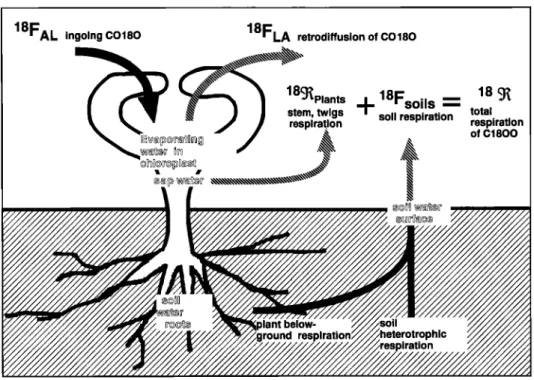
detail the parameterization of the isotopic exchange with the biospheric and oceanic reservoirs and the isotopic character of CO2 derived from fossil fuel burning. The CO2 oxygen isotope fluxes with the land biota are shown in Figure lb.

3. Isotopic Exchange in Soils

Processes which oxidize carbon in soils usually cause CO2 levels to be greater in the soil than in the atmosphere, by up to several thousands of parts per million [D6rr and Munnich, 1987]. A complication arises because root respiration and the decomposition of dead organic matter by microorganisms emit CO2 at various depths. However, even without catalysis of the reaction (1) by the enzyme CA, CO 2 would diffuse upward

slowly enough to fully exchange •80 with water in the soil.

From the diffusivity (D) of CO2 in soils, D = Keo(1 - [3) D a [Hesterberg and Siegenthaler, 1991], with G 0 the dry po- rosity (0.5), (1 - /3) the air-filled pore fraction of the soil (0.20), K the tortuosity (0.66), and D a the diffusivity of CO2 in

air (0.15 cm

2 s-•), we estimate

that the average

time taken

by

a CO2 molecule emitted at x = 30 cm depth to reach the

atmosphere

is 6 hours

(t = x2/4D) (the tortuosity

accounts

for

the fact that the shortest path of CO2 can be blocked by soil particles). This is much longer than the time necessary for the hydration of CO 2 in the soil pores • koeofl which is approx- imately 7 min, given k0 the rate of hydration in bulk water at

10øC

(6.9 10

-3 S-•). This holds

if the Bunsen

(volumetric)

solubility coefficient is close to 1, which is true for CO2. Prac- tically, this means that CO2 equilibrates with water within the top 4 cm of soils, whatever its original isotopic composition at depth. In the presence of active CA in soil organic matter the isotopic exchange would be even much faster.

Thus we calculate •80 of CO2 in soils from surface ground

temperature

and from •80 of water at the soil surface,

which

is derived from meteoric water [Jouzel et al., 1987]. Conse-

quently,

•80 of CO2 respired

by soils

is expected

to follow

the

seasonal changes in the isotopic composition of precipitation

and in temperature. The respired flux of species CO•80 is

586O CIAIS ET AL.: STUDY OF 8180 IN ATMOSPHERIC CO22 1

18FAL

ingoing

CO180

18FLA

retrodiffusion

of

CO180

18•Plant

s

18 •

stem,

•,.s

+ 8Fsøi's

soil

respiration

=

total

respiration respiration

_"•

_A

_of

_C1800

Figure lb. The pertainent

180 exchange

fluxes.

Atmospheric

CO2 entering

the leaves

reacts

isotopically

18Fsoll S = O•sRsFsoll S (3)

Fsoii s is the flux of CO2 emitted by soils (sum of plant below- ground respiration and soil heterotrophic respiration as in

Figure

lb); Rs is 180/160

ratio of CO2 equilibrated

with sur-

180 during diffusion between the soil surface and the atmo-

sphere. We infer es = -5%0 from the global budget of atmo-

spheric

8180 (see

section

7).

3.1. CO2 Exchange Fluxes

It is important to note that the flux of CO2 respired below- ground, Fsoii s, includes both root respiration and heterotrophic

respiration.

Whatever

the 8'80 of CO2 produced

at depth,

its

at the surface of the soil. Additionally, a small fraction of the

plant respiration flux is emitted aboveground by stems and

twigs. We assume that CO2 in stems is in isotopic equilibrium

with water and that stem water 8•80 is identical to groundwa-

ter 8180 because of negligible fractionation during the uptake of water by roots and the ascent of sap. The fact that there is

almost no difference between 8•80 of groundwater and of

water in the plants organs, leaves excepted, has been clearly

demonstrated by Bariac et al. [1994a, b]. Consequently, we can

treat the isotopic exchange of CO2 respired by stems in the

same manner as CO2 respired belowground, which means that

Fsoi• s in (3) must be augmented by the stem respiration flux. In other words, we replace Fsoi• s by the total respiration flux ffl

defined in Figure la.

3.2. The •80 of Water in Soils

Assuming isotopic equilibrium of CO2 with water at the soil

surface, we have

R s : O/eq (rs) Rs w (4)

where R7 is 180/160 ratio of surface groundwater and T s is

surface ground temperature.

In (4) we use the temperature fields predicted by the GCM. The isotopic composition of surface groundwater R7 is very

close to that of meteoric water, which we take from the God-

dard Institute for Space Studies (GISS) GCM [Jouzel et al., 1987] (see Appendix A for details). Alternatively, we could

have

used

a global

regression

of the available

data

for 8180 of

GISS simulation for consistency because our modeling of can-

opy processes (section 4) also requires the use of the field of 8•80 in water vapor as calculated by the GISS model, for which

there

is no global

data set.

The annual

mean

8•80 in meteoric

water calculated by Jouzel et al. [1987] is nevertheless in satis-

factory agreement with the data of the IAEA global network

[IAEA, 1981]. However, over South America and Africa, the

GISS GCM may underestimate 8•80 in precipitation by 2-3%0

[Jouzel et al., 1987].

Plate la shows the annual mean 8•80 in surface groundwa-

ter, R7. This variable,

following

8•80 in meteoric

water, de-

tion from air masses initially formed over the ocean and ad- vected inland. Owing to large-scale circulation patterns and to

temperature,

the lowest

values

of 8180

in surface

groundwater

occur over inland North America and over Siberia, with an

average decrease of -14%o between the equator and the arctic

(ice sheets excepted).

Plate lb shows the isotopic composition of CO2 in the soil

surface layer (i.e., CO2 exchanged between the surface ground- water and the atmosphere). Common features with the map of

8180

in surface

groundwater

include

depletion

of 180 at high

CIAIS ET AL.' STUDY OF 8•80 IN ATMOSPHERIC CO2, 1 5861

O/eq

in (4) opposes

the latitudinal

profile

of 8180

in groundwa-

ter: colder temperatures at high latitudes increase the value of

O•eq

(i.e., produce

an isotopic

enrichment

of CO2). As a result,

the 8180 difference

in soil CO2 between

the tropics

and the

high northern latitudes is only of -7%0 (Plate lb), compared

to -14%o for 8•80 in soil water.

4. Isotopic Conversion in Leaves

Tans et al. [1986] first suggested that the isotopic exchange of

CO2 and water in leaves may exert a large control on 8180 in

atmospheric CO2 to explain the observed isotopic depletion of the atmosphere at high northern latitudes. The role of leaves was further quantified by extending the physiological proper- ties of different kinds of plants to global ecosystems [Farquhar et al., 1993]. These interpretations rely on the assumption that CO2 equilibrates instantly with water in leaves because CA is ubiquitous. The presence of CA guarantees fast isotopic equi- librium, whereas without CA, CO2 diffusing from the meso- phyll cell would not reach full equilibrium. Given Dw the dif-

fusivity of CO2 in water (1.5 10 -s cm -2 s -1 at 10øC), the average time to cross a distance x = 10 -s m within the

mesophyll cell (from the site of carboxylation to the stomatal

cavity)

is roughly

0.02 s (t = x2/4Dw),

much

less

than the time

required for hydration of CO2 in bulk water, approximately 3 min at 10øC. Note also that only isotopic exchange with water inside the leaf is considered and that we do not treat the exchange with dew or with water intercepted by the canopy.

Interactions with leaf water involve an even larger flux of CO2 than the gross photosynthetic rate of carbon assimilation. All of the atmospheric CO2 which enters the leaf undergoes hydration and isotopic equilibration with water, but less than half of that CO2 is fixed, with the remainder returning to the

atmosphere.

The exchange

of CO180 is therefore

fundamen-

tally different from other CO2 exchange. Only the net ecosys- tem flux of CO2 is needed for the simulation of CO2 concen-

trations

and 13C/12C

isotope

ratios

in the atmosphere.

With

respect

to 8180 in atmospheric

CO2, however,

the gross

leaf

exchange is very important because retrodiffused CO2 carries an isotopic label distinct from CO2 going into the leaf (Figure

lb). The net flux of C18OO

which

interacts

with the •80 res-

ervoir of leaf water is given by

18EL ... -- --OtdRaFaL + O/dRLFLa (s)

The equivalent net flux of CO2 is

A = --FaL q- FLa (6) where

A assimilation rate of carbon (<0);

RE 180/160

ratio of CO2 in isotopic

equilibrium

with leaf

water;

R a 180/160

ratio of CO2 in the atmosphere

at the leaf

surface;

Fat" mean flux of CO2 entering the leaf (CO2 which crosses the stomate and further diffuses to the chloroplast but without being reduced by photosynthesis), defined as a positive quantity; Fna mean flux of retrodiffused CO2 (CO2 which diffuses

back to the atmosphere), defined as a positive quantity;

ot d kinetic fractionation of C18OO for diffusion in air,

identical to 1 + (ed/1000) (8 d : --8.8%0).

Equation (5) can be rewritten as

18FL

... --' ozdgaA

- OtdFLa(g

a --RL)

(7)

Equation (7) formally separates the isotopic exchange of CO2 between leaves and atmosphere into two terms. The left- hand member represents the isotopic fractionation associated with the net flux into the leaves. It represents CO2 that is almost matched isotopically with the atmospheric value (pro- portional to Ra), thus having a very limited influence on it. The right-hand member is an "isotopic disequilibrium flux," pro-

portional to the 180/160 difference in CO2 between the leaves

and the atmosphere and therefore exerting a strong control on the atmospheric signature. In the following, we detail the ex- pression of each variable in (7), starting with the CO2 exchange fluxes represented in Figure la.

4.1. CO2 Exchange Fluxes

The gross assimilation rate of CO2 (A) is given by A = -gs(Ca- Cc) (8) where C c is CO2 concentration inside the leaf, Ca is CO2 concentration in the air outside the leaf, and g• is stomatal conductance.

The flux A is the net assimilation of carbon, in other words,

the amount of CO2 that is reduced by photosynthesis and stored into plant assimilates. A is the difference between the

GPP and the leaf respiration (•d). Thus leaf respiration is part

of the retrodiffused flux FLa. Globally, •d consumes about

12% of annual GPP in the model, so A = 88% of GPP. Also,

we treat the full diffusive path of CO2 from outside the leaf to the site of carboxylation using one single conductance, g•, here called "stomatal conductance" which accounts in fact for the diffusion of CO2 through the leaf aerodynamic boundary layer,

the stomate, and the recess of stomatal cavities. We use fields

of A and Cc calculated by SiB2, as detailed in Appendix B [Sellers et al., 1996a; Randall et al., 1996; Denning et al., 1996]. The one-way gross fluxes Fna and Fau of (7) are expressed by FaL-' gsCa FLa = gsCc (9) Substituting for #s from (8) into (9) yields

FaL

= -- (C

•

a __

Cc

A

FLa

= -- (C

a _ Cc

) A

(10)

A global estimate of fluxes in (7) is possible since it is commonly observed that Cc = 2/3 Ca for C3 plants (see Table 1), which yields Fan • 3A and Fna = 2A. We find that FaL

and Fna, equal 22.7 and 14.2 Pmol yr- 1, respectively, with A =

8.5 Pmol yr -1 from SiB2. The fluxes Fan and Fna of CO2 are

enormous. They imply that every molecule of CO2 in the at- mosphere has only a 14% chance to be actually assimilated by photosynthesis against a 40% chance to enter a leaf within a

year!

The flux calculations presented here were conducted off-line using monthly mean fields of parameter values calculated by SiB2, as detailed in Appendix B [Sellers et al., 1996a; Randall et al., 1996; Denning et al., 1996]. The carbon and water budget of the land surface is calculated explicitly and interactively by the SiB2 model coupled to the CSU GCM. This approach has the advantage that monthly means reflect well-resolved diurnal cycles of the relevant variables in a dynamically consistent way. The disadvantage is that one has to rely on the climate simu-

5862 CiAIS ET AL.: STUDY OF 8180 IN ATMOSPHERIC CO2, 1

Table 1. Notations and Principal Fractionations, Diagnostics, and Physiological Variables That Enter in the 8•80 Sources

CO2 Fluxes* Description Global Mean Unit of Measure

FaI. atmospheric CO2 entering the leaf 22.7 Pmol CO2 Fi.a CO2 retrodiffused out of the leaf 14.2 Pmol CO2 Fsoil s CO 2 effiux from soils, augmented by stems and twigs 8.5 Pmol CO2 .4 respiration (equals total respiration) net carbon assimilation 8.5 Pmol CO2

rate (gross primary productivity minus leaf respiration)

Foa gross CO2 transfer from ocean to atmosphere 7.5 Pmol CO2

Fao gross CO2 transfer from atmosphere to ocean 7.7 Pmol CO2

Fo net air-sea flux of CO2 167 Tmol CO2

Ff fossil CO2 emissions 500 Tmol CO2

Fbu r biomass burning CO2 emissions 283 Tmol CO2

Physical and

Physiological Variables Description Global Mean Unit of Measure

h leaf surface relative humidity 0.8

Ti. leaf temperature 12.1

T s ground surface temperature 12.0 T O sea surface temperature 17.9 C i CO 2 mixing ratio inside leaf

average for C3 plants only average for C4 plants only average for both C3 and C4

220 113 195 o C o C o C ppm ppm ppm Atmospheric 8180 and

CO2 Mixing Ratios Description

•a, C a 8i., Ci.

8ø, C O 8b, Cb 8f, Cf

8•80, CO2 in the atmosphere

8•80, CO2 resulting from leaf exchange 8•80, CO2 resulting from soil exchange 8•80, CO2 resulting from ocean exchange 8180, CO2 resulting from biomass burning 8180, CO2 resulting from fossil fuel emissions

Fractionation Factors e = (a -1)10 -3,

of Oxygen Isotope Description %o Comments

O/eq fractionation of CO180 in the isotopic reaction with water +41.15

% fractionation of CO180 during diffusion from the soil -5

surface to the atmosphere

ad fractionation of CO•80 during diffusion between the -8.8 Molecular diffusion

chloroplast and the atmosphere

fractionation of CO•80 during diffusion and hydration in

water

fractionation of H2•80 with respect to the liquid phase

during the Liquid -• vapor phase transition

fractionation of H2180 during the diffusion of water vapor

from inside the leaf to the air

discrimination of •80 by leaf exchange

aw +0.8 w O/L--vap w o/k +9.39 -26.3 A a 7.22 Equilibrium value at 25øC Molecular and turbulent diffusion

Equilibrium value at 25øC

Molecular and turbulent diffusion

Global average value weighted by

monthly GPP (.4) Isotopic Ratios? Description Global Mean, %o Comments

Ra atmospheric CO2 0.18

R• CO2 in isotopic equilibrium with surface groundwater -5.15 R t_ CO2 in isotopic equilibrium with leaf water 3.27 Ro CO2 in isotopic equilibrium with ocean surface water + 1.75 R f CO2 produced by combustion with atmospheric 02 -17 R w P meteoric water over continents -7.88

R•' surface groundwater -7.55

R, w intermediate (root zone) groundwater -7.55

R• evaporating water in leaves 0.40

R w _{vap water vapor in the canopy -17.9}

Rj ocean surface water 0.26

PDB-CO2 scale

VSMOW scale

*The same notations with an exponent 18 are used for the CO•80 surface fluxes.

?The same subscripts are used for 8.

Some of the calculations in this study required special aver- aging to avoid errors due to nonlinear interactions. For exam- ple, because C c covaries withA, the calculated monthly sum of FLa (equation (10)) would be expected to be very different if

evaluated as the sum of every time step for a month, or if evaluated using the mean monthly values of Cc, Ca, andA for that month. In other words, the mean of the product of terms is not equal to the product of the means of those terms. The

CIAIS ET AL.' STUDY OF 8180 IN ATMOSPHERIC CO2, 1 5863

a)

(•180 in Surface Ground Water

%o V-SMOW

Global Mean = -7.6

30

,• . ., .

¾,•,.-

, ,,,•. - , , ,"

! I i,21

'

b)

(•180

in CO

2 at the Soil

Surface

NP

%o V-PDB-CO2

Global Mean = -4.7

-'7 '"-• •.. '--.•.

o /

}

. •

...

ß

-30

••.•

• '

Plate 1. (a) Surface

groundwater

annual

mean

8•80 determined

from the isotopic

composition

of meteoric

water in the NASA GISS isotopic GCM, after Jouzel et al. [1987] and Appendix A. (b) Annual mean isotopic

composition of CO2 at the soil surface assuming full isotopic equilibrium with surface groundwater. The •80

of CO2 in soils,

mediated

by the respiration

effiux,

directly

influences

the atmospheric

•80.

5864 CIAIS ET AL.: STUDY OF 8•80 IN ATMOSPHERIC CO2, 1

correct answer can be calculated on-line, or off-line by using an average value of C c weighted for the value of A in each time step. We did the latter. The product A by C c was calculated at each time step of the GCM run (excluding times when A was negative). This product was summed for the averaging period and divided by the sum of A for that period, yielding a flux- weighted average. Canopy temperature was similarly weighted for physiological activity. We are aware of additional possibil- ities for nonlinear averaging errors in the use of mean monthly GCM fields for calculation of isotopic fluxes (for example, the time average humidity at the leaf surface was used, and we recognize that this should ideally be weighted for the rate of CO2 exchange). It would obviously be best to include all of these calculations explicitly in the model. This will be done in a future study.

4.2. The •i•80 in Leaf CO2

We calculate the 180/160 ratio of leaf CO2, RL, based on R•

the isotopic composition of evaporating leaf water (see below), assuming that CO2 reaches full isotopic equilibration with wa- ter evaporating in the mesophyll cells at leaf temperature TL [Farquhar et al., 1993]:

g L : O/eq(rL)g • (11)

A recent set of experiments by Yakir et al. [1994] suggests that CO2 may not in reality exchange isotopically with evaporating water but with a pool of leaf water which is at an intermediate isotopic state between evaporating water at {5• and water sup-

plied to the leaf by roots at {5•'. If this is confirmed, we would

then infer leaf CO2 to be too enriched by following Farquhar et al. [1993].

Evaporating

water in leaves

is enriched

in 180. At steady

state, and for a constant leaf water volume, the evaporating

leaf water 180/160

ratio R• is given

by [Craig

and Gordon,

1965]

= w

R• OtL_va

p

+ hRv'•p

)

(12)

Using the {5 notation, (12) can also be written as

{5• '- 8•-vap

q- (1 -- h)({5/w

- 8•) q- h{sv•

p

h relative humidity at the leaf surface;

a w

fractionation

of H2•80 for the liquid-vapor

phase

transition,

equal

to 1 + (•_vap/1000)

----

R•/RvWap;

diffusion of water vapor across the stomatal cavity and leaf boundary layer, equal to 1 + (•'/1000);

Rv•

p 180/160

ratio

of water

vapor

in the air outside

the

leaf;

R•' •80/160 ratio of groundwater

which

is taken

up by

roots.

The first important

parameter

in (12') is {5•',

the {5180

of

groundwater delivered to the leaf. At steady state an equiva- lent amount of water delivered to the leaf and lost by transpi- ration must be pumped from the soil by the root system. Fol- lowing the hypothesis of the SiB2 model soil hydrology, we consider that the roots pump groundwater from an intermedi- ate soil layer beneath the surface (Figure A1 in Appendix A). Assuming that no isotopic fractionation occurs during the root uptake of water [Bariac et al., 1994b], we calculate {5•" from the

{5180 of meteoric water and from the soil water fluxes in SiB2

through a mass balance of groundwater isotopes as described in Appendix A.

A second important parameter in (12') is the kinetic frac- tionation of water vapor in leaves •', which bears a large uncertainty. The value of •' is greater for molecular diffusion (-28.5%0) [Merlivat, 1978] than for turbulent diffusion and may thus be species specific [White, 1983] and depend on the wind velocity [F6rstel et al., 1975]. However, this source of uncertainty is diminished by the fact that •' is multiplied by a factor of ( 1 - h) which takes on low values almost everywhere (Plate 2a). The only exceptions correspond to dry areas, but these regions are usually associated with very small CO2 fluxes (negligible GPP). We have taken •' = -26.3%0 [Farquhar et al., 1989] constant everywhere. A detailed study of the sensi-

tivity of {5180 in atmospheric CO2 to •' will be presented

elsewhere.

The third important

parameter

in (12) is {5180

in the canopy

water vapor. Because there are only sparse measurements of this quantity around the world, we use the GISS GCM simu- lation at ground level as plotted in Plate 2b. As pointed out in

section

3.2, consistency

dictates

that we also

use {5180

of sur-

face groundwater (close to meteoric water) from the same model since the difference between these fields enters in (12'). The condensation processes which form the precipitation in clouds follow an isotopic fractionation which systematically

depletes

180 in the vapor

with respect

to the precipitation.

On

average,

{5180

in water vapor

is lower than {5180

in meteoric

water by about 10%o. One large source of uncertainty is that

the {5180

of the vapor

in open

air from the GISS GCM may

not

be representative of the situation in forest canopies. This

source

of uncertainty

is augmented

in (12') by the fact {5180

of

water vapor is multiplied by the relative humidity at the leaf surface, which is generally close to unity within the leaf bound- ary layer (Plate 2a). In canopies, substantial quantities of water vapor are derived from plant transpiration with an isotopic label identical to groundwater (10%o above the tropospheric vapor value). To the extent that water in the canopy air space

reflects

this source,

the {5180

in water

vapor

inferred

from the

GISS model is probably too low. From isotopic measurements in water vapor over a grassland in Switzerland, Jacob and Sonntag [1991] suggest that the share of vapor released by plants varies between 15% in winter and 80% in July- September. Measurements in a temperate forest by White and Gedzelman [1984] suggest that the relative humidity can be

used

to distinguish

between

free tropospheric

vapor

({5180

-->

w

{sv•p

•tm)

in the

limit

h -->

0 and

plant

transpired

vapor

({5180

-->

regression to the global level to correct {5180 of vapor in can-

opy, however. By using the GISS model fields we instead as-

sume

a lower

boundary

for {5180

in water

vapor

and hence

for

{5•80

of CO2 in leaves.

Plate 2c shows {5•80 of leaf CO2, which decreases toward

high

latitudes.

Over dry areas,

{5180

of leaf CO2 is larger

than

6%0, with a maximum over the Sahara Desert of 15%o. This is

mostly due to low relative humidity which increases the value of {SL in (12). Note, however, that the maximum values ob-

tained

in deserts

is not likely

to influence

the atmospheric

{5180

because it is associated with a negligible exchange of CO2. The simulated isotopic composition of leaf CO2 is as low in tropical rainforests as in Siberian forests (roughly -3%o), despite the

a)

Relative Humidity at the Leaf Surface

Percent

Global Mean-

79.2

NP ß ß :. ß - ; .... ?,., ½, 3O EQ -30 -60 8P 180 120 W 60 W 0 60 E 120 E 180 15.0 25.0 35.0 45.0 55.0 65.0 75.0 85.0 95.0 10.0 20.0 30.0 40.0 50.0 60.0 70.0 80.0 90.0

b)

•180 in Water Vapor

at Ground

Level

%0 V-SMOW

Global Mean-17.0

NP

c)

•180 of CO

2 in Leaves

%0 PDB-CO2

Global Mean-

3.2

NP .. . .• ,,, .. •.,, ... ..?.. ... .,,* •,•

30

e

",.•...•:.:,.,•-::-'.•

\ '-- ':'

'

Plate 2. (a) Relative humidity at the leaf surface (annual average) in the photosynthesis model SiB2 coupled

with the CSU climate model. Because of plant transpiration the relative humidity at the leaf surface is higher

than

in the free atmosphere

above

the canopy.

(b) Annual

mean

•80 of atmospheric

water

vapor

at ground

processes.

(c) Annual

mean

t5•80

of CO2 in leaves,

that is, in isotopic

equilibrium

equilibrated

with evapo-

rating

leaf water.

This corresponds

to the t5•80

which

influences

the atmosphere,

mediated

by the photosyn-

5866 CIAIS ET AL.' STUDY OF •180 IN ATMOSPHERIC CO2, 1

a)

•180 in Ocean Surface Water

NP

6O

3O

%0 V-SMOW

Global Mean = 0.3

EQ -3O -6O SP 180 120 W 60 W 0 60 E 120 E 180 -4.6 -3.8 -3.0 -2.2 -1.4 -.6 .2 1.0 1.8 •, .... %,,.,,. .•.•..,•:-' -5.0 -4.2 -3.4 -2.6 -1.8 -1.0 -.2 .6 1.4

b)

•100 in CO

2 at the Ocean

Surface

%o V-PDB-CO2

Global Mean = 1.8

NP ... • ... :-- ... ?:: ... 30

EQF-••---j,,

"•--[-•-•

i

-60

_[

"

l

'"Y'•"%:•q";"'g•"

'""

'""•'

' i•

...

. .•"'"%

;, ,....•.•.•.- ..

Plate 3. (a) Ocean surface water &]aO regressed after salinity. The decrease near the ice sheets and in the rivers estuaries is due to the input to the oceans of freshwater depleted in •80. (b) Isotopic composition of

dissolved CO2 emitted to the atmosphere through air-sea exchange processes, assuming full isotopic equilib- rium of CO2 with seawater.

CIAIS ET AL.' STUDY OF 8•80 IN ATMOSPHERIC CO2, 1 5867

outlined for soils, this is due to the effect of temperature on O•eq

and to a lesser extent on a w _L--vap'

5. Exchange

of •80 With the Ocean

The net CO2 flux between the ocean and atmosphere is given by

Fo = -Fao + Foa = KexApCO2 (•3) where Fao (Foa) is the one-way flux of CO 2 from (to) the atmosphere, Kex is the air-sea gas exchange coefficient, and ApCO2 is the difference in partial pressure of CO2 between ocean and atmosphere.

The air-sea gas exchange coefficient Kex is taken from the

stability dependent theoretical formulation of Erickson [1993].

The field of ApCO2 is calculated by the ocean general circu- lation model HAMOCC (Max Planck Institute, Hamburg) which includes a parameterization of biological processes in the ocean [Maier-Reimer, 1993; K. Kurz and E. Maier-Reimer, Geochemical cycles in an ocean general circulation model: Plankton succession and seasonal pCO2, submitted to Global Biogeochemical Cycles, 1996]. Note that the ApCO2 fields are for the preindustrial era, which is not consistent with our sim-

ulation

of today's

180 cycle.

However,

the isotopic

flux pro-

atmospheric

8180

value

(see

below)

so that at this stage,

using

For consistency with our atmospheric transport model, the ocean-atmosphere CO2 fluxes are masked over regions cov- ered by sea ice.

Regarding the isotopic fluxes, we have made the assumption that dissolved CO2 is in isotopic equilibrium with seawater according to reaction (1). We account for no catalytic process that could yield isotopic equilibration during a short contact between atmospheric CO2 and ocean water. Excluding the

possibility of rapid hydration of CO2 with a time constant

shorter than the crossing of the diffusive film at the air-sea interface is supported by the fact that no evidence for CA catalysis has been found so far in the ocean. The net air-sea

flux

of C18OO

has

an expression

similar

to that for isotope

13C

[Tans et al., 1993; Ciais et al., 1995] and is given by

18Fo = _ otwR aFao + otwRoFoa (14)

where aw is fractionation associated with CO2 diffusion at the

air-sea

interface

[Vogel

et al., 1970]

and

R o is 180/160

ratio of

dissolved CO2. Here (14) can be rewritten in the form

•SFo = awRaFo + aw(Ro- Ra)Foa (15)

The left-hand term of (14) is an isotopic "equilibrium" flux

Fo eq,

which

hardly

influences

the 8180

of atmospheric

CO2

balance

between

atmospheric

CO2 and 8180 in dissolved

CO2.

By definition, the isotopic ratio R o of CO2 in isotopic equilib- rium with water is given by

Ro = O•eq(ro) Rj (16)

where

To is sea

surface

temperature

and

Ro

w is 180/160

ratio

of

surface waters.

We have calculated Ro w in a manner similar to that of Far- quhar et al. [1993]. Ro w is a function of salinity using the em-

pirical regression initially proposed by Craig and Gordon [1965] and further update by J. C. Duplessy (personal communica- tion, 1994)'

8• = ai + a2S (17) where S is sea surface salinity in grams per kilogram [Levitus, 1982].

The empirical value of the 8o w versus S linear slope, a 2 =

0.5 %o g- 1 kg. The value of the intercept a • = - 16.75 %o is

determined so as to yield a mean value of 0%0 VSMOW for 8o w averaged over the world oceans between 60øS and 60øN, ex- cluding polar oceans which deviate significantly from the

VSMOW value. Plate 3a indicates that 8o w takes lower values

where large amounts of freshwater are delivered to the ocean,

because

continental

freshwater

is depleted

in 180 with respect

the oceans to the continents. The isotopic composition of the ocean surface is thus depleted by about 1%o at high latitudes around Antarctica and Greenland because of the massive dis- charge of icebergs and in the estuaries of the largest rivers.

Plate 3b shows 8180 of CO2 in isotopic equilibrium with

ocean water, 80. The temperature dependence of the equilib-

rium fractionation

factor

O•eq

has the effect

of increasing

8 o at

high latitudes by a few per mil, which opposes the latitudinal variation of 80. The result is an overall increase of 8o as a

function of latitude, with maximum values of 5-6%0 near the

sea ice margin around Greenland and Antarctica.

6. Anthropogenic Emissions: Fossil Fuels

and Biomass Burning

Carbon dioxide derived from the combustion of hydrogen- bound carbon bears an isotopic label of -17%o PDB-CO 2, which corresponds to the isotopic value of atmospheric oxygen [Kroopnick and Craig, 1972]. Anthropogenic fluxes of the iso-

topic

species

CO180 are thus

proportional

to the CO2 fluxes.

For fossil CO2 emissions we used the estimates of Marland et al. [1985], distributed according to population density by Fung et al. [1987]. For biomass burning emissions, we have used a compilation of observational data which include forest and savanna burning (seasonal) as well as agricultural wastes and fuel wood burning (annually constant) [Hao and Liu, 1994]. We need the gross flux of CO2 resulting from biomass burning,

Fbur,

for calculating

8180 in the atmosphere,

not the net de-

forestation flux which is significantly lower since it includes the

uptake of CO2 due to regrowth of burned ecosystems [Hough-

ton et al., 1987]. Conceptually, regrowth should be treated for

8180 as an additional component of the leaf exchange flux

(linked to GPP), but we neglected it, first, because it is a small

flux compared to the natural components FLa and FaL and, second, because it has a minor isotopic disequilibrium with the

atmosphere:

8180 of leaf CO2 is in the range

0-4%0 in the

tropics compared to -17%o when plants are burned:

•8Ffos

= RfFfos

(18)

18Fbu

r -- gfFbu

r

(19)

where

Rf is the isotopic

ratio of CO2 produced

by combustion

7. Global

Budget

of •80 in Atmospheric

CO2