HAL Id: halshs-02132858
https://halshs.archives-ouvertes.fr/halshs-02132858
Preprint submitted on 17 May 2019HAL is a multi-disciplinary open access
archive for the deposit and dissemination of sci-entific research documents, whether they are pub-lished or not. The documents may come from teaching and research institutions in France or abroad, or from public or private research centers.
L’archive ouverte pluridisciplinaire HAL, est destinée au dépôt et à la diffusion de documents scientifiques de niveau recherche, publiés ou non, émanant des établissements d’enseignement et de recherche français ou étrangers, des laboratoires publics ou privés.
An Experimental Test of the Under-Annuitization
Puzzle with Smooth Ambiguity and Charitable Giving
Hippolyte d’Albis, Giuseppe Attanasi, Emmanuel Thibault
To cite this version:
Hippolyte d’Albis, Giuseppe Attanasi, Emmanuel Thibault. An Experimental Test of the Under-Annuitization Puzzle with Smooth Ambiguity and Charitable Giving. 2019. �halshs-02132858�
WORKING PAPER N° 2019 – 22
An Experimental Test of the Under-Annuitization Puzzle with
Smooth Ambiguity and Charitable Giving
Hippolyte d’ALBIS
Giuseppe ATTANASI
Emmanuel THIBAULT
JEL Codes: C91, D81, G22
Keywords : Self-insurance; annuity; uncertain survival probabilities; smooth
ambiguity aversion; charity; experiment.
P
ARIS-
JOURDANS
CIENCESE
CONOMIQUES48, BD JOURDAN – E.N.S. – 75014 PARIS
TÉL. : 33(0) 1 80 52 16 00=
www.pse.ens.fr
CENTRE NATIONAL DE LA RECHERCHE SCIENTIFIQUE – ECOLE DES HAUTES ETUDES EN SCIENCES SOCIALES
An Experimental Test of the Under-Annuitization Puzzle
with Smooth Ambiguity and Charitable Giving
⇤Hippolyte d’ALBIS, Paris School of Economics, CNRS Giuseppe ATTANASI, Universit´e Cˆote d’Azur, GREDEG
Emmanuel THIBAULT, Toulouse School of Economics, UPVD and CDED
Abstract
In a life-cycle model with a bequest motive, we study the impact of smooth ambi-guity aversion to uncertain survival probabilities on the optimal demand for annuities. We implement a theory-driven laboratory experiment. First, a subject’s ambiguity at-titude is elicited in a simple experimental setting able to make the smooth ambiguity model operational. Then, in a two-period annuity-bequest decision problem, the sub-ject’s bequest in the second period is presented as a donation to a previously chosen charity, contingent to the subject being active after the first period. In line with the theoretical predictions, we find that ambiguity-averse (resp., loving) subjects invest less (resp., more) in annuities than ambiguity-neutral ones. Furthermore, subjects’ contingent donation to the chosen charity increases in their investment in annuities only for sufficiently high levels of warm-glow altruism.
JEL classification: C91, D81, G22.
Keywords: Self-insurance; annuity; uncertain survival probabilities; smooth ambi-guity aversion; charity; experiment.
⇤We thank Kene Boun My for experimental software programming. We are grateful to an associate
editor and two anonymous reviewers, and to Agn`es Festr´e, Antonio Filippin, Pierre Garrouste, Andrea Guido, Olivier l’Haridon, Elena Manzoni, Anne Stenger and the seminar participants at 2014 Longevity Risk Workshop at CEAR (GSU) in Atlanta, 2014 LABSI Workshop in Siena, 2015 ASFEE Conference in Paris, 2016 BETA Day in Strasbourg, 2017 IMEBESS Conference in Barcelona, University of Rennes 1, University of Nice Sophia Antipolis, University of Milan, and University of Verona for useful discussions. H. d’Albis and G. Attanasi gratefully acknowledge financial support by the ERC (grant DU 283953). G. Attanasi gratefully acknowledge financial support by the French Agence Nationale de la Recherche (ANR), under grant ANR-18-CE26-0018-01 (project GRICRIS). E. Thibault thanks the Chair Fondation du Risque/SCOR “March´e du risque et cr´eation de valeurs” for the financial support.
1
Introduction
This paper contributes to the understanding of the determinants of a specific form of self-insurance—investment in annuities—through a theory-driven laboratory experiment. Annuities are financial securities that help to deal with lifetime uncertainty and the linked variation in savings. They are designed to be a reliable means of securing a steady cash flow for individuals during their retirement years and to alleviate fears of longevity risk, or outliving one’s assets. More precisely, an annuity is a contract between an in-dividual and an insurance company. The inin-dividual puts money in, essentially investing through the insurance company. In exchange, the insurance company gives him the oppor-tunity to annuitize that money, i.e., to receive guaranteed income payments for the rest of his/her life. The annuity provides constant returns—largely above those of bonds—if the bearer is alive, and no return otherwise. Therefore, this financial product should be particularly attractive for retirees who find themselves increasingly exposed to longevity risk, i.e., to the risk of being unable to sustain their consumption should they live longer than average.
According to the life-cycle model of consumption with uncertain lifetime proposed by Yaari (1965), agents who do not care for bequests should invest all their wealth in annuities. Thus, full annuitization should be the optimal strategy followed by a rational individual without altruistic motives (concerns for his/her spouse and children). Davido↵ et al. (2005) have revisited Yaari’s (1965) results in a simpler discrete-time setting and under a somewhat more general asset structure. They show that positive annuitization still remains optimal under very general specifications and assumptions, including intergenerational altruism and market frictions.
However, these theoretical predictions do not meet the facts. The predicted investment of wealth at retirement in actuarially fair annuities of typical 65-year-old individuals is by far higher than the actual demand for annuities, thereby leading to the so-called under-annuitization puzzle. In fact, despite the retirement income benefits that it provides, annuitization has been and remains a relatively unpopular option. At the beginning of this century, the private annuity markets in Australia, Canada, Chile, Israel, Singapore, Switzerland, the UK and the US, were under-developed, especially relative to the life insurance market (see James & Song 2001).1 The situation has not changed much in
recent years, with elderly population showing a low willingness to invest in annuities even in countries where this product is easily accessible.2
1Johnson et al. (2004) documented that in US defined-contribution savings plans, only 10% of
partici-pants who left their job after age 65 in 1992-2002 annuitized their assets. They estimated that in the same period, among people at least 65 years old in the US, private annuities comprised just 1% of total wealth. Inkmann et al. (2011) analyzed data from the English Longitudinal Study of Ageing, a biannual panel survey among those aged 50 and over living in private households in England in 2002. They showed that only 6% of the households in their sample received income from voluntary annuitization.
2Benartzi et al. (2011) analyzed more than 103,000 payout decisions from 112 di↵erent US
defined-benefit pension plans during 2002-2008. About half of elder participants took their entire retirement defined-benefit as a lump sum, even though the annuity was the default option and opting out required time-consuming paperwork (see also Previtero 2014). In the UK, until 2014 the rules forced people to buy an annuity when they retired. Since March 2015, about 4.2 million British savers over the age of 55 have more freedom to manage their retirement pots. Customer research conducted shortly after the announcement indicated that only one in three people aged 50 to 75 intended to buy a traditional annuity, and then only for a
Several theoretical extensions have been provided so as to account for the under-annuitization puzzle (see Brown et al., 2013, for a review). Although the literature to date has failed to identify a sufficiently general explanation for consumers’ aversion to annuities, it has nonetheless highlighted three factors that should be incorporated in life-cycle models so as to mitigate the puzzle.
First, the bequest motive. Lockwood (2012) extends Davido↵ et al. (2005) in order to also account for actuarially unfair annuities. He finds that a combination of realistic pricing loads and moderate bequest motives can render annuities unattractive in an optimizing model. His findings are consistent with Yogo (2016), who needs a bequest motive to generate low welfare gains from annuity market participation in a model with health investments.
Second, an investment frame. Brown et al. (2008) propose that instead of evaluating annuities within a consumption frame (focusing on the end result of what the bearer can spend over time), one should adopt an investment frame (focusing on the intermediate results of return and risk features when choosing assets). They provide survey evidence that in an investment frame, individuals find annuities quite unattractive, exhibiting high risk without high returns, and thus prefer non-annuitized products. In line with their results, Hu & Scott (2007) show how loss aversion (and other behavioral distortions) can make annuities look undesirable: annuities are viewed as risky gambles where potential losses loom larger than potential gains should the bearer die earlier than expected.
Third, uncertain survival probabilities. d’Albis & Thibault (2012, 2018) extends the Yaari’s (1965) framework by assuming that the individual does not know his/her survival probability. They show that for an individual with maxmin expected utility `a la Gilboa & Schmeidler (1989) or with smooth ambiguity preferences `a la Klibano↵ et al. (2005, henceforth KMM) it is optimal not to annuitize but to purchase pure life insurance poli-cies instead. Reichling & Smetters (2015) reach a similar conclusion through a di↵erent extension of Yaari (1965): they allow a household’s mortality risk to be stochastic due to health shocks. In this framework, lifetime annuity still helps to hedge longevity risk, but the annuity’s remaining present value is correlated with medical costs. They predict that most households should not hold annuities, and many should hold negative amounts.
In this paper we consider together these three factors potentially explaining the under-annuitization puzzle. We propose an experimental study of a two-period life-cycle model with consumption and bequest similar to Davido↵ et al. (2005), and we assume, as in Yaari (1965), no market imperfections and some warm-glow altruism. At period 1, an individual decides how to share his income between bonds and actuarially-fair annuities in an investment frame.3 He/she derives utility from a bequest that might happen at the end of period 1 or period 2 and, upon survival, from consumption in period 2. As discussed above, a bequest motive is necessary to obtain some partial annuitization but it does not eliminate the advantage of annuities since they return more, in case of survival,
portion of their assets. Koch et al. (2015) estimate that annuities’ share of in-retirement products could decline from the current 75% to about 30% to 40%.
3d’Albis & Thibault (2012) have analyzed the same problem in a maxmin model, i.e., with an infinite
degree of KMM-ambiguity aversion, and shown that from a qualitative point of view the decision problem is the same with or without consumption allowed in period 1. Therefore, we claim that our stylized setup without consumption allowed in period 1 is sufficient to study under-annuitization.
than regular bonds. As an additional factor of under-annuitization, we assume ambiguity aversion toward uncertain survival probabilities, and we model this aversion with smooth ambiguity preferences `a la KMM, as in d’Albis & Thibault (2018).
The assumption of Knightian uncertainty (i.e., ambiguity) on survival proba-bilities receives strong empirical support. It is natural that demand for annuities increases with life expectancy (see, e.g., empirical results in Inkmann et al. 2011). However, despite all the available information displayed in Life Tables, survival probabilities are nevertheless ambiguous to individuals, due to at least three reasons: (i ) a rather strong individual het-erogeneity in the age at death (see, e.g., the empirical analyses in Edwards & Tuljapurkar 2005, Bell & Miller 2005, and Benartzi et al. 2011); (ii ) changes in the distribution of survival probabilities at each age in the last century due to opposite factors such as med-ical progress versus the emergence of new epidemic diseases (see, e.g., Cutler & Meara 2004); (iii ) unreliable data about last years of life, due to small number of observations and absence of a consensus among demographers about the mean survival rate (see, in particular, Oeppen & Vaupel 2002).
The assumption of an aversion toward the ambiguity of survival probabilities is also supported by a great deal of evidence. This does not only concern health issues (see, e.g., Viscusi et al. 1991 about individuals’ aversion to ambiguous information on the risk of lymphatic cancer). It is also detected in real case studies on environmental risks (see Riddel & Shaw 2006 on the unwillingness to be exposed to the “unknown” risks associated with nuclear waste transportation). Furthermore, and more importantly for our study, aversion to ambiguous survival probabilities has been somehow detected in portfolio and life-cycle decisions: Post & Hanewald (2013) have shown that individuals are aware of longevity risk and that this awareness a↵ects their savings decisions.
With all this in mind, the contribution of our study to the current debate on the self-insurance role of investing in annuities is twofold. In a theory-driven laboratory ex-periment, we elicit ambiguity aversion and we show that—if interpreted as aversion to ambiguous survival probabilities—it is a good candidate to explain the empirically ob-served under-annuitization puzzle. Furthermore, we analyze the interplay between this specific form of self-insurance and voluntary bequests (upon survival), through a novel experimental design where the “next generation” is a real charity receiving the subject’s voluntary bequests soon after the end of the experiment. To the best of our knowledge, ours is the first study measuring ambiguity attitude in a traditional experimental task and using this measurement to explain low demand for annuities in a life-cycle model with a bequest motive.
Subjects’ degree of ambiguity aversion is elicited in phase A of the experiment through a simple mechanism able to make KMM’s smooth ambiguity model operational. Recall that, as in d’Albis & Thibault (2018), aversion to ambiguous survival probabilities is introduced into the Yaari’s (2005) annuity-bequest framework through a non-expected utility model (KMM). Several experimental studies (e.g., Halevy 2007, Chakravarty & Roy 2009, Conte & Hey 2013, Ahn et al. 2014, Baillon & Bleichrodt 2015, Cubitt et. al 2018, 2019) find support for KMM in choice under uncertainty. Here we rely on a simplified version of a mechanism in Attanasi et al. (2014), designed ad hoc to experimentally identify KMM-coherent subjects. It consists in a combined elicitation of two features of a subject’s ambiguity attitude, namely the value-ambiguity attitude and the
choice-ambiguity attitude. This provides a robust test of the sign of the choice-ambiguity attitude that a subject discloses in the experiment. Subjects showing at the same time value-ambiguity aversion (resp., proneness) and choice-ambiguity proneness (resp., aversion) in phase A are not considered in the analysis of behavior in phase B. This is because their behavior in phase A is incoherent with the predictions of KMM, our reference model in phase B.
In phase B of the experiment, we let subjects participate in the two-period annuity-bequest decision problem discussed above (life-cycle framework). In the first period, the choice between annuities and bonds is proposed to subjects in an investment frame (“in-vesting” means choosing annuities, “not in(“in-vesting” means choosing bonds). As discussed above, in line with Brown et al. (2008), with such framing annuities should be unattrac-tive to an ambiguity-neutral subject with low warm-glow altruism. The novelty of our approach is in the way we measure warm-glow altruism and in the mechanism we use to implement subjects’ bequests to a next generation in the lab.
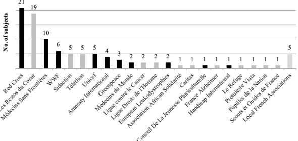
Bequests are presented as donations to a charity. Indeed, at the end of phase A, each subject is asked to indicate—through Web search—a charity to which he/she would like to donate part of the earnings he/she would eventually get in phase B. A short charity-related questionnaire follows. Our auxiliary assumption is that answers to this questionnaire provide a measure of the subject’s utility from the act of giving to the charity in phase B. Donations to the charities are implemented by the experimenter within 24 hours by the end of the experiment, with each subject getting private E-mail confirmation of his/her own donation.
This feature of the design has two main advantages. On the one side, it allows us to create a tie between the donor and the bequest’s receiver, which it would not be the case if the latter were a randomly matched subject in the lab. On the other side, it avoids undesired e↵ects of post-experiment bequest sharing and unreliable measures of warm-glow altruism if the receiver were a relative or a friend of the experimental participant.
After Andreoni’s (1989) model of warm-glow altruism, several experimental studies have confirmed that warm glow is an important factor in monetary donations to a charity (for a review, see Brown et al. 2013). In particular, Crumpler & Grossman (2008) show that agents give some of their own money to charity even when their donation does not alter the total amount donated to the charity. That is, individuals are giving for pure warm-glow reasons, not to expand the amount available to the charity.
Some experiments have been run about how donors’ behavior extends to environments with uncertain income. This literature is relevant for our experiment, since in phase B of our design subjects choose the amount of the bequest in period 2 through the strat-egy method, i.e., before the uncertainty about “survival” and the income in period 2 is resolved. In this regard, Kellner et al. (2015) have proved that it is cheaper to commit to donate to a charity before the uncertainty is resolved, and so a larger donation is required to maintain a positive image. This result is in line with Converse et al. (2012), who find that the combination of wanting an outcome and lack of control under uncertainty increases donations to charity, and suggest that this is due to a belief that one’s donations increase the likelihood of the desirable outcome. For all these reasons, we should expect elicited bequests in phase B of our experiment to be larger than theoretically predicted. However, this e↵ect is compensated by the fact that in our annuity-charity decision prob-lem, charities receive a (involuntary) bequest also in the case of “no survival” in period
2, namely the amount invested in bonds in period 1. Thus, the above-mentioned behav-ioral distortions on the voluntary bequest in the favorable state of the world should be mitigated by the possibility of an involuntary bequest in the unfavorable one.
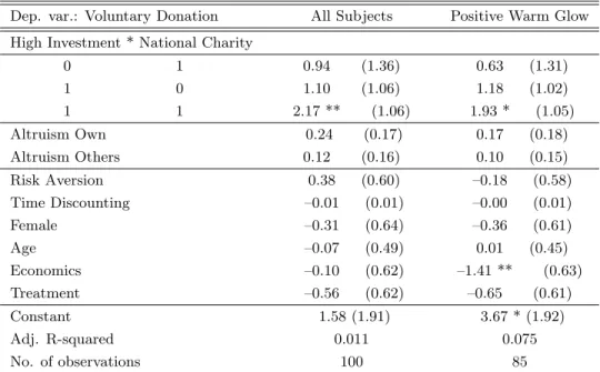
Our experimental results confirm the theoretical prediction of a negative impact of ambiguity aversion and a positive impact of ambiguity proneness on the demand for an-nuities. Indeed, in period 1, ambiguity-averse subjects invest significantly less in annuities than ambiguity-neutral ones, and ambiguity-loving subjects invest significantly more than the latter. Furthermore, warm-glow altruism and giving play no significant e↵ect on the demand for annuities.
In period 2, as assumed in our theoretical framework, we find that the way the subject shares his/her financial wealth if active is independent from his/her ambiguity attitude. In line with the theory, we observe that the amount the subject decides to keep for him/herself is increasing in the annuities purchased in period 1. However, the subjects’ bequest to the chosen charity is non-decreasing in the investment in annuities. We find it increasing only for those subjects donating to charities which they perceive as “closer” in terms of own participation and/or involvement, thereby experiencing a sufficiently high level of warm-glow altruism through their voluntary donation.
The rest of the paper is structured as follows. Section 2 presents our model of an-nuitization and bequest under ambiguous survival probabilities. Section 3 describes the experimental design, discusses our operational measure of ambiguity attitude, and presents our experimental hypotheses. Section 4 presents and discusses our experimental results in light of the theoretical predictions. Section 5 concludes by framing our contribution within the experimental literature of self-insurance decisions. An Online Appendix collects technical details about the theoretical analysis (Online Appendix A), the experimental in-structions (Online Appendix B), and the data analysis (Online Appendix C).
2
A model of annuitization with ambiguity and bequest
This section applies the recent rationale for ambiguity proposed by KMM to a static model of consumption and bequest under uncertain lifetime similar to Yaari (1965) and Davido↵ et al. (2005).
The length of life is at most two periods with the second one being uncertain. The Decision Maker (DM, hereafter) derives utility from a bequest that might happen at the end of periods 1 and 2 and, upon survival, from consumption in period 2. At the first period, the DM is endowed with an initial positive income w that can be shared between bonds and annuities. Bonds return R > 0 units of consumption in period 2, whether the DM is alive or not, in exchange for each unit of the initial endowment. Conversely, annuities return Ra R in period 2 if the DM is alive and nothing if she is not alive. Due
to the possibility of dying, the demand for bonds should be non-negative. If alive during the second period, the DM may allocate her financial wealth between consumption and bequest. Since death is certain at the end of period 2, the latter is exclusively a demand for bonds.
We denote by a, the demand for annuities and by w a, the demand for bonds, decided in period 1. Moreover, let c and x denote respectively the consumption and the bequest
decided in period 2. The budget constraint in period 2 if the DM is alive writes:
c = Raa + R(w a) x, (1)
and the non negativity constraints are:
c 0, x 0, a w. (2)
Following Davido↵ et al. (2005), we assume that whatever the length of the DM’s life, bequests are received in period 3, involving additional interest: the bequest is therefore xR, if the DM is alive in period 2, while it is (w a)R2, if she is not.
As in Yaari (1965) and Davido↵ et al. (2005), we assume that the DM’s state-dependent utility is separable: g[c] + h[xR] if alive in period 2 and h[(w a)R2] if she is not alive.4
Importantly, we assume that survival probabilities are uncertain. More precisely, the DM does not know her own probability distribution but only knows the set of possible distributions. There exist states of nature associated with given survival probabilities that may be interpreted as health types, to which the DM subjectively associates a probability to be in. Ambiguity is hence modeled as a second-order probability over first-order proba-bility distributions. Let us denote the random (continuous or discrete) survival probaproba-bility byp whose support is denoted Supp(e p), and the survival expectancy as it is evaluated bye the DM by E(p) = p. More precisely, given that it does not a↵ect the main results, wee suppose that the principle of insufficient reason applies, and so p corresponds to the mean survival probability E(p).e
We also assume that the DM has smooth ambiguity preferences. Following KMM, ambiguity attitude is introduced using a function , a von Neumann-Morgenstern index function accounting for the attitude toward mean preserving spreads in the induced dis-tribution of the lifetime expected (state-dependent) utility conditional to the unknown survival probability p. Therefore, the DM’s ex-ante utility is given by an expectatione of an expectation (see KMM, p. 1851, Eq. (1)). The inner expectations evaluate the expected utilities corresponding to possible first-order probabilities while the outer expec-tation aggregates a transform of these expected utilities with respect to the second-order prior. The function determines ambiguity attitude of the DM in the sense that a concave (resp: convex) implies an ambiguity-averse (resp: ambiguity-loving) DM.
To implement a theory-driven laboratory experiment, we parametrize the annuity-bequest two-period decision problem as follows: p = 1/2, w = 10, R = 1, and Ra = 2.
With this parametrization, Ra = R/p, i.e., the annuities available for purchase are
actuarially fair, as it is assumed in Yaari (1965). Furthermore, since R = 1, purchase of bonds is equivalent to transferring wealth across periods.5 The two-stage uncertainty
in the KMM framework is implemented with discrete first-order survival probabilities with Supp(p) =e {0, 1/10, 2/10, ..., 1}, and discrete second-order probabilities over Supp(ep).
4The twice continuously di↵erentiable functions g and h are supposed to be positive, increasing and
strictly concave. They also satisfy g[0] = h[0] = 0, and lim
%!0g
0[%] = lim
%!0h
0[%] = +1.
5In Sections 3.2.2 and 3.2.3, we will explain how the latter feature greatly simplifies the computational
More precisely, call p✓ = ✓/10 the unknown first-order probability, with ✓2 {0, 1, ..., 10}.
Call q✓ the corresponding second-order probability.
With this, the lifetime expected utility of the second-stage lottery in period 1, denoted U(a, x, p✓), is the realization of the random variableU(a, x, ep) in the state of the world ✓
that, for ✓2 {0, 1, ..., 10}, writes: U(a, x, p✓) = p✓
⇣
g[10 + a x] + h[x]⌘+ (1 p✓)h[10 a], (3)
and the ex-ante utility function writes
1(
10
X
✓=0
q✓( (U(a, x, p✓)))), (4)
where the twice continuously di↵erentiable function is assumed to be increasing. The DM faces the following annuity-bequest decision problem, denotedP :
max a,x 1( 10 X ✓=0 q✓( (U(a, x, p✓)))) (5) s.t. 10 + a x 0, x 0 and a 10.
Then, upon existence, the solution (a?, x?) of P satisfies the FOCs: 10 X ✓=0 q✓ ⇣ 0(U(a?, x?, p ✓)) h p✓ ⇣ g0[10 + a? x?] + h0[x?]⌘ (1 p✓)h0[10 a?] i⌘ = 0, (6) g0[10 + a? x?] + h0[x?] = 0. (7) We remark that the survival probability p✓ a↵ects the optimal demand for annuities
but not, as shown by equation (7), the optimal allocation of the financial wealth between consumption and bequest. Furthermore, condition (7) can be used to define the application x? = f (a?), which satisfies 0 f0(a?) 1. Hence, at the optimum, if the DM survives, her bequest f (a?) and her consumption 10 + a? f (a?) increase with the demand for
annuities a?. All this is formally stated in Proposition 1 (see Online Appendix A for the formal Proof).
Proposition 1. (i) Upon survival, the optimal share between bequest x? and
con-sumption c? = 10 + a? x? does not depend on the ambiguity attitude of the DM. (ii)
Upon survival, (voluntary) bequests x? and consumption c? increase with the optimal demand for annuities a?.
If the trade-o↵ between consumption and bequest if alive—i.e., the DM’s warm glow— is not a↵ected by the ambiguity attitude of the DM, it is clear, from equation (6), that the ambiguity attitude plays a crucial role to determine the demand for annuities. We can establish that:
Proposition 2. The optimal demand for annuities a? which solves the problem P : (i) is positive and denoted a?0 if the DM is ambiguity-neutral; (ii) is lower than a?0 if the DM is ambiguity-averse; (iii) is larger than a?
0 if the DM is ambiguity-loving.
Here we provide a qualitative explanation of Proposition 2 based on intuition (see Online Appendix A for the formal Proof). Ambiguity attitude determines the optimal exposure to uncertainty. An ambiguity-averse DM chooses to be less exposed that an ambiguity-neutral DM, which means that she aims at smoothing the expected utilities computed in each state of nature. This can be achieved by reducing the share of annuities in the portfolio.
Let us point out that this result may not be so “trivial”, as one may erroneously think an annuity as an insurance product whose demand should increase with the aversion to uncertain lifetime. Let us now explain why this is not the case by considering only two states of nature, e.g., ✓ 2 {1, 9}, for which the survival probabilities are respectively p1 = 1/10 and p9 = 9/10. Using equation (3), the optimal di↵erence of expected utilities
in both states is thus:
(p9 p1)
⇣
g[10 + a? x?] + h[x?] h[10 a?]⌘, (8) which is proportional to the optimal di↵erence between the utility if the DM lives for two periods and the utility if she lives for one period only. As the utility depends on the bequest, the sign of the latter di↵erence is not a priori given. However, it can be proven that the latter di↵erence is always positive, and that reducing the demand for annuities reduces di↵erence (8). The intuition is that, upon survival, the utility increases with the share of annuities in the portfolio. As a consequence, to reduce the exposure to life uncertainty, an ambiguity-averse DM has to increase her demand for bonds, and reduce her demand for annuities. Conversely, an ambiguity-loving DM would prefer to increase the exposure to life uncertainty, by increasing the di↵erence (8) and, consequently, by reducing her demand for bonds and increasing her demand for annuities.6
3
An experimental test with charitable giving
3.1 The experimental protocol
Participants were 100 students of University of Strasbourg (60 male, 40 female; 67 under-graduate, 33 graduate; 70 in Economics, 7 in other Social Sciences, 9 in Human Sciences, and 14 in Natural Sciences). The experiment was run at the Laboratory of Experimental Economics of Strasbourg (LEES). Students were recruited through ORSEE (Greiner 2015). Four sessions of 25 subjects each were conducted at the LEES. Each person could only participate in one of these sessions. The experiment was programmed and implemented using the platform www.econplay.org of the LEES.
6The limit case such that the ambiguity aversion is infinite, was studied by d’Albis & Thibault (2012,
2018). It reveals that there exists a threshold above which the demand for annuity is nil when negative annuitization is not allowed.
Average earnings were e22.57, including an average transfer of e4.00 to a charity chosen by each participant during the experiment, as it will be explained below. The average duration of a session was 70 minutes, including instructions and payment.7
3.2 The experimental design
The experimental design is made of two phases (A and B), always implemented in the same order. Instructions of phase B are given and read aloud only prior to that phase.
Table 1 o↵ers a schematic representation of the experimental design, summarizing its main features and how the 100 subjects are funneled through the two orders of presentation of tasks of phase A. In particular, among the four sessions with 25 participants each, two sessions are implemented with the main treatment 1-2-3-4 (the order of tasks shown in Table 1), and other two with the order treatment 4-3-2-1. Subjects voluntarily enrolling for the experiment are randomly allocated to one of the four sessions, hence half of them to a 1-2-3-4 session, and the other half to a 4-3-2-1 session.
Table 1. Experimental design: main features
Phase A is meant to elicit a subject’s ambiguity attitude within the smooth ambi-guity model of KMM, in a battery of portfolio choice problems with ambiguous returns. This portfolio choice elicitation method is obtained as a combination of two well-known experimental designs: Halevy (2007) elicitation of lottery certainty equivalents (tasks 1 and 2), and Eckel & Grossman (2002) ordered lottery selection (tasks 3 and 4). Ambi-guity characterizes tasks 2 and 4 of phase A. Following Attanasi et al. (2014), behavior in tasks 1 vs. 2 discloses value-ambiguity attitude, and behavior in tasks 3 vs. 4 dis-closes choice-ambiguity attitude. Coherence (equivalence) between the two attitudes is a necessary condition implied by the smooth ambiguity model of KMM.
Phase B is meant to elicit subjects’ investment in annuities in a life-cycle framework `
a la Davido↵ et al. (2005), where the annuity vs. bond decision is taken in period 1, and a bequest (donation to a charity) is chosen in period 2 and implemented in period 3 (i.e., after the end of the experiment). This two-period investment-donation decision problem is the experimental implementation of the static decision problem of consumption and bequest under uncertain lifetime theoretically analyzed in Section 2. In particular, the investment problem of period 1 is an extension of Gneezy & Potters (1997) betting game to a situation where the subject is also uncertain about whether he/she can manage the money earned in period 1. Ambiguity characterizes period 1: the probability that the subject will be active in period 2 is unknown.
A final questionnaire about some idiosyncratic features is submitted at the end of the experiment. Each subject is asked his/her gender, age, year and field of study, and a question about self-assessment of time discounting.8
As for the experimental payment, at the end of the experiment, after the subject’s earnings and charity donation in phase B are determined, one of the four tasks of phase A is randomly selected and performed, thereby determining subject’s earnings from phase A. Then, the sum of subject’s earnings from phase A and from phase B is individually paid in cash. The subject’s donation to the charity in phase B, if any, is implemented by the experimenter immediately after the end of the experiment, and the donation receipt sent to him/her within 24 hours after the end of the experiment.
In the next two subsections, we present the specific design features of phase A and phase B, separately. In the last subsection, we discuss more in depth some key features of our design.
3.2.1 Phase A
Phase A is made of tasks 1-4, presented in reverse order in half of the sessions (50 subjects for each order). At the end of the experiment, only one of the four tasks is randomly selected and actually performed, so as to determine earnings of phase A.9 Instructions of
a new task are given and read aloud only prior to that task.
Task 1 is a choice between a lottery with known probabilities and a battery of ten fixed amounts of money, presented on ten consecutive lines (see Screen 1 in Online Appendix B). More precisely, each subject is given two options, Left and Right. Option Left is a lottery L1 with two outcomes, e0 and e20, and 50% probability each—10-ball urn with 5 yellow balls and 5 blue balls—i.e., L1 = (20, 0.5; 0, 0.5).10 Option Right gives instead
8This is a standard one-year matching question (see, e.g., Thaler 1981) under a “delay premium”framing
`
a la Loewenstein (1988): “You have the possibility to receive immediately e100 for your leisure. How much money do you need in order to give up on spending the e100 today and carry them over to the next year?”, the set of possible answers being integer numbers from 0 to 100. Thus, the higher the selected number, the lower the willingness to accept a delayed payment, and so the higher the intertemporal discount rate.
9More precisely, at the end of the experiment one of the subjects is asked to make a random draw
from an envelope containing four numbers. The drawn number (1, 2, 3, or 4) indicates the number of the task that is performed for all subjects in the session: the computer randomly selects a ball from the urn associated to this task. The color of the randomly selected ball is used to determine all subjects’ earnings.
10Before the experiment starts, each subject is asked to choose one of two colors: yellow or blue. The
a sure amount eXi, with Xi being an odd number with min X1 = 1, max X10 = 19,
and Xi = Xi+1 2 for each i = 1, ..., 9. For each of the ten Xi, the subject is asked to
indicate whether he/she prefers Left or Right. In particular, monotonicity is exogenously imposed: the subject is asked to choose the lowest Xi for which he/she prefers option
Right to option Left.11 Call this value X1, where the superscript indicates task t = 1. Subject’s earnings: If task 1 is the randomly selected task at the end of the experiment, the computer randomly draws one of the ten amounts Xi 2 {1, 3, ..., 19} (same for all
subjects, with each Xi having the same probability to be drawn). If, for this randomly
drawn amount ˜X1
i, the subject has indicated that he/she prefers option Left, i.e., ˜Xi1 <
X1, then lottery L1 is played: one of the ten balls is randomly drawn by the computer,
and his/her earnings are e20 (e0) if the ball is yellow (blue). If for ˜Xi1 the subjects has indicated instead that he/she prefers option Right, i.e., ˜X1
i X1, his/her earnings are
˜ X1
i, i.e., the randomly drawn amount.
Task 2 is the same as task 1, apart from the fact that here option Left is a lottery L2
(the superscript indicating task t = 2) with the same two outcomes as L1 but unknown
probabilities, i.e., L2 = (20,p; 0, 1e p). More precisely, the 10-ball urn used for task 2e has an unknown composition of yellow and blue balls: p can take one of the eleven valuese in {0, 0.1, ..., 0.9, 1} (see Screen 2 in Online Appendix B, with option Left indicating an urn with 10 grey balls rather than the 5-5 yellow-blue balls urn of Screen 1). In fact, the composition of the ambiguous urn is the same for all subjects in a session. They are told that it was determined prior to the experiment by randomly drawing one of the eleven possible compositions of yellow-blue balls (0-10, 1-9, ..., 9-1, 10-0). Each composition had the same probability to be drawn, although subjects were not told about this. Call value X2 the lowest X
i for which the subject prefers option Right to option Left in task t = 2.
Subject’s earnings: If task 2 is the randomly selected task at the end of the experi-ment, ˜Xi2 is randomly drawn following the same procedure as for ˜Xi1 for task 1, and the comparison between ˜X2
i and X2 determines the subject’s earnings. However, if ˜Xi2 < X2,
and so lottery L2 is played, the random draw of a ball is made by the computer from the urn with unknown composition described above.
Task 3 is a choice among ten two-outcome lotteries L31, L32, ..., L310 (the superscript indicating task t = 3), with same known probabilities and same mean, presented on ten consecutive lines (see Screen 3 in Online Appendix B). As for task 1, a 10-ball urn with 5 yellow and 5 blue balls is used, so all lotteries are of type L3j = (xj, 0.5; xj, 0.5), with
xj = 10 + j and xj = 10 j, for j = 1, 2, .., 10. By construction, all lotteries have mean 10,
and standard deviation increasing in j, hence lowest for j = 1, i.e., for L3
1 = (11, 0.5; 9, 0.5),
and highest for j = 10, i.e., for L310= (20, 0.5; 0, 0.5). The latter coincides with L1 of task 1. Call choice j3⇤ the chosen line and L3j⇤ the chosen lottery in task 3.
Subject’s earnings: If task 3 is the randomly selected task at the end of the experiment, the computer randomly draws one of the ten balls of the urn with known composition (5 yellow balls, 5 blue balls). The subject’s chosen line j3⇤ in task 3 determines the played
the subject would play in the experiment with an urn with yellow and blue balls. From now on, the experimental design is explained under the assumption that the color chosen by the subject before the experiment starts is yellow. This is without loss of generality: the same rules of the decision problem also hold if assuming that the chosen color is blue, and inverting “yellow” with “blue” in what follows.
lottery L3j⇤: if the randomly drawn ball is yellow, the subject’s earnings are (10+j3⇤) euros;
otherwise, his/her earnings are (10 j3⇤) euros.
Task 4 is the same as task 3 (the ten lotteries L4j with j = 1, 2, ...10 have the same two outcomes as L3j for each j). However, outcome probabilities are unknown, i.e., L4j = (xj,p; xe j, 1 p). As for task 2, the 10-ball urn used for task 4 has an unknown compositione
of yellow and blue balls: p can take one of the eleven values ine {0, 0.1, ..., 0.9, 1} (see Screen 4 in Online Appendix B, where an urn with 10 grey balls is shown, rather than the 5-5 yellow-blue balls urn of Screen 3). The composition of the ambiguous urn is the same for all subjects in a session. They are told that it was determined prior to the experiment by randomly drawing one of the eleven possible compositions of yellow-blue balls. Each composition had the same probability to be drawn (subjects were not told about this). The composition of the two urns of tasks 2 and 4 has been determined through two independent random draws. Call choice j4⇤ the chosen line and L4j⇤ the chosen lottery in task 4.
Subject’s earnings: If task 4 is the randomly selected task at the end of the experiment, di↵erently from task 3, the random draw of a ball by the computer is made from the urn with unknown composition described above.
At the end of phase A, none of the four tasks is actually performed. Subjects move directly to phase B.
3.2.2 Phase B
Phase B begins with the subject being asked to indicate a charity to which he/she would like to donate part of the earnings that he/she would get in the decision problem he/she will participate in phase B.12A short charity-related questionnaire follows. It is meant
to elicit the relation of the subject with the chosen charity13 and his/her perceptions of others’ and own altruism.14
The subject faces the choice of the charity and the related questionnaire before in-structions of the decision problem they will participate in phase B are distributed. They concern the following two-period investment-donation decision.
In period 1 the subject is given 10 euros and he/she has to decide how many of them to invest, where a2 {0, 1, ..., 10} is the invested amount and 10 a the amount not invested.
There are two possible outcomes in period 2 for the invested amount in period 1. These two outcomes are determined through a 10-ball urn with unknown composition of yellow and blue balls. Thus, it may contain from 0 to 10 yellow balls and from 0 to 10 blue balls. The composition of the urn, which is the same for all subjects, has been determined
12The subject is given 5 minutes to find the website of the chosen charity and copy-paste it on the screen
of the experimental software.
13The four questionnaire items are: “For how many years have you known this charity?”; “How many
times have you already donated to this charity?”; “Did you ever participate in the activities of this charity?”; “Is any of your relatives or friends directly concerned by this charity?”.
14The two questionnaire items are, respectively: “Would you say that most of the time people only care
about themselves or they try to help others?”; “Would you say that most of the time you only care about yourself or you try to help others?”. Possible answers to each question are on a scale from 0 (only care about oneself) to 10 (help others).
before the experiment by randomly drawing one of the eleven possible compositions of balls. Each composition had the same probability to be drawn, although subjects were not told about this. The composition of this ambiguous urn has been determined through a random draw independent from those made to compose the two ambiguous urns of task 2 and task 4 of phase A.
The random draw of a ball from the urn at the beginning of period 2 has two conse-quences. The first one concerns the subject’s earnings: if the drawn ball is yellow, then in period 2 the invested amount is multiplied by 2 (2a); if the drawn ball is blue, then in period 2 the invested amount is lost (0). The second one determines whether or not the subject is active in period 2:
- if the drawn ball is yellow, then the subject is active in period 2: his/her total wealth at the beginning of period 2 is the sum of the amount not invested and two times the invested amount, i.e., (10 a) + 2a = 10 + a euros. Then, in period 2 the subject chooses how much of this (10 + a) euros he/she wants to donate to the previously chosen charity (x) and how much he/she wants to keep for him/herself (10 + a x). Hence, x is the voluntary donation to the charity, i.e., conditional to the subject being active in period 2. - if the drawn ball is blue, then the subject is not active in period 2 (there is no choice he/she can make): the only amount that is not lost, i.e., the one not invested in period 1, (10 a) euros, is directly donated to the previously chosen charity. This is the involuntary donation to the charity, i.e., conditional to the subject not being active in period 2.
To summarize, if a yellow ball is randomly drawn at the beginning of period 2, the subject’s earnings in phase B are (10 + a x) and the donation to the charity is x, with x being chosen by the (active) subject in period 2; otherwise, the subject earns nothing in phase B and the donation to the charity is (10 a), with this donation not being chosen by the (inactive) subject in period 2.
After the instructions of the two-period investment-donation decision problem have been read aloud by the experimenter, the subject is asked to go through two sets of four control questions, aimed at stating his/her comprehension of the decision problem. Each set of questions involves an example of (a, x) choice, and questions about the sub-ject’s earnings and the voluntary/involuntary donation to the charity for each color of the randomly-drawn ball.
Then, period 1 of the decision problem is performed: the subject chooses the invested amount a. At the end of period 1, the subject chooses x, according to a strategy method : he/she indicates the amount of the voluntary donation to the charity before knowing whether he/she will be actually active in period 2, i.e., before the random draw of the ball from the ambiguous urn. Phase B ends with this random draw, same for all subjects, and the determination of subject’s earnings from phase B and his/her donation to the charity. The subject’s voluntary or involuntary donation to the charity, if any, is implemented by the experimenter immediately after the end of the experiment, and the donation receipt sent to him/her within 24 hours after the end of the experiment. This last step of the design can be interpreted as period 3 of phase B,15 where the experimental subject is no
more active, independently from his/her choices and random events in periods 1 and 2.16
15Recall that in the model of Section 2 bequests are received in period 3.
3.2.3 Comments on the experimental design
In this section we comment on some important features of the experimental design, and provide motivations for specific design choices.
Several design features of phase A deserve to be discussed:
(A.1) Other relevant designs. Besides the one of Halevy (2007) from which our phase A takes inspiration, other designs might be used to elicit ambiguity attitude within a KMM framework. We quickly present some of the most well known, in a chronological order. Chakravarty & Roy (2009) use as experimental instrument a multiple price list method (comparable to our tasks 1-2), able to disentangle risk attitude and ambiguity attitude, and to capture di↵erences in behavior under uncertainty over gains vs. losses.
Ahn et al. (2014) simulates a standard portfolio problem, more framed than our tasks 3-4: the subject has to allocate his/her wealth among three assets under a budget constraint. Each asset pays depending on the color of the ball drawn from an Ellsberg-like 3-color urn. The prices of assets are exogenously varied. Unlike our task 4, where the exposure to ambiguity is fixed by the experimenter, in their design subjects can reduce exposure to ambiguity by choosing portfolios with payo↵s less dependent on the ambiguous states. Baillon & Bleichrodt (2015) propose choices between a binary lottery and a binary act, for di↵erent known probabilities of the lottery outcomes and the same level of ambiguity of the act. From these choices, they elicit the matching probabilities, respectively for an event and its complement, making the subject indi↵erent between the lottery and the act. Cubitt et al. (2018) propose an experiment where each subject’s ambiguity sensitivity is measured by an ambiguity premium, a concept analogous to and comparable with a risk premium. As in our design and in the one of Chakravarty & Roy (2009), also in their design some tasks feature choice under risk and others choice under ambiguity. With this approach, they are able to calculate ambiguity premia within KMM. A distinctive feature of this approach is the estimation of each subject’s subjective beliefs about the uncertainty in ambiguous tasks. Di↵erently, we adopt a more qualitative approach to testing, as also Halevy (2007), Baillon & Bleichrodt (2015), and the following study do.
Cubitt et al. (2019) use specially constructed decks of cards, divisible into the four stan-dard suits. Subjects are told that there would be equal numbers of black and red cards in each deck, but not exactly how the black cards would subdivide into clubs and spades, nor how the red cards would subdivide into hearts and diamonds. In each case, the com-positions are determined by drawing from a bag containing two types of balls, the relative proportions of which are unknown to subjects. This approach di↵ers from the one by Baillon & Bleichrodt (2015) by its use of indi↵erences expressed on a monetary scale, rather than on a probability scale, to indicate preferences. A key feature of their design is the possibility to manipulate whether the compositions of black cards and red cards are mutually dependent or mutually independent. A feature that might turn useful to analyze an extension of our study that we propose in the Conclusions, namely one in which also
the Instructions) “Immediately after having privately paid all subjects’ earnings, the experimenter will go through the charity’s website indicated by each subject at the beginning of phase B, make the on-line donation and fill in the donation screen with the identity of the donor; the email confirmation of the electronic donation will be privately forwarded by the experimenter to the subject within 24 hours after the end of the experiment, so as to account for possible delays due to any charity’s website problems.”
bonds are ambiguous, with this ambiguity correlating with the one of annuities.
(A.2) Order treatment. As in Halevy (2007), we also implement an order treatment. The goal is to check whether subjects’ elicited ambiguity attitude is influenced by either pre-senting ambiguous tasks before unambiguous ones—task 2 (4) before task 1 (3)—and/or presenting choice-ambiguity tasks (3 and 4) before value-ambiguity tasks (1 and 2).17
(A.3) Avoidance of subject’s suspicion on the composition of the ambiguous urns. An important issue raised in the experimental literature about Ellsberg-type tasks is sub-jects’ thinking about strategic behavior and/or manipulations by the experimenter (see Schneeweiss 1973, Kadane 1992). To prevent the possibility that subjects might suspect they can be tricked on computer-generated realizations of random processes, we imple-ment a combination of three features. First, for the each of the three ambiguous tasks (phase A task 1, phase A task 2, and phase B period 1), we determine the yellow-blue balls composition of the urn prior to the experiment, with independent random draws for each urn. Second, given the ambiguous task, subjects are assigned the same randomly generated urn composition. Third, at the beginning of the experiment we let each subject choose one of two colors (yellow or blue). The chosen color is associated to the highest of the two outcomes for each lottery that the subject would play in the experiment with a computerized urn with yellow and blue balls. The fact that the chosen “winning” color is not the same for all subjects should prevent the possibility of strategic manipulations of the computer-generated realization by the experimenter.
(A.4) Minimization of across-task contamination in phase A. Although subjects are told that phase A is made of four tasks, as in Halevy (2007) and Attanasi et al. (2014) instruc-tions of a new task are given and read aloud only prior to that task.
(A.5) Minimization of across-task and across-phase hedging behavior against ambiguity (see, e.g., Bade 2015). During and at the end of phase A, subjects know nothing about the composition of the ambiguous urns of tasks 2 and 4: the random draws for phase A are performed only at the end of the experiment. This prevents subjects from making any updating about the actual composition of the second ambiguous urn shown in phase A (task 4 in the main treatment and task 2 in the order treatment) and of the ambigu-ous urn of phase B. Moreover, such updating would be meaningless, since the random draws determining the composition of the three ambiguous urns have been independently performed before the experiment.
Several design issues of phase B deserve to be discussed:
(B.1) Simpler decision problem. In the experiment, the labels “annuity” and “bond” are never used in the instructions, so as to avoid framing e↵ects. We use the more neutral wording “invested amount” and “amount not invested”, respectively. This, coupled with a return on bonds set equal to 1 in the experiment, allows us to present the subjects with a simple investment problem where the invested amount a is the demand for annuities and
17The only significant order e↵ect found in Halevy (2007) with four randomized orders of urns is that
the task presented as first received a significantly lower reservation price than under alternative orders in which this urn was not the first, independently of the task. Therefore, we thought that having a “value & unambiguous”task shown at first in the main treatment (as in Halevy 2007) and the opposite (in both type and information) “choice & ambiguous”task shown at first in the order treatment would have represented the right counterbalance.
the amount not invested (10 a) is the demand for bonds. The fact that the demand for bonds is a pure transfer of the initial endowment from period 1 to period 2 is without loss of generality, given that in the general version of the annuity-bond trade-o↵ problem, the return on bonds is independent of whether the subject is “alive” (active) or not in period 2 (see d’Albis & Thibault 2018). Furthermore, the experimental implementation of the three periods of phase B is in line with the return on bonds being set equal to 1. In fact, the time lag between period 1 and period 2 is very short (period 2 starts immediately after the end of period 1). Same is for period 2 and period 3 (bequest implementation): the experimenter implements the subject’s bequest immediately after the end of the experi-ment, and the bequest receipt is sent to the subject within 24 hours (same short time lag between bequest decision and bequest implementation for all subjects in the experiment). As a final remark on this point, we acknowledge that this “invest” vs. “not invest” frame might induce an experimenter demand e↵ect: experimental subjects could see in the act of commission (invest) rather than in the act of omission (not invest) cues that the former constitutes appropriate behavior. However, as Zizzo (2010) correctly states, the exper-imenter demand e↵ect is a potential problem only when it is positively correlated with the true experimental objectives predictions. And, in our case, the e↵ect goes against under-annuitization, which is our prediction in Section 2 for ambiguity-averse subjects. (B.2) Bequests as charity donations. In the model of Section 2, the subject’s voluntary bequest x is the money donated to the next generation if “alive” in period 2, and the in-voluntary bequest (10 a) is the money left to it if not “alive” in period 2. The subject’s warm-glow intergenerational altruism is captured by h(x) and h(10 a), respectively in the case where he/she is alive or not alive in period 2. Recall that warm glow is a neces-sary condition to obtain under-annuitization (see Yaari 1965, and Davido↵ et al. 2005), which is the main object of our study. To induce a positive h(·) the experimental im-plementation, we try to relate the bequest’s receiver (outside the experiment, in period 3 of phase B) to the donor (in the experiment, in period 2 of phase B). In particular, we let subjects in the experiment indicate—before knowing the decision problem in phase B—a charity as bequest recipient.18 The fact that the subject’s bequest is implemented— immediately after the experiment—by the experimenter (who provides the subject with the charity donation receipt) guarantee ex-post check of bequest implementation. Finally, the charity-related questionnaire allows us to measure, among other things, the subject’s links with the chosen charity and thereby his/her level of warm-glow altruism toward it. (B.3) Strategy method for voluntary bequest elicitation. In a life-cycle framework theo-retically analyzed in Section 2, the voluntary bequest choice x is made in period 2, and only if the subject is “alive,” i.e., active, in period 2. However, following a widely-used method in experimental economics, in the experiment each subject is asked to choose x before period 2. This allows us to elicit x also for those subjects who will not be active in period 2, due to an unfavorable random draw at the end of period 1.19
18We decided not to involve a subject’s relative or friend as bequest receiver, mainly for two reasons:
first, it would not have been possible to check ex-post the exact sharing of the subject’s bequest between his/her relative or friend and him/herself; second, measuring the subject’s altruism toward a relative or friend would have lead to similarly high levels of elicited altruism in the subject pool, with no heterogeneity in the distribution of this idiosyncratic feature.
(B.4) Control questions. The two sets of four control questions about the decision prob-lem in phase B are aimed at identifying subjects for whom we are sure that they have not perfectly understood the rules and/or the structure of payo↵s of the decision problem in phase B. We include in this group all subjects that have made at least 1 mistake in the first set and at least 1 mistake in the second set of 4 control questions. Although these subjects are allowed to participate in the two-period investment-donation decision problem, we do not consider them in the data analysis of phase B (Section 4.4).
Finally, our Payment protocol deserves some comments:
(P.1) Random-lottery incentive mechanism and accumulated earnings. In phase A, only one of the four tasks is randomly selected at the end of the experiment to determine subjects’ earnings in that phase. Here we adopt a random-lottery incentive mechanism— extensively used in economic experiments (see the survey in Cox et al. 2015)—with the twofold goal of obtaining no wealth e↵ect between di↵erent tasks of phase A, and propos-ing bigger stakes to experimental subjects. Furthermore, in order to let subjects focus separately on each phase of the experiment, we paid earnings of both phase A and phase B, thorugh two independent random draws. This payment protocol should have minimized potential distortions linked to the random-lottery incentive mechanism in phase A, in line with recent findings in the experimental literature (Cox et al. 2015).
(P.2) Phase A proposed before but paid after phase B. We propose to subjects phase A always before phase B, so as to avoid investment and bequest decisions in phase B being distorted by weird expectations about what will be the experimental task(s) in subsequent phase A. However, we pay phase A always after subjects go through and are paid for phase B, so as to minimize wealth e↵ects (e.g., heterogeneity of previously collected earnings) on behavior in phase B.20
3.3 The experimental hypotheses
In this section, first we show how the four tasks of phase A can be used to detect the sign of a subject’s ambiguity attitude within the KMM model. Then, building on the theoretical model introduced in Section 2, we derive two experimental hypotheses for phase B on, respectively, the impact of a subject’s elicited ambiguity attitude in phase A on his/her investment in annuities in period 1, and the e↵ect of the latter on his/her donation to the charity in period 2.
consumption if alive in period 2. However, the labels “bequest”, “consumption” and “alive” are never used in the instructions, again to avoid framing e↵ects. We use the more natural wording “amount donated to the charity” for x, “amount kept by the subject” for (10 + a x), and “active” rather than “alive”.
20We acknowledge that wealth e↵ects might not have been fully eliminated by design, since during phase
B subjects can expect positive earnings from phase A. If this were the case, then the restriction to constant ambiguity aversion in the KMM model (see KMM, p. 1876) would be more suited to the theoretical analysis of the ambiguous tasks in phases A and B. However, in Extension 2 of Online Appendix A we show that, ceteris paribus, the demand for annuities of an ambiguity-neutral subject increases in the additional endowment earned from phase A. Given that this additional endowment cannot be invested in phase B and is earned both if active and if not active in period 2 of that phase, the intuition leans towards a higher demand for annuities independently of the ambiguity attitude.
3.3.1 Elicitation of ambiguity attitudes in phase A
Recall that we use KMM’s smooth ambiguity model as a general framework. Therefore, as we already made for the theoretical framework of Section 2 implemented in phase B, we assume that also in phase A the subject’s preferences are represented by the von Neumann-Morgenstern Expected Utility function (henceforth, EU ) for simple lotteries, and we relax reduction between first and second-order probabilities in two-stage lotteries in order to account for multiplicity/uncertainty of the possible compositions of the second-stage lottery.
Each task of phase A (see Section 3.2.1) concerns two-outcome lotteries, i.e., with x, x2 R+, x > x. The urns with unknown composition of tasks 2 and 4 are represented
by the 10-ball one-stage lottery el✓ ⇠ (x, p✓; x, 1 p✓), where p✓ = ✓/10 is the first-order
probability given by the (unknown) ratio of the number of yellow balls ✓ 2 {0, 1, ..., 10} over 10 yellow and blue balls. The second-order probabilities over the composition of the 10-ball urn are q✓, with ✓2 {0, 1, ..., 10}, in both task 2 and task 4.
With this in mind, urns with unknown composition of tasks 2 and 4 can be modelled as a two-stage lottery Lt for t 2 {2, 4}, where the second stage is represented by a set of 11 lotteries el✓ ⇠ (x, p✓; x, 1 p✓), with x > x, and ✓ 2 {0, 1, ..., 10}. The first stage is
represented by the lottery Lt having as possible outcomes the 11 second-stage lotteries el✓
with probabilities (q0, ..., q10). These are the second-order probabilities over the plausible
probability distributions for el✓.
Following KMM, the subject’s ex-ante utility is measured, in tasks t2 {1, 2, 3, 4}, by:
u(CE(Lt)) = 1 10 X ✓=0 q✓ (EU (el✓)) ! (9) with EU (el✓) = p✓u(x) + (1 p✓)u(x). (10)
Function u is a von Neumann-Morgenstern utility function, and captures the sub-ject’s smooth ambiguity attitude. In fact, is a von Neumann-Morgenstern index function accounting for the attitude toward mean preserving spreads in the induced distribution of the expected utility of the one-stage lottery conditional to ✓, namely EU (el✓). KMM
show that “smooth ambiguity aversion” is equivalent to being concave. Therefore, it is equivalent to aversion to mean preserving spreads of the expected utility values induced by the second-order subjective probability and lottery el✓. Then, defining function v as
v = u, the certainty equivalent of the two-stage lottery of tasks t2 {1, 2, 3, 4} is:
CE(Lt) = v 1 10 X ✓=0 q✓v(CE(el✓)) ! , (11)
where CE(el✓) is the certainty equivalent of the one-stage lottery conditional to ✓. Function
v is a von Neumann-Morgenstern index function accounting for the attitude toward mean preserving spreads in certainty equivalents of the one-stage lottery conditional to ✓, namely CE(el✓) (see KMM 2005, p. 1855).
Note that the simple lottery of task 1 is analogous to a two-stage lottery with all second-stage lotteries el✓ being L1, and objective first-order probability p✓ = 1/2 for each
✓2 {0, 1, ..., 10}. Therefore, Eqs. (9) and (11) collapse to CE(L1) = u 1(EU (l
✓=5)), with
EU (l✓=5) = 0.5(u(20) u(0)) from Eq. (10). The same holds for the ten simple lotteries
of task 3 where, for each j = 1, 2, .., 10, the simple lottery L3j is analogous to a two-stage lottery with all second-stage lotteries el✓ being L3j, and, independently of j, p✓ = 1/2 for
each ✓ 2 {0, 1, ..., 10}. Therefore, for each j = 1, 2, .., 10, Eqs. (9) and (11) collapse to CE(L3j) = u 1(EU (l✓=5)), with EU (l✓=5) = 0.5(u(xj) u(xj)) from Eq. (10).
With all this in mind, by looking at the subject’s behavior in tasks 1-4, we can identify whether a subject shows aversion, neutrality or proneness to ambiguity within KMM. Let us first compare behavior in tasks 1 and 2.
In tasks 1 and 2, the subject is asked to value, respectively, the unambiguous lottery L1and the ambiguous lottery L2 with the same expected probability for the two outcomes of the second-stage lottery. In fact, the principle of insufficient reason suggests that the subject believes that each urn composition in task 2 is equally likely, as it actually was in the random composition of the urns prior to the experiment. Therefore, q✓ = 1/11 for each
✓ 2 {0, 1, ..., 10} because of the assumption of uniform distribution.21 Then, the third-order probabilities on parameter p yields E(p) = 1/2. As the two second-stage lotteries of tasks 1-2 have the same pair of outcomes (x, x) = (20, 0), their variety only depends on first-order probabilities. Thus, ambiguity aversion yields CE(L2) < CE(L1) in Eq. (11).
In Section 3.2.1 we called Xtthe lowest sure amount for which a subject prefers option
Right to option Left in task t2 {1, 2}. This Left-to-Right switching amount determines an interval estimate for the certainty equivalent of lottery CE(Lt) in task t2 {1, 2}: the greater Xt, the higher his/her estimated certainty equivalent. With this in mind, the
following operational definition of ambiguity attitude within KMM can be introduced. Definition 1 (value-ambiguity attitude)
A value-ambiguity-averse (loving) subject values an ambiguous lottery less (more) than its unambiguous equivalent with the same mean probabilities. Then, this subject shows value-ambiguity aversion if X2 X1, value-ambiguity neutrality if X2 = X1, and value-ambiguity proneness if X2 X1.
In short, a value-ambiguity-averse subject values an ambiguous lottery less than its unambiguous equivalent with the same mean probabilities. In the KMM model, this is true if the subject’s function is concave.
Our experimental design o↵ers an alternative to elicit ambiguity attitude by comparing the subject’s behavior in tasks 3 and 4. In tasks 3 and 4, the subject is asked to make a choice, respectively, among ten unambiguous lotteries L3j and among ten ambiguous lotteries L4j, for j = 1, 2, .., 10. Given j, the pair of outcomes (xtj, xtj) is the same for t2 {3, 4}, and—under the principle of insufficient reason—, in task 4 second-order prob-abilities q✓ = 1/11 for each ✓ and the expected probability for the two outcomes of the
second-stage lotteries L4j is E(p) = 1/2, the same as the objective probability of the two outcomes of the simple lottery L3j. Therefore, ambiguity aversion yields CE(L4j) < CE(L3j)
21See also Attanasi et al. (2014), who find that subjects’ elicited beliefs about the unknown composition
in Eq. (11) for each j = 1, 2, .., 10. Defining a dispersion order on the set of lottery indexes{1, 2, ..., 10}, such that 10 ... 2 1, a more dispersed lottery is equivalent to a portfolio containing a larger share invested in the risky asset.
In Section 3.2.2 we called jt⇤the subject’s chosen line in task t2 {3, 4}. The chosen line determines the dispersion (outcome spread) of the lottery Ltj⇤ played in task t 2 {3, 4}:
the greater the index jt⇤ (jt⇤ = 1, 2, ..., 10 for each t), the greater the dispersion of Lt
j⇤
t.
With this in mind, the following definition can be introduced. Definition 2 (choice-ambiguity attitude)
A choice-ambiguity-averse (lover) subject chooses a less (more) risky lottery when the probability distribution over lottery outcomes is ambiguous, with the same mean probability. Then, this subject shows choice-ambiguity aversion if j4 j3, choice-ambiguity neutrality
if j4 = j3, and choice-ambiguity proneness if j4 j3.
As anticipated above, in the KMM framework, “smooth ambiguity aversion” is shown to be equivalent to the concavity of the von Neumann-Morgenstern index function accounting for the attitude toward mean-preserving spreads in the induced distribution of the expected utility of the one-stage lottery conditional to the—in our experiment, 11—possible compositions of the unknown lottery. Gollier (2014) has shown that it is not true in general that the concavity of the function (value-ambiguity aversion) implies the choice-ambiguity-aversion of the subject. In other words, a value-ambiguity-averse subject could choose a lottery with greater outcome spread when probabilities are unknown (task 4) than when they are known (task 3).
However, Gollier (2014) provides sufficient conditions on the structure of the two-stage uncertainty to re-establish the link between the concavity of and ambiguity aversion. One of these sufficient conditions is that the di↵erent second-stage distributions of the lottery outcomes can be ordered by the Monotone Likelihood Ratio stochastic order.22 Referring to the ten lotteries Lt
j with j = 1, 2, .., 10 in tasks t = 3, 4, the set of distributions of
outcomes n(xt
j, p✓; xtj, 1 p✓)|✓ = 0, ..., 10
o
in the ambiguous task t = 4 can always be ordered by the Monotone Likelihood Ratio, for each j = 1, 2, ..., 10.23 Thus, we conclude
that, in the smooth ambiguity framework of KMM, the two operational definitions of value-ambiguity attitude and choice-ambiguity attitude are equivalent in the four tasks of phase A, and are satisfied if is concave. This justifies the following definition, which combines Definitions 1 and 2.
Definition 3 (coherent-ambiguity attitude)
A subject is coherent-ambiguity-averse if X2 X1 and j⇤
4 j⇤3, with at least one of the two
relations holding strictly; coherent-ambiguity-neutral if X2 = X1 and j4⇤ = j3⇤; coherent-ambiguity-loving if X2 X1 and j4⇤ j3⇤, with at least one of the two inequalities holding strictly.
22The monotone likelihood ratio property is a property of the ratio of two probability density functions.
Formally, distributions f (x) and g(x) bear the property if for every x > x, f (x)/g(x) f (x)/g(x), that is, if the ratio is nondecreasing in the argument x.
23In particular, they can be ordered from higher to lower ✓s. Start with f (x) = (x4
j, p10; x4j, 1 p10) and
g(x) = (x4
j, p9; x4j, 1 p9). Then, independently of j, f (xj4)/g(x4j) f (x4j)/g(x4j) since (1/0.9) > (0/0.1).
The same holds for every ✓ such that f (x) = (x4