Dwarfs or Giants? Stellar Metallicities and Distances from ugrizG Multiband Photometry

HAL Id: hal-02746882

https://hal.archives-ouvertes.fr/hal-02746882

Submitted on 9 Nov 2020

HAL is a multi-disciplinary open access

archive for the deposit and dissemination of

sci-entific research documents, whether they are

pub-lished or not. The documents may come from

teaching and research institutions in France or

abroad, or from public or private research centers.

L’archive ouverte pluridisciplinaire HAL, est

destinée au dépôt et à la diffusion de documents

scientifiques de niveau recherche, publiés ou non,

émanant des établissements d’enseignement et de

recherche français ou étrangers, des laboratoires

publics ou privés.

from ugrizG Multiband Photometry

Guillaume Thomas, Nicholaas Annau, Alan Mcconnachie, Sebastien Fabbro,

Hossen Teimoorinia, Patrick Côté, Jean-Charles Cuillandre, Stephen Gwyn,

Rodrigo Ibata, Else Starkenburg, et al.

To cite this version:

Guillaume Thomas, Nicholaas Annau, Alan Mcconnachie, Sebastien Fabbro, Hossen Teimoorinia,

et al.. Dwarfs or Giants? Stellar Metallicities and Distances from ugrizG Multiband Photometry.

The Astrophysical Journal, American Astronomical Society, 2019, 886 (1), pp.10.

�10.3847/1538-4357/ab4a77�. �hal-02746882�

Typeset using LA_{TEX twocolumn style in AASTeX62}

Dwarfs or giants? Stellar metallicities and distances in the Canada-France-Imaging-Survey from ugrizG multi-band photometry

Guillaume F. Thomas,1 Nicholaas Annau,2 Alan McConnachie,1 Sebastien Fabbro,1 Hossen Teimoorinia,1

Patrick Cˆot´e,1 Jean-Charles Cuillandre,3 Stephen Gwyn,1Rodrigo A. Ibata,4Else Starkenburg,5

Raymond Carlberg,6 Benoit Famaey,4 Nicholas Fantin,7 Laura Ferrarese,1Vincent H´enault-Brunnet,1

Jaclyn Jensen,7 Ariane Lan¸con,4 Geraint F. Lewis,8 Nicolas F. Martin,4Julio F. Navarro,2 C´eline Reyl´e,9

and Rub´en S´anchez-Janssen10

1_{NRC Herzberg Astronomy and Astrophysics, 5071 West Saanich Road, Victoria, BC, V9E 2E7, Canada} 2_{Department of Physics and Astronomy, University of Victoria, Victoria, BC, V8P 1A1, Canada}

3_{AIM, CEA, CNRS, Universit´e Paris-Saclay, Universit´e Paris Diderot, Sorbonne Paris Cit´e, Observatoire de Paris, PSL University,} F-91191 Gif-sur-Yvette, France

4_{Universit´e de Strasbourg, CNRS, Observatoire astronomique de Strasbourg, UMR 7550, F-67000 Strasbourg, France} 5_{Leibniz Institute for Astrophysics Potsdam (AIP), An der Sternwarte 16, D-14482 Potsdam, Germany}

6_{Departement of Astronomy and Astrophysics, University of Toronto, Toronto, ON M5S 3H4, Canada} 7_{Department of Physics and Astronomy, University of Victoria, Victoria, BC, V8P 1A1, Canada} 8_{Sydney Institute for Astronomy, School of Physics, A28, The University of Sydney, NSW 2006, Australia}

9_{Institut UTINAM, CNRS UMR6213, Univ. Bourgogne Franche-Comt´e, OSU THETA Franche-Comt´e-Bourgogne, Observatoire de} Besan¸con, BP 1615, 25010 Besan¸con Cedex, France

10_{UK Astronomy Technology Centre, Royal Observatory, Blackford Hill, Edinburgh, EH9 3HJ, UK}

(Accepted 10/02/2019)

Submitted to ApJ ABSTRACT

We present a new fully data-driven algorithm that uses photometric data from the Canada-France-Imaging-Survey (CFIS; u), Pan-STARRS 1 (PS1; griz), and Gaia (G) to discriminate between dwarf and giant stars and to estimate their distances and metallicities. The algorithm is trained and tested using the SDSS/SEGUE spectroscopic dataset and Gaia photometric/astrometric dataset. At [Fe/H]< −1.2, the algorithm succeeds in identifying more than 70% of the giants in the training/test set, with a dwarf contamination fraction below 30% (with respect to the SDSS/SEGUE dataset). The photometric metallicity estimates have uncertainties better than 0.2 dex when compared with the spectroscopic measurements. The distances estimated by the algorithm are valid out to a distance of at least ∼ 80 kpc without requiring any prior on the stellar distribution, and have fully independent uncertainities that take into account both random and systematic errors. These advances allow us to estimate these stellar parameters for approximately 12 million stars in the photometric dataset. This will enable studies involving the chemical mapping of the distant outer disc and the stellar halo, including their kinematics using the Gaia proper motions. This type of algorithm can be applied in the Southern hemisphere to the first release of LSST data, thus providing an almost complete view of the external components of our Galaxy out to at least ∼ 80 kpc. Critical to the success of these efforts will be ensuring well-defined spectroscopic training sets that sample a broad range of stellar parameters with minimal biases. A catalogue containing the training/test set and all relevant parameters within the public footprint of CFIS is available online.

Corresponding author: Guillaume F. Thomas guillaume.thomas@nrc-cnrc.gc.ca

Keywords: Distance measure; Red giant stars; Stellar photometry; Milky Way Galaxy; Milky Way stellar halo; Metallicity

1. INTRODUCTION

The advent of the European Space Agency’s Gaia satellite has yielded accurate proper motion for stars brighter than G ∼ 21 (Gaia Collaboration et al. 2018a). However, to transform this angular velocity into a tan-gential velocity, accurate distances are required. With the parallaxes measured from Gaia, the distances of the stars in the Solar vicinity can be measured with high precision out to a few kiloparsecs (sim 10% at 1.5 kpc). Despite this very impressive number, the distances of the large majority of the 1.3 billion stars present in the Gaia catalog cannot be accurately inferred using only Gaia parallaxes. For example, a main sequence star at 3 kpc has a parallax uncertainty of ' 10%, and at 7 kpc the uncertainty on the parallax is of the same order as the parallax measurement itself (Bailer-Jones et al. 2013; Ibata et al. 2017b). Therefore, distances to stars in the outer disc of the Galaxy and in the stellar halo cannot be accurately measured by direct inversion of the parallaxes (Bailer-Jones 2015;Luri et al. 2018).

Several methods have been developed to infer statisti-cally the distances of these stars using assumptions made on the global distribution of the stars in the Galaxy (e.g.

Bailer-Jones 2015;Bailer-Jones et al. 2018;Queiroz et al. 2018; Anders et al. 2019;Pieres et al. 2019). However, the actual distribution of stars in the Galaxy, especially in the stellar halo, is still not known precisely, and dif-ferent tracers yield difdif-ferent distributions (Thomas et al. 2018; Fukushima et al. 2019). Therefore, the correct prior to adopt on the “expected” distribution of the stars is not obvious. Moreover, the spatial distribution of stars found using distances estimated by these methods depends sensitively of the adopted prior (Hogg et al. 2018).

To overcome this problem, spectrophotometric meth-ods have been developed to infer stellar distances (e.g.

Xue et al. 2014; Coronado et al. 2018; McMillan et al. 2018; Queiroz et al. 2018;Hogg et al. 2018). However, these methods require expensive spectroscopic observa-tions. Moreover, the current generation of spectroscopic surveys do not exploit the full depth of Gaia. Juri´c et al.

(2008) and Ivezi´c et al. (2008) developed a method to estimate the distance and metallicity of stars using the SDSS u, g, r, and i bands that circumvents the need for spectroscopy. This method was revisited byIbata et al.

(2017b). Inherent to this method is the assumption that all stars are main sequence stars. Thus a giant with the same color as a main sequence star will be estimated to

be much closer than its true distance by several orders of magnitude.

To study in detail the chemical distribution and kine-matics of the outer disk, the complex structure of the stellar halo, and the interface region between the disk and the stellar halo, it is crucial to measure the distance of the stars, including the giants, over the full depth of Gaia.

In this paper, we present a new technique to estimate distances and metallicities, that is based heavily on the methods of Juri´c et al. (2008); Ivezi´c et al. (2008) and

Ibata et al. (2017b), and which incorporates Machine Learning techniques. This fully data-driven algorithm first discriminates between dwarfs and giants based on photometry alone, and then estimates the distances and metallicities for each set using the same photometry. More specifically, we use multi-band photometry pro-vided by the Canada-France-Imaging Survey (CFIS), Pan-STARRS 1 (PS1) and Gaia. This dataset is pre-sented in Section2. The architecture of the algorithm and its calibration are detailed in Section 3. The ac-curacy and the biases of the algorithm are tested using independent datasets in Section 4. We apply the al-gorithm to 12.8 million stars in the CFIS footprint in Section5and use these data to map the mean metallic-ity of the Galaxy. Finally, in Section6, we discuss the applicability of this type of algorithm to future datasets, including LSST, and discuss the scientific opportunities it presents.

2. DATA

The photometric catalog used in this study (hereafter referred to as the main catalog) is a merger of the u-band photometry of CFIS (Ibata et al. 2017a), with the griz-bands from the mean PSF catalog of the first data release of PS1 (Chambers et al. 2016) (PS1), and the G-band from the Gaia DR2 catalog (Gaia Collabora-tion 2018)1. Spatially, the survey area is limited by the current coverage of CFIS-u (∼ 4000 deg2 of the north-ern hemisphere, eventually covering 10,000 deg2 _{at the}

end of the survey), since Gaia is all-sky and PS1 cov-ers the entire sky visible from Hawaii. Photometrically, the depth is limited by the Gaia G-band. The total and

1 The y-band from PS1 and the GB P and GR Pbands of Gaia are not used in this study because the large photometric uncer-tainties for stars fainter than G > 19.5 lead to large unceruncer-tainties in the derived photometric metallicities and distances.

Dwarfs or giants? 360 270 180 90 0 R.A. (deg) 0 30 60 90 Dec. (deg) _{NGC 6205} NGC 6341 NGC 5466 NGC 5272 NGC 2419 Draco dSph GD-1

Figure 1. Current footprint of the CFIS-u survey (blue areas) on an equatorial projection. The ∼ 2, 600 deg2 of the public

area of CFIS-u is shown by the light orange area. The grey lines show the Galactic coordinates with the solid lines showing the Galactic Plane and the Galactic minor axis. The different satellites within the footprint are used to validate the distance estimated by our algorithm on Section4.3are also indicated in the figure.

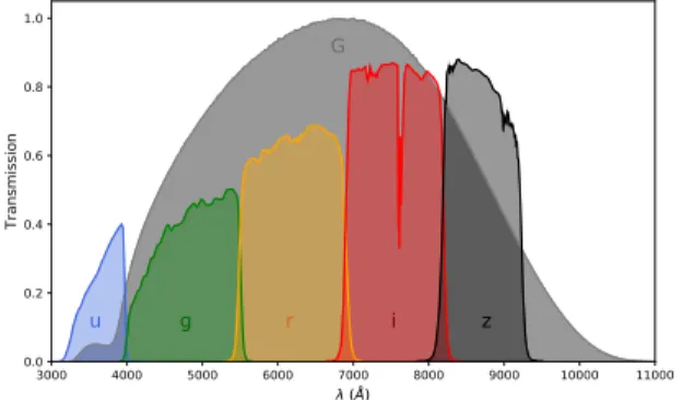
3000 4000 5000 6000 7000 8000 9000 10000 11000 λ (Å) 0.0 0.2 0.4 0.6 0.8 1.0 Transmission u g r i z G

Figure 2. The relative transmission of the photometric pass-bands used in this analysis.

public footprint of CFIS-u at the time of this analysis are shown in Figure1in blue and orange, respectively.

The normalized transmission of the different filters that constitute the main catalog are shown in Figure2. The different filters cover a range of wavelength from the near-UV to the near-IR (specifically, fromλ ' 3200 ˚A to 11000 ˚A). This large photometric baseline is useful to provide information on the overall shape of the spectral energy distribution (SED) of the stars, and we note that the overlap between different filters in some spectral re-gions, e.g. around 5500 ˚A, provides extremely valuable information in a short range of wavelength, compara-ble to extremely low-resolution spectroscopy. Indeed, it is expected that the absorption lines present in these overlap regions, such as the FeH-I and Ca-I, around 5500 ˚A, will have a stronger impact on the algorithm than other absorption lines located in the middle of a filter for which their signal is harder to disentangle from the rest of the SED. All of these features are put to-gether by the algorithm described in the next section to obtain dwarf/giant classification, the metallicity and the distance (absolute magnitude) of the stars.

For star-galaxy classification, we adopt the PS1 crite-ria, rPSF− rKr on < 0.05. As pointed out by as Farrow

et al.(2014), star-galaxy separation using this criterion become unreliable for stars fainter than rPSF = 21. Since

our catalog is effectively limited by the Gaia G-band lim-iting magnitude (G ' 20.7), the majority of our sources (more than 99.9 percent) have rPSF < 21. Therefore,

star-galaxy misclassification has negligible impact on the results of this study.

We use extinction values, E(B−V ), as given bySchlegel et al. (1998). The CFIS footprint is at relatively high Galactic latitude, |b| > 19◦, and most stars are moder-ately distant, so we can reasonably assume that all of the extinction measured in the direction of a star is in the foreground of the star. While this assumption is clearly hazardous for the closest stars, we will see be-low that it does not have a large impact on our results when we trace the chemical distribution of the disc of the Milky Way (see alsoIbata et al. 2017b). We adopt the reddening conversion coefficients for the griz-band of PS1 given by Schlafly & Finkbeiner(2011) for a re-denning parameter of Rv = 3.1. As in Thomas et al.

(2018), we assume that the conversion coefficient of the u-band of CFIS is similar to the coefficient of the SDSS u-band fromSchlafly & Finkbeiner(2011). For the Gaia G filter, we followSestito et al. (2019) by adopting the coefficient from Marigo et al. (2008) (based on Evans et al.(2018)).

3. METHOD 3.1. Overview

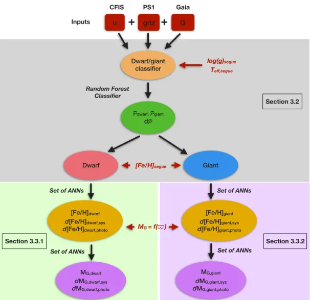
Figure 3 provides a schematic overview of the algo-rithm that we have developed. This algoalgo-rithm only uses the photometric data described in the previous section to first disentangle giants from dwarfs using a Random Forest Classifier (RFC) (Breiman 2001), as detailed in Section 3.2. Once this classification is done, two sets

Inputs CFIS u PS1 griz G Gaia

+

+

Dwarf [Fe/H]segue Giant

[Fe/H]dwarf

d[Fe/H]dwarf,sys

d[Fe/H]dwarf,photo

Pdwarf, Pgiant

dP

Set of ANNs Set of ANNs

MG,dwarf

dMG,dwarf,sys

dMG,dwarf,photo

Set of ANNs Set of ANNs

MG = f( )

$

Figure 3. Schema of the algorithm described in Section 3. The input parameters are the photometric measurements from

various surveys described in Section 2. Parameters in red are used for training. Dwarf - giant classification is done using

a Random Forest Classifier. For each class, a set of Artificial Neural Networks (ANNs) is used to compute the photometric metallicity. Then, another set of ANNs is used to compute the absolute magnitude in the G-band, which provides the distances to the stars.

of Artificial Neural Networks (ANNs), one for the stars identified as dwarfs (Section3.3.1) and another for the stars identified as giants (Section3.3.2), are used to de-termine the photometric metallicity. Finally, another two sets of ANNs are used to determine the absolute magnitude of the two groups of stars in the G-band.

To calculate the uncertainties on the different parame-ters estimated by our algorithm (PDwar f, PGiant, [Fe/H]

and M_G) caused by the photometric uncertainties of the different bands, we generate 20 Monte-Carlo realizations for each star. We also conducted 100 and 1,000 Monte-Carlo realizations for a sub-sample of 50,000 randomly selected stars. For these, we obtained final uncertain-ties that were typically< 1% different than what we ob-tained using only 20 realizations. As such, we proceeded with 20 Monte-Carlo realizations for the entire sample

in order to save expensive computational time. For each realization, we select a magnitude in each band from a Gaussian distribution centered on the quoted magnitude and with a standard deviation equal to the uncertainty on the magnitude. The uncertainties on the derived pa-rameters are set equal to the standard deviation for each parameter from these 20 realizations.

The CFIS-u footprint, which defines the spatial cov-erage of this study, includes a large number of stars ob-served by SDSS/SEGUE (Yanny et al. 2009b) and for which spectroscopic data are available. We use those stars with good quality spectroscopic measurements as training sets for the first two components of our algo-rithm. It is advantageous to use as large a training set as possible; therefore, we select 74, 442 SDSS/SEGUE stars present in the CFIS-u footprint that have a

spec-Dwarfs or giants? 0.0 0.5 1.0 1.5 2.0 2.5 3.0 (u-g)0 −0.50 −0.25 0.00 0.25 0.50 0.75 1.00 1.25 (g -r )0

Giants & Dwarfs

A-types

Figure 4. Color-color diagram of the SDSS/SEGUE stars that have SN R ≥ 25. The orange polygon corresponds to the locus of main-sequence and RGB stars in this color-color plane. This selection box removes A-type stars and white dwarfs from the subsequent analysis.

troscopic signal-to-noise ratio of SN R ≥ 25. This thresh-old was chosen because at lower SNR, the distribution of the uncertainties on the parameters given by the SEGUE Stellar Parameters Pipeline (SSPP) as a func-tion of the SNR is irregular, indicating that the parame-ters are poorly defined. Moreover, more than 96% of the stars with SN R< 25 have a parallax measurement with poor precision (> 20%) and these would not be used to calibrate the photometric distance relation even if they passed the SNR cut. For the third component of our al-gorithm (determination of the absolute magnitude), we use parallax information from Gaia (discussed later).

We first perform a color-color cut to remove A-type stars (which lie in the “comma-shaped” region in the color-color diagram of Figure4) and white dwarfs, that is defined by inspection of the Figure4and shown as the orange box. The presence of the Balmer jump in the u band for these stars means that they have a more com-plex photometric behavior compared to the other stars present in this color-color diagram, and the algorithms are significantly simplified if we remove them from con-sideration. We note that A-types stars in CFIS have been studied extensively in previous works (Thomas et al. 2018, 2019), and an analysis of the white dwarfs is in preparation (Fantin et al. in prep.). Imposing this color-color selection2on the SDSS/SEGUE spectra lead to a catalog of ∼ 42, 800 stars for which we have as-trometric, photometric and spectroscopic information.

2 The (u0− g0, g0− r0) vertices of this selection are : (0.64, 0.15), (1.0 0.15), (1.2, 0.3), (1.65, 0.4), (2.4, 0.74), (2.75, 0.97), (2.8, 1.02), (2.65, 1.08), (2.5, 1.05), (2.1, 0.83), (1.2 0.57), (0.95, 0.48), (0.7, 0.35).

This color-color cut represent the first step of our pro-cedure, and is applied to botht the test/training set and the final main catalog (see Section4.4).

3.2. Dwarf - giant classification

Here, we describe the method used to disentangle Red Giant Branch stars (RGBs) from main-sequence stars (MS)3. To perform this classification we use a Random Forest Classifier, whose inputs are the (u − g)0, (g − r)0,

(r − i)0, (i − z)0 and (u − G)0 colors normalized to have

a mean of zero and a standard deviation of one and the outputs are the probability of each to be a dwarf, Pdwar f, or a giant, Pgiant ≡ 1 − Pdwar f. It is worth

noting here that RFC does not necessary request a nor-malization of the inputs, but it is strongly suggested for an ANN. Therefore, to be consistent with the different steps of the algorithm, we use the normalized inputs for the dwarf/giant classification.

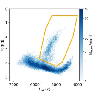
According to Lee et al. (2008), the typical internal uncertainties obtained by the SSPP on the adopted sur-face gravity (loggadop) is ∼ 0.19 dex. Therefore, we keep only the SDSS/SEGUE stars that have uncertain-tiesδ log(g) ≤ 0.2. The final SDSS/SEGUE catalog used to train/test the dwarf - giant classifier contains 41, 062 stars. This catalog is shown as a Kiel diagram in Figure

5, where we define the stars lying in the orange poly-gon as giants and all other stars as dwarfs. Note that we could in principle use Gaia DR2 parallax measure-ments to classify the stars as dwarfs or giants; however as we will show later, the parallax measurements of Gaia DR2 are not precise enough, especially for stars with [Fe/H] < −1.0, many of which are generally located at large distances and have poor parallax precision.

We note that our “giant” selection contains a large ma-jority of RGB stars but also sub-giants stars, with an effective temperature between 5000 ≤ Te f f (K) ≤ 6000

and surface gravity between 3.2 ≤ log(g) ≤ 3.9. Even on a Kiel diagram, it is hard to define a strict limit be-tween dwarfs, sub-giants and giants, especially when we include the uncertainties on the surface gravity which acts to blur any boundaries we adopt. The addition of a sub-giant class adds to the complexity of the algo-rithm and does not resolve the underlying problem of the “fuzzyness” between classes. For this reason, we do not consider a specific class of sub-giant stars. We also note that our definition of giants does not include the major-ity of Asymptotic Giant Branch stars (AGBs). However, there are very few AGBs in the SDSS/SEGUE catalog, and so we are unable to train the algorithm to identify

3 Hereafter, we refer to the RGBs as giants and to the MSs as dwarfs.

4000 5000 6000 7000 Teff (K) 0 1 2 3 4 5 lo g (g ) 1 3 5 10 30 50 Nst a rs /p ix e l

Figure 5. Kiel diagram showing the distribution of stars in the SDSS/SEGUE catalog used to classify dwarfs and giants. The orange polygon shows those stars we “define” as giants.

Table 1. Completeness and purity of the dwarf and giant classes for the test sample. The results are statisitically the same for the training set, demonstrating that we are not over-fitting to the training set. The first column refers to the true fraction of stars actually classified as dwarfs or giants in the test set.

Class Fraction Completeness Purity

Dwarf 0.86 0.96 0.93

Giant 0.14 0.57 0.70

them. Like all supervised machine learning algorithms, we are ultimately limited by the representative nature of our training set. AGB stars are, however, very rare, and so their absence from our training set does not have a major statistical effect on our results.

We create a training and a test set from the SDSS/SEGUE catalog, composed of a randomly se-lected 80% and 20% of the sample, respectively. The training set is used to find the best architecture by a k-fold cross validation method with five sub-sample. It is then used to find the best parameters of the RFC that are then applied to the test set to check that the statistics of the two samples are similar. This technique prevents over-fitting to the training set. We use the sklearn python package to find the best parameter of the RFC.

The completeness and the purity of the dwarf and gi-ant classes (populated by stars with Pdwar f/Pgiant >

0.5) for the test set are shown in Table1. The values for the two classes are similar to those for the training set,

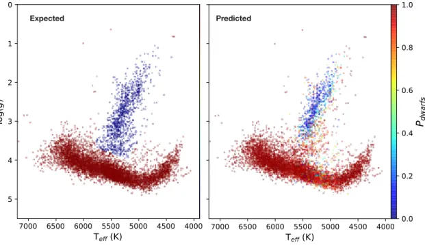
which indicates that there is no over-fitting of the data. The RFC classifies correctly the large majority of the dwarfs (96%), with less than 7% contamination by giant stars (note, that since dwarfs make up 86% of our train-ing/test set, then this implies a factor of 2 improvement over random chance). For the giants, slightly more than half are correctly classified, with relatively low contami-nation, ∼ 30%. Thus, our completeness is approximately 4 times better than “random”, and our contamination is nearly 3 times lower than “random”. Figure6 is a Kiel diagram of the expected/predicted probability for each star to be a dwarf, and we see that most of the con-tamination of the dwarfs is from sub-giants, which are preferentially classified as dwarfs instead of giants.

It is worth nothing here that, in Figure6, the surface gravity from SDSS/SEGUE decreases with the temper-ature for the main sequence stars with an effective tem-perature lower than 4,800 K. This is unexpected when compared to theoretical predictions, and it is likely a consequence of the poor determination of the surface gravity by the SSPP in this region. However this has no impact on our classification, since all the stars in this re-gion are correctly identified as dwarfs by the algorithm. The detailed performance of our classification scheme as a function of metallicity, surface gravity, effective tem-perature and (u − G)₀ color is shown in Figure 7. The completeness and contamination are mostly constant in the range of temperature and color covered by the giants. The completeness and contamination are also constant with metallicity up to [Fe/H]' −1.2, after which the completeness drops rapidly (from 70% at [Fe/H]= −1.3 to 20% at [Fe/H]= −1.0), correlated with a dramatic in-crease in the contamination. We conclude that the clas-sification works well for giants with metallicities below [Fe/H]=−1.2, but fails to identify the most metal-rich giants. There is also a drop in the completeness of the giants at a surface gravity of log(g) of 3.3, which cor-responds to the sub-giants being preferentially classified as dwarfs.

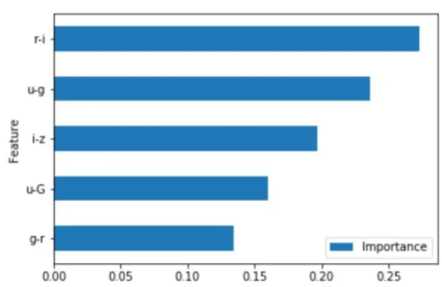
The relative importance of each photometric color in the classification scheme, computed using the feature im-portances method implemented in the sklearn package, is shown in Figure8. This method uses the weight of each feature in each node of the different trees of the RFC to measure the relative importance of such feature for the classification. The most important feature is the (r − i)0

color, with around 1/4 of the information used to clas-sify the stars coming from it. This is not surprising since this color is a good indication of the effective tempera-ture, therefore we assume that this color is being used to select the temperature ranges that preferentially con-tains giants (4, 900 ≤ Te f f ≤ 5, 500 K). The second most

Dwarfs or giants? 4000 4500 5000 5500 6000 6500 7000 7eff (.) 0 1 2 3 4 5 lo g (g ) DwDrfs GiDnts 0.0 0.2 0.4 0.6 0.8 1.0 Pdw a rf s Expected 4000 4500 5000 5500 6000 6500 7000 7eff (.) 0 1 2 3 4 5 lo g (g ) DwDrfs GiDnts 0.0 0.2 0.4 0.6 0.8 1.0 Pdw a rf s Predicted 4000 4500 5000 5500 6000 6500 7000 7eff (.) 0 1 2 3 4 5 lo g (g ) DwDrfs GiDnts 0.0 0.2 0.4 0.6 0.8 1.0 Pdw a rf s

Figure 6. Kiel diagrams where each point correspond to a star in the test set color-coded by the probability of it being a dwarf. The expected probability, or the actual class of stars, is show in the left panel and the predicted probability from our algorithm is shown in the right panel.

1.00 1.25 1.50 1.75 2.00 2.25 2.50 2.75 3.00 (u − G)0 0.0 0.2 0.4 0.6 0.8 1.0 )raFtion Completness Contamination −2.5 −2.0 −1.5 −1.0 −0.5 [FH/H] 0.0 0.2 0.4 0.6 0.8 1.0 FraFtion ComplHtnHss Contamination 1 2 3 4 5 log(g) 0.0 0.2 0.4 0.6 0.8 1.0 )raFtion Completness Contamination 4400 4600 4800 5000 5200 5400 5600 5800 Teff (.) 0.0 0.2 0.4 0.6 0.8 1.0 )raFtion Completness Contamination Completeness Contamination Completeness Contamination (a) (b) (c) (d) Completeness

Contamination Completeness Contamination

Figure 7. Completeness (blue) and contamination (orange) of stars classified as giants by the RFC in the test set as function of (a) spectroscopic metallicity, (b) surface gravity, (c) effective temperature, (d) color (u − G)₀.

Figure 8. Relative importance of each color in the classifi-cation of dwarfs and giants by the RFC.

important feature is (u − g)0, which has a tight

corre-lation with the metallicity of MSs (Ivezi´c et al. 2008;

Ibata et al. 2017b). A similar correlation exists for the giants, albeit one with a different zero point (Ibata et al. 2017b). The other colors, that account for ∼ 50% of the relative importance, presumably give additional minor complementary information (on the metallicity, temper-ature, surface gravity) to disentangle the dwarfs from the giants, using the full shape of the spectral energy distribution (SED).

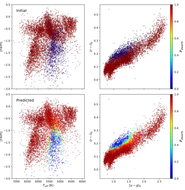
From Figure 8, we conclude that the dwarfs/giant classification primarily uses photometric features that trace temperature and metallicity. This becomes more clear in Figure9, where the locus of giants is obvious on the effective temperature-metallicity diagram (left pan-els), or on a color-color diagram using the two most important photometric features, the (r − i)0 and the

(u − g)0 colors (right panels). The two upper panels

of Figure 8 show clearly that the SDSS/SEGUE sam-ple do not contain a large number of metal-poor dwarfs in the temperature range that overlap with the ma-jority of giants (4, 900 ≤Te f f ≤ 5, 500 K). The

selec-tion criteria for SDSS/SEGUE are generally complex (Yanny et al. 2009a). However, the absence of metal-poor dwarfs is exacerbated by the relatively shallow depth of the SDSS/SEGUE dataset, that does not con-tain stars fainter than G ' 18 mag. This means dwarfs are generally quite close and so are preferentially se-lected from the disk, which is much more metal rich on average than the halo.

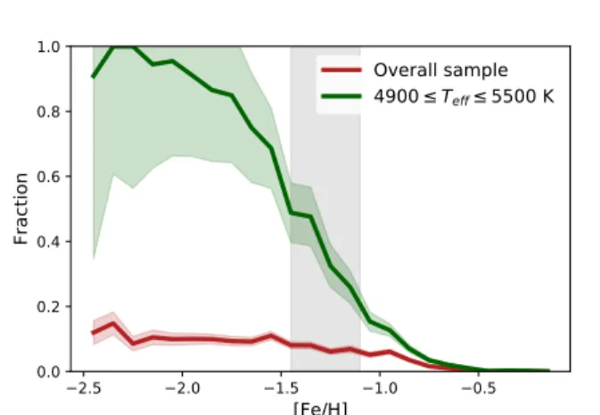
As a consequence of this, the fraction of true dwarfs misidentified as giants increases drastically with the metallicity in this temperature region, as shown in Fig-ure10. The majority of true dwarfs with [Fe/H]< −1.5

are classified as giants by the algorithm. This should be compared to the overall sample, in which the fraction of misidentified dwarfs never exceeds 0.2 (and which is al-most constant for metallicity lower than [Fe/H]= −1.0).

Intriguingly, it is fascinating to note that even in the temperature range including the giants, more than 50% of true dwarfs (and true giants) are correctly identified between −1.45 ≤[Fe/H]≤ −1.1. This demonstrates that additional features, not just those relating to temper-ature and metallicity, are been used by the algorithm to classify dwarfs and giants. It seems reasonable to suppose that these feature relate directly to the surface gravity of the stars, such as the Paschen lines presents in the i, z and G-bands or the Ca H&K absorption lines in the u, g and G-bands (seeStarkenburg et al. 2017).

Our finding partially contradicts Lenz et al. (1998), who show that it is not possible to simultaneously sep-arate cleanly stars by temperature, metallicity, and sur-face gravity using the SDSS filter set (which are broadly similar to the CFIS and PS1 filters), with the notable ex-ception of A-type stars. However, their analysis did not take into account possible non-linear relations between photometric colors and the relevant stellar parameters. By construction, our RFC accounts for non-linearity in these relations, allowing us to use photometry to better predict the probability of a star being a dwarf or a giant. We also note that we experimented with different meth-ods to classify dwarfs and giants, including ANNs and a principal component analysis (PCA). We found that the ANN gives similar results to the RFC, but the results were less easy to interpret; the PCA did not produce good results due to its requirement of linearity.

With the advent of new spectroscopic survey in the northern hemisphere, such as WEAVE and SDSS-V, the number of metal-poor dwarfs with a effective tempera-ture between 4, 900 ≤Te f f ≤ 5, 500K that have spectra

will likely increase. These future data will be excellent training sets to improve the dwarf/giant classification. Indeed, we will discuss later other issues with the train-ing/test sets for which future spectroscopic datasets will likely provide essential improvements.

It is important to keep in mind that the giant sample produced by the algorithm may contain a non negligible fraction of actual metal-poor dwarfs, since dwarfs gen-erally outnumber giants in any survey. However, in the critical temperature range (4, 900 ≤Te f f ≤ 5, 500 K), the

difference in absolute magnitude between a true dwarf and true giant at the same color is of at least ' 3 mag, equivalent to an incorrect distance of at least ' 150% (this error being even larger for redder stars). Thus, many of the misidentified dwarfs in our survey can be easily identified by consideration of their Gaia proper motions.

Dwarfs or giants? −3.0 −2.5 −2.0 −1.5 −1.0 −0.5 0.0 0.5 [Fe/H] Initial 0.0 0.1 0.2 0.3 0.4 0.5 (r − i)0 4000 4500 5000 5500 6000 6500 7000 Teff (K) −3.0 −2.5 −2.0 −1.5 −1.0 −0.5 0.0 0.5 [Fe/H] Predicted 1.0 1.5 2.0 2.5 (u − g)0 0.0 0.1 0.2 0.3 0.4 0.5 (r − i)0 0.0 0.2 0.4 0.6 0.8 1.0 Pdw a rf s 0.0 0.2 0.4 0.6 0.8 1.0 Pdw a rf s

Figure 9. The left panels show effective temperature-metallicity diagrams, and the right panels show a (u − g)0− (r −i)0diagram. The top panels show the distribution of true dwarfs (red) and giants (blue) of the test set. The lower panel show the same distributions where the stars are color-coded as a function of their probability to be dwarfs according to the algorithm.

The next step of the algorithm is to determine, inde-pendently for each of the two classes, the photometric metallicity and the absolute magnitude (and thus the distance) of each star.

There have been many studies that estimate the pho-tometric parallax of stars, especially MSs (Laird et al. 1988; Juri´c et al. 2008; Ivezi´c et al. 2008; Ibata et al. 2017b; Anders et al. 2019). This is possible because the MS locus has a well defined color-luminosity rela-tion. Using this property,Juri´c et al.(2008) derived the distances of 48 million stars present in the SDSS DR8 footprint out to distances of ∼ 20 kpc using only r and i-band photometry. However, this study did not take into account the effects of metallicity, which shifts the

luminosity for a given color, more metal rich-stars being brighter than the metal-poor ones (Laird et al. 1988, but also see Figure 3 fromGaia Collaboration et al. 2018b). Age has less impact on the photometric parallax because its effect is to depopulate the bluer stars while maintain-ing the shape of the MS locus for the redder stars.

It is well known that it is possible to derive the photo-metric metallicity of a star by measuring its UV-excess (Wallerstein & Carlson 1960;Wallerstein 1962;Sandage 1969), since metal-poor star have a stronger UV-excess than metal-rich stars. Carney (1979) shows that is is possible to measure the metallicity of a star with a pre-cision of 0.2 dex for stars with photometry better than 0.01 dex in the Johnson U BV filters. More recently

−2.5 −2.0 −1.5 −1.0 −0.5 [Fe/H] 0.0 0.2 0.4 0.6 0.8 1.0 Fraction Overall sample 4900 ≤ Teff≤ 5500 K

Figure 10. Fraction of actual dwarfs misidentified as giants as a function of metallicity, for the overall test sample (red), and for a narrower range of effective temperature between 4, 900 ≤Te f f ≤ 5, 500 K (which is the temperature range of the giants). The gray shadowed area highlights the metal-licity region where more than 50% of dwarfs and giants are correctly identified.

Ivezi´c et al. (2008) showed that it is possible to obtain a similar precision with the ugr SDSS filters, and used it to derive the photometric parallax of 2 million F/G dwarfs up to 8 kpc, where the distance threshold is lim-ited by the precision of the SDSS u-band (see alsoIbata et al. 2017b).

In this section, we build on this body of literature and present a data-driven method to estimate the metallicity and distances of dwarf stars (Section 3.3.1) and giants (Section3.3.2).

3.3.1. Dwarf stars

We first determine the photometric metallicity of the dwarfs before computing the distance of these stars. To determine the distance, we prefer to use the absolute lu-minosity derived using the Gaia parallaxes, rather than the parallaxes themselves, considering that a large num-ber of Gaia parallaxes are negative due to the stochas-ticity of the survey (Luri et al. 2018). By construction, using the absolute magnitude leads to derived distances that are always positive.

A degeneracy exists between metallicity, luminosity, and colors, especially for stars of high metallicity (Lenz et al. 1998). As pointed out byIbata et al.(2017b), ne-glecting the impact of metallicity on the derived absolute magnitude can lead to important errors, rendering the derived distances invalid. In principle, it should be pos-sible to obtain the metallicity and absolute magnitude of the dwarfs simultaneously, in a single step. However, as described below, only about half of the dwarfs that have good metallicity measurements also have good enough parallax measurements to estimate their absolute

mag-nitudes. In order to use the maximum amount of infor-mation available, we decide to use two steps, the first to determine the photometric metallicity and the second to estimate the absolute magnitude.

To evaluate the photometric metallicity of the dwarfs, we construct a set of five independent ANNs, whose inputs are the same colors used for the dwarf - giant classification. Using a set of independent ANNs rather than only one is preferable because it allows us to esti-mate the systematic errors on the predicted values gen-erated by the algorithm. Using a sub-sample of the training set, we found that 5 independants ANNs gives similar systematic errors that with 10 or 15. More-over, it also prevents any eventual over-fitting. The five ANNs, constructed using the Keras package ( Chol-let 2015), have different individual architectures and are composed of between two and five hidden layers. As for the RFC, the training set is used to find the best architecture of each ANN with a k-fold cross validation method with five sub-samples, where we impose that each ANN has an independent architecture. The pa-rameters used to train/test4 the ANNs are the adopted spectroscopic metallicities from the SSPP (FeHadop) and their uncertainties for ∼ 35, 000 dwarfs from the SDSS/SEGUE dataset. The techniques mentioned ear-lier for estimating metallicity from photometric pass-bands have typical uncertainties of δ[Fe/H]' 0.2 (rela-tive to the spectroscopic measurement). A quality cut is applied on the spectroscopic dataset to only use dwarfs with adopted uncertainities on the spectroscopic metal-licity of δ[Fe/H]s pectr o ≤ 0.2. We note that this

crite-rion has only a very small impact on the SDSS/SEGUE dwarf catalog, since it removes ∼ 100 stars.

The loss (or cost) function used to train the ANNs is a modified root mean square function which includes the uncertainties on the metallicity:

L = v t 1 n n Õ i=1 (ytr ue,i− ypr ed,i)2 δy2 i , (1)

where ytr ue,i and δyi are the spectroscopic metallicity

and its uncertainty for the ith _{star, and y}

pr ed,i is the

corresponding metallicity predicted by the algorithm. Once each ANN is trained, we define the metallicity of the dwarfs ([Fe/H]Dwar f) as the median of the outputs

of the five ANNs, and the systematic error as their stan-dard deviation. The difference between the photometric

4 As for the dwarf - giant classification, the spectroscopic dwarf dataset is split between a training and test set. However, the results shown in Figures11and 12are made with the combined dataset to improve their clarity.

Dwarfs or giants? −2 0 2 4 6 8 0G true −2 0 2 4 6 8 0G p h o to −1.5 −1.0 −0.5 0.0 0.5 1.0 1.5 0G photo-0G true 0.0 0.2 0.4 0.6 0.8 1.0 1.2 Counts σ 0.32 dex −3.0 −2.5 −2.0 −1.5 −1.0 −0.5 0.0 0.5 [FH/H]spectro −3.0 −2.5 −2.0 −1.5 −1.0 −0.5 0.0 0.5 [F H /H ]ph o to −1.0 −0.5 0.0 0.5 1.0 [FH/H]photo-[FH/H]spectro 0.0 0.5 1.0 1.5 2.0 2.5 Counts σ 0.15 dH[ −3.0 −2.5 −2.0 −1.5 −1.0 −0.5 0.0 0.5 [FH/H]Segue −1.0 −0.5 0.0 0.5 1.0 [F H /H ]Sh o to -[ FH /H ]Seg u e 0.33 0.20 0.19 0.13 0.11 −2 0 2 4 6 8 MG, Gaia −1.0 −0.5 0.0 0.5 1.0 MG , p h o to − G a ia 0.82 0.55 0.34 0.33 0.28 0.30 0.32 0.29

Dwarfs

[Fe/H]

M

G

Figure 11. Comparison of the “true” and derived metallicity for dwarfs (top panels), and the true and derived absolute magnitudes for dwarfs (bottom panels). The left panels show the true and derived quantities plotted against each other. The one-to-one relation is shown (solid lines), and the dashed and dotted lines correspond respectively to the 1-σ and 2-σ deviation. The right panels show the distribution of the differences between the true and derived quantities, with a Gaussian fit overlayed. The horizontal panels shows the residue between the quantity predicted by the algorithm and the “true” values. The lines are the same than on the left panels. The red error bars show the scatter of the derived parameters at different location.

and the spectroscopic metallicity is shown in the two up-per panels of Figure11, and isσ[F e/H]= 0.15 dex. This

is a moderate improvement on the method ofIbata et al.

(2017b) (σ[F e/H] = 0.20 dex). Note that the residuals

do not show any significant trend with the metallicity, except for the most metal-poor stars ([Fe/H] < −2) for which the photometric metallicity tend to be higher than the spectroscopic measurement. We remark that the residuals increase with decreasing metallicity, indicating that the predicted photometric metallicities are less reli-able for stars with metallicity lower than [Fe/H]< −2.0. This will be partly due to the lower number of stars present in the training set at this metallicity than at higher metallicity. The average uncertainty on the spec-troscopic metallicity of the dwarfs isδ[Fe/H]= 0.04 and the systematic error is δ[Fe/H]Dwar f ,sys = 0.02. Thus,

most of the scatter on our metallicity measurement is due to the intrinsic apparent color variation of the dwarfs of similar metallicity.

Once the metallicity is determined, it is used in com-bination with the colors to estimate the absolute magni-tude of each dwarf, and therefore its distance. As for the metallicity, a set of five ANNs is constructed, where the inputs are the same colors used previously in addition to the derived metallicity. The output is the absolute magnitude in a given band. We decide to use the Gaia G band as a reference since this is the filter with the lowest photometric uncertainty at a given magnitude.

The absolute magnitude of the dwarfs in the SDSS/SEGUE catalog are computed from Gaia parallaxes ($) accord-ing to

MGg ai a = G0+ 5 + 5 log10($/1000). (2)

It is worth noting that Gaia tends to underestimate the parallaxes and we therefore correct all parallaxes by a global offset of $0 = 0.029 mas, as suggested by

Lindegren et al.(2018). Luri et al.(2018) show that the inversion of the parallax to obtain the distance (and so the absolute magnitude), is only valid for the stars with low relative parallax uncertainties, typically $/δ$ ≥ 5 (a relative precision of ≤ 20%). In these cases, the probability distribution function (PDF) of the absolute magnitude can be approximated by a Gaussian centered on MGg ai a with a widthδMGg ai a, such that

δMGg ai a = δG +     δ$ $ ln(10)     . (3)

A quality cut is performed on the SDSS/SEGUE dwarfs to keep only those stars with a relative Gaia par-allax measurement better than 20%. With this criterion, the mean relative parallax precision of the spectroscopic dwarf sample is ∼ 10%, corresponding to an average

un-certainty on the absolute magnitude ofδM_{Gg ai a} = 0.22 mag. The spectroscopic dwarf dataset used to train/test the set of ANNs is composed of 18, 930 stars, and is a good representation of the distribution of metallicities and absolute magnitudes in the initial dataset (covering a range of metallicity of −3.0 <[Fe/H]s pectr o < 0.5 dex,

a range in absolute magnitude 3 < MG < 7.5, and ' 600

stars with [Fe/H]s pectr o < −2.0 with good parallax

pre-cision).

The set of five ANNs used to derive the absolute mag-nitude have a different structure than the set used for the estimation of the metallicity, with four or five hid-den layers and a higher number of neurons per layer than previously. However, the loss function is the same, where ytr ue,δy and ypr ed now correspond to MGg ai a,δMGg ai a

and MGpr e d, respectively. We define the predicted

abso-lute magnitude in the G-band of the dwarfs (M_{GD w ar f}) as the median of the outputs of the five ANNs, and the systematic error (δ MGD w ar f,sys) as their standard

deviation. As illustrated in the lower panels of Figure

11, the predicted absolute magnitude shows a scatter of σMG = 0.32 mag compared to the absolute magnitude

computed from the Gaia parallaxes. This corresponds to a relative precision on distance of 15%, very similar to the precision found byIvezi´c et al.(2008). It is worth noting that the scatter is almost constant over the range of absolute magnitude, except around MGg ai a ' 4.2,

where a few stars tend to have a higher predicted ab-solute magnitude than observed. These stars are proba-bly young stars (< 5 Gyr) on the main-sequence turn-off (MSTO). Since CFIS observes at high galactic latitude (|b| > 18◦ ), their number is negligible, and we expect that this under-estimation of the luminosity of younger stars should have a negligible impact on statistical stud-ies of the distance distribution.

3.3.2. Giant stars

The method to derive the metallicity and the absolute magnitude is similar for the giants as for the dwarfs, with a first set of ANNs to derive the metallicity, and second set of ANNs to estimate the absolute magnitude. The architecture of the two sets of ANNs are exactly the same as for the dwarfs.

The adopted metallicities and the uncertainties for the spectroscopic giants are used to train/test the first set of ANNs. Again, we apply a quality cut on the metallicity that uses only the 5, 670 giants with a metallicity pre-cision better thanδ[Fe/H]_{s pectr o} ≤ 0.2 (this quality cut removes less than 0.5% of the initial giant sample). The procedure used is exactly the same as for the dwarfs, and the predicted metallicity of the giants ([Fe/H]_Giant) is equal to the median of the five ANNs outputs, and

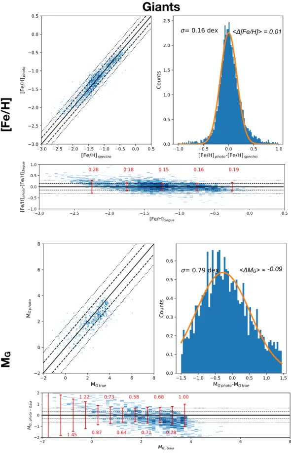
Dwarfs or giants? −3.0 −2.5 −2.0 −1.5 −1.0 −0.5 0.0 0.5 [FH/H]spectro −3.0 −2.5 −2.0 −1.5 −1.0 −0.5 0.0 0.5 [F H /H ]ph o to −1.0 −0.5 0.0 0.5 1.0 [FH/H]photo-[FH/H]spectro 0.0 0.5 1.0 1.5 2.0 2.5 Counts σ 0.16 dH[

Giants

[Fe/H]

M

the systematic errors (δ[Fe/H]Giant,sys) is the standard

deviation of these outputs. As shown on the two top panels of Figure 12, the residual between the photo-metric and spectroscopic metallicity is σ[F e/H] = 0.16

dex and does not show any trend with metallicity, ex-cept for stars with [Fe/H]<-2.0 as for the dwarfs. This is a very significant improvement over previous studies, where the giants were not treated separately from the dwarfs, leading to an overestimation of their metallicity by [Fe/H]= 0.16 dex (Ibata et al. 2017b).

In contrast to the dwarfs, it is not possible to keep only the giants with a relative Gaia parallax accuracy . 20%. At a similar luminosity, the giants are more distant than the dwarfs, which leads to a higher uncertainty in their parallax. Adopting the same selection as for the dwarfs creates a dataset of only ' 1, 000 stars, whose overall metallicity distribution is very different from the overall metallicity distribution of the giants. Indeed, the large majority of these stars (∼ 670) have a metallicity higher than [Fe/H]> −1 while 3/4 of the overall spectroscopic giants dataset has a metallicity lower than [Fe/H]< −1 with a peak around [Fe/H]' −1.4 (see the lower panel of Figure13). In addition, more than 60% of the giants with a parallax accuracy of . 20% seem to be sub-giant stars, misidentified by our dwarf - giant classifier.

About 2/3 of the spectroscopic giants have a rela-tive precision on their parallax measurement higher than 20%. Therefore, the PDF of their absolute magnitude cannot be approximated by a Gaussian, as was the case for the dwarfs. As shown by Luri et al. (2018), their PDF is asymmetric and the maximum is not centered on the “true” absolute magnitude. Using the maximum of the PDF in these cases leads to an underestimate of the distance, and therefore underestimates the absolute magnitude. Depending on the relative parallax preci-sion, the “true” absolute magnitude can be more than 1-σ away from the maximum likelihood value.

In principle, we could perform a data augmentation of the spectroscopic giants dataset to take into account the uncertainties on the different parameters, especially the parallax. This can be done by Monte-Carlo sampling the spectroscopic giants dataset in a range of 2.5 - 3 σ around the maximum likelihood of the observables. In order not to add any bias, this distribution should be symmetric around the maximum likelihood of the different parameters. However, to keep a physical value of absolute magnitude, the parallaxes should be positive. This leads to a dataset composed of stars with$ − 2.5 ∗ δ$ > 0, reducing drastically the number of stars used to train the model, which also biases the sample to much more metal-rich stars, similar to the effect of cutting on the parallax uncertainties described above.

For these reasons, we use all the spectroscopic giants that have a positive parallax measurement. Following

Hogg et al. (2018), we apply a quality selection on the parallax to keep only giants with an uncertainty on the parallax δ$ < 0.1 mas, so that we are not dominated by stars with extremely poor measurements. The final dataset used to train/test the set of ANNs is composed of 3, 497 giants. However, we found that for this giant sample, the Gaia parallaxes have to be corrected by an offset of $0 = 0.033 mas in order to obtain reasonable

distances for the globular clusters (see Section4.3). This offset is slightly higher than for the dwarfs (of$0= 0.029

mas), but lower than the offset of$0 = 0.048 mas found

byHogg et al.(2018) for red giant stars.

Due to a lack of precise parallaxes, the exact PDF (and so the uncertainties) of the absolute magnitude (calcu-lated using Equation2) cannot be known for most of the giants without adopting a prior on the density distribu-tion of the giants in the Milky Way. We cannot, there-fore, estimate the uncertainties on the absolute magni-tude using Equation3. For this reason, the loss function used as a metric for the ANNs is a standard root mean square that does not take into account the uncertainties on the absolute magnitude.

The scatter on the absolute magnitude shown in the left panel of Figure 12 is σ_MG = 0.79 dex, with a bias of ∼ −0.28 dex, similar to the median of the residuals (Me(∆MG)= −0.28). This bias is a consequence of the

underestimation of the distance to the giants using the values given by the maximum of the PDF. The mean residual is larger (< ∆MG>= −0.09), because it is

influ-enced by those stars with the largest residuals, a result of the limited statistical sample.

Indeed, the Gaia parallaxes of these stars are inaccu-rate, and distances obtained by inverting the parallax tend to underestimated the true distance of these stars (Luri et al. 2018). Thus the absolute magnitudes used to train the relation are inaccurate, and are likely un-derestimate. It is therefore not possible to use the scat-ter between the predicted absolute magnitude and the absolute magnitude obtain from the Gaia parallax to verify that the predicted distances are correct with this method. However, as we will show in Section4.3 using the globular clusters present in the CFIS footprint, the distances of the giants thus determined gives good esti-mates of their real distances, despite the lack of precision of the absolute magnitudes used to train the relation.

4. PERFORMANCE OF THE ALGORITHM 4.1. Verification from SDSS/SEGUE

We now apply the algorithm to the full SDSS/SEGUE dataset for stars with a spectroscopic SN R ≥ 25. The

Dwarfs or giants? −2.5 −2.0 −1.5 −1.0 −0.5 0.0 [Fe/H] 0 500 1000 1500 2000 2500 MDF Dwarfs True dwarfs PDwarf> 0.5 PDwarf≥ 0.7 −2.5 −2.0 −1.5 −1.0 −0.5 0.0 [Fe/H] 0 50 100 150 200 250 300 MDF Giants True giants PGiant> 0.5 PGiant≥ 0.7

Figure 13. Metallicity distribution function (MDF) of the dwarfs (upper panel) and giants (lower panel). The gray his-tograms are the spectroscopic MDFs from the SDSS/SEGUE catalog using the adopted metallicity from the SSPP. The blue and red histograms are the predicted photometric MDFs for the stars, where blue and red lines correspond to stars with a confidence of being a dwarf/giant of 0.5 and 0.7, re-spectively. The excess of dwarfs around [Fe/H]' −0.5 and the depletion of giants more metal-rich than [Fe/H]= −1.0 are the consequence of the mis-classification of actual metal-rich giants by the algorithm.

photometric metallicity distribution function (MDF) from the stars classified by the algorithm as dwarfs (PDwar f ≥ 0.5) and giants (PGiant ≥ 0.5) are

com-pared to the spectroscopic metallicity distribution of the dwarfs and giants for the SDSS/SEGUE in Figure

13.

The expected and predicted MDFs for dwarfs and gi-ants in Figure 13 are generally similar, especially for the dwarfs. For the giants, the agreement at the metal-poor end is good, but the number of giants predicted to have [Fe/H]> −1.0 falls to zero. This is a direct conse-quence of the mis-classification of the most metal-rich giants, as discussed in Section 3.2. Further, these mis-classified giants are the origin of the excess of dwarfs around [Fe/H]' −0.5 compared to the number expected from the spectroscopy.

If we consider only stars classified as dwarfs/giants with high confidence (P_{Dwar f /Giant} ≥ 0.7; red lines in

Figure13), the MDF of the dwarfs is almost unchanged. This means that the large majority of dwarfs are clas-sified by the algorithm with high confidence. For the giants, the MDF of stars classified with high confidence decreases sharply at [Fe/H]=-1.2, instead of [Fe/H]=-1.0 for the stars with PGiant ≥ 0.5. Thus, the classification

of giants is more uncertain at high metallicities than at lower metallicities. Again, this is another manifes-tation of the difficulty of the algorithm in identifying more metal-rich giants. The over-predicted number of giants around [Fe/H]=-1.8 is a consequence of the trend in the photometric metallicity relation which tends to over-estimate the metallicity of stars with [Fe/H]< −2.0, as explained in section3.3.2.

The left panel of Figure 14 compares the absolute magnitude expected using the Gaia parallaxes (MG,Gaia)

with the absolute magnitude predicted by the algorithm (MG, photo) for stars in SDSS/SEGUE with $/δ$ ≥ 5.

The stars predicted as dwarfs and giants by the algo-rithm are shown in red and blue, respectively. As ex-pected, the predicted absolute magnitude of the large majority (more than 97%) of the stars identified as dwarfs is similar to the Gaia measurements. However, a small population of dwarfs have predicted absolute magnitudes significantly lower than observed (around MG,Gaia ∼ 3). This population corresponds to

metal-rich giants/sub-giants that have been misidentified as dwarfs. For those stars identified as giants by the algo-rithm that are actually giants, the agreement between the predicted and actual magnitudes is good. How-ever, all those stars identified as giants that are actually dwarfs are estimated to be too bright.

It is not surprising, given the criterion imposed on the relative precision of the parallax, that the fraction of contaminant dwarfs is much higher than the ' 30% measured previously. Indeed, the Gaia catalog is lim-ited at a magnitude of G = 21 and since dwarfs are intrinsically less bright than giants, dwarfs in this cata-log are on average closer than giants. Since the parallax method is more precise for the stars at shorter distances, it is natural that most of the stars with relative paral-lax measurements better than 20% are actual dwarfs. Nevertheless, it is very interesting to see that the ac-tual giants have predicted magnitudes similar to Gaia’s. Moreover, the scatter is only slightly larger than for the dwarfs, despite the fact that the data used to train the set of ANNs are less accurate for giants than for dwarfs.

−2 0 2 4 6 8 0G Gaia −2 0 2 4 6 8 0G p h o to −2 0 2 4 6 8 0G Gaia −2 0 2 4 6 8 0G p h o to

Segue

Lamost

SEGUE

LAMOST

Figure 14. Distribution of the absolute magnitude computed from the Gaia parallax (x-axis) against the absolute magnitude

predicted by the algorithm (y-axis), for stars with$/δ$ ≥ 5. The left panel is for stars from SDSS/SEGUE dataset, and the

right panel is for stars from the LAMOST dataset. The stars predicted as dwarfs are in red and the stars predicted as giants are in blue. 4000 4500 5000 5500 6000 6500 7000 7eff (.) 0 1 2 3 4 5 lo g (g ) 0.0 0.2 0.4 0.6 0.8 1.0 Pdw a rf s

Figure 15. Same as Figure6but for the LAMOST dataset.

Approximately 480, 000 stars from the LAMOST DR3 catalog are present in the CFIS footprint5. While this is 10 times more than for SDSS/SEGUE, most LAMOST stars are metal-rich. Less than 3,000 LAMOST dwarfs

5 Contrary than for SDSS/SEGUE, we do not limit our analysis to stars with a higher signal-to-noise ratio.

−2.5 −2.0 −1.5 −1.0 −0.5 [FH/H] 0.0 0.2 0.4 0.6 0.8 1.0 FraFtion ComplHtnHss Contamination Completeness Contamination

Figure 16. Completeness (blue) and contamination

(or-ange) fraction of the stars from the LAMOST dataset clas-sified as giants by the algorithm as function of the spectro-scopic metallicity.

have a metallicity of [Fe/H] ≤ −1.5, and their metallicity accuracy is lower than for the corresponding metallicity range in the SDSS/SEGUE dataset. Scientifically, we are more interested in distant stars, at the faint end of the Gaia catalogue, so we focused the training of the algorithm on the SDSS/SEGUE dataset instead of the LAMOST dataset. However, this means that the LAM-OST dataset can be used to independently test and val-idate our algorithm.

Dwarfs or giants? Figure15 shows the Kiel diagram of LAMOST stars

color-coded by the probability of being a dwarf accord-ing to our algorithm. Hotter giants are generally clas-sified correctly by the algorithm, but a large number of giants are mis-classified. The completeness and contam-ination fraction of LAMOST giants is shown in Figure

16. Nearly all the mis-classified giants visible in Fig-ure 15 have [Fe/H] > −1.0, and contamination starts to increase at [Fe/H]> −1.3, demonstrating consistency with the SDSS/SEGUE sample that was used to train the algorithm.

The right panel of Figure14shows that the distribu-tion of the predicted absolute magnitude for the LAM-OST stars with$/δ$ ≥ 5 is similar to the correspond-ing distribution for the SDSS/SEGUE stars (left panel). We note that the relative fraction of actual dwarfs mis-identified as giants (bottom right corner) is smaller than for the SDSS/SEGUE dataset. This is because the LAMOST dataset is intrinsically brighter than the SDSS/SEGUE dataset. Indeed, since LAMOST stars are ∼ 2 magnitudes brighter than SDSS/SEGUE, the giants are on average closer. Thus the number of giants that have a relative parallaxes precision better than 20% is higher in the LAMOST dataset.

The number of stars present in the horizontal feature between 0 ≤ MG, Gaia ≤ 4 is higher in the LAMOST

dataset than for SDSS/SEGUE. These stars correspond to actual giants mis-classified as dwarfs. The higher number of these mis-classified stars is higher in the LAMOST dataset than in SDSS/SEGUE because the number of metal-rich giants ([FeH]>-1.0) is higher in this first one and, as mentioned earlier, the dwarfs/giants classification does not work well for these stars.

Figure 17 shows that the predicted metallicities for LAMOST stars are generally consistent with the spectroscopic metallicities obtained by the LAMOST pipeline. However, the predicted metallicity seems to be slightly under-estimated for stars with [Fe/H]≥ −0.5. Interestingly, we trace this to a systematic difference between the spectroscopic metallicity for the ∼ 4, 500 stars in common between the SDSS/SEGUE and LAM-OST datasets, as show by the red dots on the lower panel of Figure 17. Since the metallicity is calibrated on the FeHadop metallicity from SDSS/SEGUE, it is not surprising to see a similar trend in the predicted photometric metallicity.

Based on this comparison, we conclude that our method, applied to the LAMOST dataset, demonstrates the same behaviours, agreements and biases as found using the SDSS/SEGUE dataset.

4.3. Distant Galactic satellites

−3.0 −2.5 −2.0 −1.5 −1.0 −0.5 0.0 0.5 [FH/H]Lamost −3.0 −2.5 −2.0 −1.5 −1.0 −0.5 0.0 0.5 [F H /H ]ph o to −3.0 −2.5 −2.0 −1.5 −1.0 −0.5 0.0 0.5 [FH/H]Lamost −1.0 −0.5 0.0 0.5 1.0 Δ [ FH /H ] LAMOST LAMOST

Figure 17. Higher panel: Comparison of the “true” and derived metallicity for all stars in the LAMOST dataset. Lower panel: residual of the photometric metallicity against the LAMOST value in blue and in red the residual of the SDSS/SEGUE metallicity value from the SSPP against the LAMOST values. The uncertainties on the metallicity values given by LAMOST and the average residual of the photomet-ric metallcity are respectively shown by the horizontal and vertical errorbar. The dotted line shows the 1-σ of the giants (σ = 0.16) relation of the photometric metallicity determined previously.

Several Galactic satellites with known distances are included in the CFIS dataset, and present another op-portunity to independently test our algorithm. We first examine the four closest globular clusters present in the CFIS footprint, NGC 6205, NGC 6341, NGC 5272 and NGC 5466, where both dwarfs and the giants are de-tected. These are located between 7 and 16 kpc from us (see Table2).

For this analysis, we only consider stars at more than 3, 5, 2.5 and 1 half-light radius for NGC 6205, 6341,

1.00 1.25 1.50 1.75 2.00 u0− G0 −2 0 2 4 6 0G 5ef. 1.00 1.25 1.50 1.75 2.00 u0− G0 Gaia 1.00 1.25 1.50 1.75 2.00 u0− G0 PreG. 0.0 0.2 0.4 0.6 0.8 1.0 PGw a rf s 1.00 1.25 1.50 1.75 2.00 u0− G0 −2 0 2 4 6 0G 5ef. 1.00 1.25 1.50 1.75 2.00 u0− G0 Gaia 1.00 1.25 1.50 1.75 2.00 u0− G0 PreG. 0.0 0.2 0.4 0.6 0.8 1.0 PGw a rf s 1.00 1.25 1.50 1.75 2.00 u0− G0 −2 0 2 4 6 0G 5ef. 1.00 1.25 1.50 1.75 2.00 u0− G0 Gaia 1.00 1.25 1.50 1.75 2.00 u0− G0 PreG. 0.0 0.2 0.4 0.6 0.8 1.0 PGw a rf s 1.00 1.25 1.50 1.75 2.00 u0− G0 −2 0 2 4 6 0G 5ef. 1.00 1.25 1.50 1.75 2.00 u0− G0 Gaia 1.00 1.25 1.50 1.75 2.00 u0− G0 PreG. 0.0 0.2 0.4 0.6 0.8 1.0 PGw a rf s NGC 6205 NGC 6341 NGC 5272 NGC 5466

Figure 18. Color-magnitude diagrams of four globular clusters (GCs). Stars are color-coded by the probability of them being a dwarf star. The left panel shows the reference CMD of the cluster, where the absolute G−band magnitude is calculated using

the distance given in Table2. The middle panel shows the CMD whose the absolute G−band magnitude is computed using the

Gaia parallax measurement, following Equation2. The right panel shows the CMD where the absolute G−band magnitude is

calculated using our algorithm. The gray CMD in the middle and right panels is the reference CMD, and is included for easy comparison.

Dwarfs or giants?

Table 2. Predicted mean distances and metallicities for dwarfs and giants in the 4 globular clusters in Figure18as derived by

our algorithm, compared to literature values for the clusters. Literature values from: Harris(2010) (1),Deras et al.(2019) (2)

andHernitschek et al.(2019) (3)

Name D_{dwar f s} (kpc) Dgiant s (kpc) Dr e f (kpc) [Fe/H]dwar f s [Fe/H]giant s [Fe/H]r e f

NGC6205 8.1 ± 1.4 7.8 ± 1.7 7.1 ± 0.1 (2) −1.70 ± 0.3 −1.50 ± 0.16 −1.53 (1) NGC6341 8.9 ± 1.4 8.3 ± 1.1 8.3 ± 0.2 (1) −2.00 ± 0.37 −2.18 ± 0.16 −2.31 (1) NGC5272 10.2 ± 1.9 10.9 ± 2.7 10.48 ± 0.07 (3) −1.8 ± 0.37 −1.56 ± 0.18 −1.50 (1) NGC5466 14.7 ± 2.4 16.0 ± 2.5 15.76 ± 0.14 (3) −1.83 ± 0.40 −1.88 ± 0.14 −1.98 (1) −3 −2 −1 0 1 2 MG Draco dSph All δMG≤ 0.5 Pred. 1.0 1.5 2.0 2.5 3.0 u0− G0 −3 −2 −1 0 1 2 MG NGC 2419 All 1.0 1.5 2.0 2.5 3.0 u0− G0 δMG≤ 0.5 1.0 1.5 2.0 2.5 3.0 u0− G0 Pred. 0.0 0.2 0.4 0.6 0.8 1.0 Pdw a rf s 0.0 0.2 0.4 0.6 0.8 1.0 Pdw a rf s

Figure 19. Color-magnitude diagrams of the Draco dSph (top) and of NGC 2419 (bottom). The left panel shows the reference CMD of the object (using all stars in the field) where the absolute G−band magnitude is calculated using the literature distance.

The middle panels show the CMD of the stars with good precision on their intrinsic absolute magnitude (δMG≤ 0.5). The right

5272 and 5466, respectively. This removes the (sig-nificant) effect of crowding on the input photometry. We remove obvious foreground contamination by select-ing stars usselect-ing their Gaia proper motions. The abso-lute color-magnitude diagrams (CMD) of these GCs are shown in Figure18. The left panels show the CMDs us-ing the distances found in the literature (fourth column of Table2). Each star is color-coded by the probability that it is a dwarf according to our algorithm.

The color-coding in the left panels of Figure18reveals that our algorithm generally identifies the giants cor-rectly. A noticeable exception is for horizontal branch stars, which are not present in significant numbers in our training/test sets. In addition, the large majority of the dwarfs in each GC are also correctly identified. The exception to this is for the faintest stars in NGC 6205, where the fraction of dwarfs misclassified as giants increases at the faintest magnitudes. This is likely a di-rect consequence of the misidentification of metal-poor dwarfs in the temperature range occupied by giants, and discussed at length in Section 3.2.

The middle panel of Figure18show the CMDs of the clusters where the absolute G-band magnitude is com-puted directly from the Gaia parallax using Equation2. It is clear that this method is inadequate for these ob-jects, since the uncertainties on the Gaia parallaxes for stars more distant than a few kiloparsecs are generally prohibitively large. We stress that it is this fact that motivated the development of this algorithm in the first place. The right panels of Figure 18 show the CMDs where the absolute magnitude of the stars is computed via our algorithm. It is clear that the derived CMDs are much better than for the middle panels, and are rea-sonably close to the reference CMDs for each cluster. We note that the absence of any stars on the sub-giant branch in the CMDs in the right panel is a direct conse-quence of the preference of our algorithm to define those stars as dwarfs.

To verify that our algorithm predicts correct metallici-ties and distances for dwarfs and giants, we compare the mean distance and metallicity of the four GCs according to our algorithm to the value found in the literature. We select stars that have a probability to be a dwarf or a gi-ant of more than 0.7. For the dwarf samples, we require stars to have an intrinsic absolute magnitude larger than 3.7, to remove the impact of the sub-giants. The mean distances and metallicities for dwarfs and giants for each cluster are listed in Table2. For all the parameters, the derived values are within 1-σ of the literature values for the clusters.

It is important to note that the lower precision on the distance estimated for the four globular clusters by

our method is of 26% using the giants and of 18% us-ing the dwarfs, validatus-ing our method to estimate the absolute magnitude of those stars. One could notice that the mean metallicities obtained for the dwarfs for NGC 6205 and NGC 5272 are ' 0.2 − 0.25 dex lower than listed in the literature, though they are both in the 1-σ of the estimated metallicity. However, the few dwarfs of NGC 6205 present in the SDSS/SEGUE cat-alogue, have metallicities between −2 <[Fe/H]< −1.5 with a peak around 1.7. Therefore it is more likely that the under-estimation of the metallicity is related to the SDSS/SEGUE metallicity than directly related to our algorithm.

When we applied the algorithm to any stars in the field, it is not possible to remove the sub-giant contam-ination. The distances predicted by the algorithm for dwarfs in the four globular clusters without the con-straint on the intrinsic absolute magnitude of the dwarf to be larger than 3.7 are shown in Table 3. Releasing this constraint reduces systematically the predicted dis-tance of the globular clusters. However, these values are still consistent with the distance found in the literature, with the exception of NGC 5466. Due to its distance, the fraction of sub-giants/giants is larger than in the other globular clusters, leading to a more significant im-pact of these stars on the distance estimation. This bias should be considered when working with the dwarf stars at large distance (typically> 10 kpc). Interestingly, tak-ing into account the sub-giant contamination has a very little impact on the estimated metallicity, the difference with the metallicity found previously being much smaller than the scatter found with the spectroscopic measure-ment.

Table 3. Predicted mean distances and metallicity of the dwarfs in the 4 globular clusters without the constraint on the intrinsic absolute magnitude.

Name D_{dwar f s}(kpc) [Fe/H]_{dwar f s}

NGC6205 7.9 ± 1.7 −1.69 ± 0.3

NGC6341 8.5 ± 2.1 −2.0 ± 0.37

NGC5272 9.5 ± 2.2 −1.77 ± 0.36

NGC5466 11.9 ± 3.9 −1.78 ± 0.36

In addition to these relatively nearby clusters, NGC 2419 and the Draco dwarf spheroidal (dSph) are also present in the CFIS footprint. These systems are much more distant, at 79.7 ± 0.3 kpc and 74.26 ± 0.18 kpc6, respectively (Hernitschek et al. 2019). As such, only the upper portion of the giant branch in these two