HAL Id: hal-01962356
https://hal.archives-ouvertes.fr/hal-01962356
Submitted on 20 Dec 2018
HAL is a multi-disciplinary open access
archive for the deposit and dissemination of
sci-entific research documents, whether they are
pub-lished or not. The documents may come from
teaching and research institutions in France or
abroad, or from public or private research centers.
L’archive ouverte pluridisciplinaire HAL, est
destinée au dépôt et à la diffusion de documents
scientifiques de niveau recherche, publiés ou non,
émanant des établissements d’enseignement et de
recherche français ou étrangers, des laboratoires
publics ou privés.
Reconciling PC-MRI and CFD: an in-vitro study
Thomas Puiseux, Anou Sewonu, Olivier Meyrignac, Hervé Rousseau, Franck
Nicoud, Simon Mendez, Ramiro Moreno
To cite this version:
Thomas Puiseux, Anou Sewonu, Olivier Meyrignac, Hervé Rousseau, Franck Nicoud, et al..
Recon-ciling PC-MRI and CFD: an in-vitro study. NMR in Biomedicine, Wiley, 2019, �10.1002/nbm.4063�.
�hal-01962356�
DOI: xxx/xxxx
RESEARCH ARTICLE
Reconciling PC-MRI and CFD: an in-vitro study
Thomas Puiseux
1,2| Anou Sewonu
2,3| Olivier Meyrignac
3,4| Hervé Rousseau
3,4| Franck
Nicoud
1| Simon Mendez
1| Ramiro Moreno
2,31IMAG, Univ Montpellier, CNRS,
Montpellier, France
2ALARA Expertise, Strasbourg, France 3I2MC,INSERM U1048, Toulouse, France 4Department of Radiology, CHU Rangueil,
Toulouse, France
Correspondence
Ramiro Moreno, ALARA Expertise, Email: [email protected]
Present Address
IMAG, UMR 5149 CC 051, Université de Montpellier, Place Eugène Bataillon, 34095 Montpellier Cedex 5, France
Abstract
Several well-resolved 4D Flow MRI acquisitions of an idealized rigid flow phantom featuring an aneurysm, a curved channel as well as a bifurcation were performed under pulsatile regime. The resulting hemodynamics were processed to remove MRI artifacts. Subsequently, they were compared with CFD predictions computed on the same flow domain, using an in-house high-order low dissipative flow solver. Results show that reaching a good agreement is not straightforward but requires proper treat-ments of both techniques. Several sources of discrepancies are highlighted and their impact on the final correlation evaluated. While a very poor correlation (𝑟2= 0.63)
is found in the entire domain between raw MRI and CFD data, correlation as high as
𝑟2 = 0.97 is found when artifacts are removed by post-processing the MR data and
down sampling the CFD results to match the MRI spatial and temporal resolutions. This work demonstrates that, in a well-controlled environment, both PC-MRI and CFD might bring reliable and correlated flow quantities when a proper methodology to reduce the errors is followed.
KEYWORDS:
Phase Contrast Magnetic Resonance Imaging, Computational fluid Dynamics, Large Eddy simulation, cardiovascular blood flows, validation work flow.
Word count:
main text: 8972 words / references: 1373 words
1
INTRODUCTION
Hemodynamics is now recognized as a key marker in the occurrence and evolution of many cardiovascular pathologies (thrombo-sis, aneurysms, steno(thrombo-sis, aortic coarctation...). Over the last decades, time-resolved phase-contrast magnetic resonance imaging (PC-MRI)1has gained an increasing interest, giving a non-invasive and non-ionizing access to blood velocity fields in-vivo.
Nowadays, flow quantification based on 3D cine PC-MRI (or 4D Flow MRI)2emerges as a gold standard in clinical routines,
and stands out as a highly relevant tool for diagnosis, patient follow-up and research in cardiovascular diseases (CVD). Compatible with in-vivo evaluation, Computational Fluid Dynamics (CFD) is an alternative tool to provide 3D velocity fields. Although CFD accuracy depends on the model assumptions, it enables to partially bypass some experimental limitations inherent to the MRI acquisition process. Therefore, CFD coupled with MR velocity measurements has the potential to provide highly resolved blood flow insights and to grant an easy access to derived quantities such as Wall Shear Stress (WSS), pressure field, or residence time pertinent for medical diagnosis. Nevertheless, a necessary condition to consistently combine CFD predictions to MRI measurements is to ensure that both flow quantification techniques converge to the same outcome.
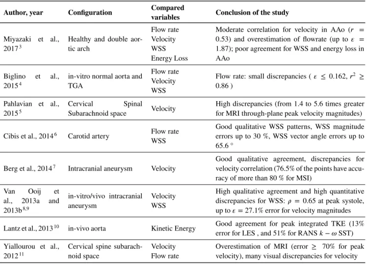
In this respect, considerable efforts have been made to compare and cross-analyse MRI measurements and CFD predictions over the last years. However, as shown in Table 1 , there is still no consensus on whether or not the two techniques lead to the same outcomes and several limitations are generally pointed out to explain the reported discrepancies.
TABLE 1 Non-exhaustive review of recent publications comparing 3D PC-MRI to CFD for Newtonian, incompressible flow in a rigid domain under pulsatile regime.
Author, year Configuration Compared
variables Conclusion of the study
Miyazaki et al., 20173
Healthy and double aor-tic arch
Flow rate Velocity WSS Energy Loss
Moderate correlation for velocity in AAo (𝑟 = 0.53) and overestimation of flowrate (up to 𝜀 = 1.87); poor agreement for WSS and energy loss in AAo
Biglino et al., 20154
in-vitro normal aorta and TGA
Flow rate Velocity WSS
Flow rate: small discrepancies ( 𝜀 ≤ 0.162, 𝑟2 ≥
0.86 ) Pahlavian et al.,
20155
Cervical Spinal
Subarachnoid space Velocity
High discrepancies (from 1.4 to 5.6 times greater for MRI through-plane peak velocity magnitudes)
Cibis et al., 20146 Carotid artery Flow rate
WSS
Good qualitative WSS patterns, WSS magnitude errors up to 30 %, WSS vector angle errors up to 65.6 °
Berg et al., 20147 Intracranial aneurysm Velocity
Good qualitative agreement, discrepancies for velocity correlation (76.5% of the points have accu-racy of more than 80 % for MSI)
Van Ooij et al., 2013a and 2013b8,9
in-vitro/vivo intracranial aneurysm
Velocity WSS
High qualitative agreement and high quantitative discrepancies for WSS: 𝜌 = 0.65 at peak systole, up to 𝜀= 27.1% error for velocity magnitudes Lantz et al., 201310 in-vivo aorta Kinetic Energy Good agreement for peak integrated TKE (13%
error for LES , and 51% for RANS 𝑘− 𝜔 SST) Yiallourou et al.,
201211
Cervical spine subarach-noid space
Velocity Flow rate
Overestimation of MRI (error ≥ 70% for peak velocity), many visual discrepancies for velocity DAo: Descending Aorta; AAo: Ascending Aorta; TKE: Turbulent Kinetic Energy; 𝑟: Pearson’s product moment coefficient; 𝜌: Spearman’s correlation coefficient; MRI-CFD error calculated as: 𝜀 = ||
|
𝑓𝐶𝐹 𝐷−𝑓𝑀 𝑅𝐼
𝑓𝑀 𝑅𝐼
|
|| where 𝑓 is the flow parameter considered. MSI stands for Magnitude Similarity Index7.
First, several acquisition parameters might limit the expected accuracy of PC-MRI measurements12. For example, a poor
spatial resolution could misrepresent the measured flow near the arterial walls (partial volume effects). Similarly, a poor temporal resolution might provide insufficient flow description, depending on its complexity and pulsatility. Time offsets between space and velocity encoding might also generate motion-induced image artifacts13. Moreover, machine-specific variability could affect
the measurements depending on both hardware and software settings14.
Regarding CFD, numerous studies highlighted the importance of imposing adequate boundary conditions15,16. Nevertheless,
as shown in Table 1 3,5,7,11, idealized velocity profiles (such as blunt, flat, or fully developed profiles) are often prescribed as
inlet boundary condition, although this may result in erroneous hemodynamic predictions15. Moreover, multiple outlets are commonplace in-vivo, from simple bifurcations (carotid artery) to entire arterial networks (pulmonary network). As a main numerical parameter driving the flow split between daughter branches, the outflow boundary condition often relies on a default
zero pressure condition17which constitutes a potential source of errors5,18. A proper way to bypass this restriction consists in
applying an outflow condition from measurements, although these latter are certainly not free of errors. For in-vitro models, an alternative way to get a flow split independent of the outlet boundary condition consists in merging the branches in a unique outlet. In this case, flow distribution within the flow domain is driven by the fluid mechanics only and a zero-pressure condition can be prescribed at the outlet. In addition, making an advised choice of CFD strategy is essential for a reliable hemodynamics prediction. As the typical Reynolds number in the (large) arteries ranges from few hundreds (laminar) to few thousands (tur-bulent), it is important to adopt a CFD strategy that accounts for the turbulence effects during the computations. However, this step is often excluded, as seen in the publications reported in Table 1 6,4. As solving the whole range of turbulence spectrum
generally requires a huge amount of computational resources, turbulence modelling strategies are often used to either partially or totally model the velocity fluctuations. Nevertheless, there are still controversies about the proper formulation to model the turbulence, and an unsuitable model could significantly affects the flow prediction10,3. Among the large number of existing
models, Reynolds Averaged Navier-Stokes (RANS) and Large Eddy Simulation (LES) are the two recurrent approaches usually adopted in flow solvers. Although more computationally demanding, Large Eddy Simulation has the advantage of capturing transition to turbulence with no changes of turbulence model parameters and can thus be considered as predictive, whereas Reynolds Averaged Navier-Stokes (RANS) models require parameters adaptations to properly represent transitional flows19,20. Recent CFD challenges also highlighted the large influence of the solver numerics and boundary conditions on the resulting flow patterns21. As demonstrated in Valen-Sendstad et al.22, the noticed divergences partially come from low-order unconditionally
stable implicit schemes proposed as default parameters by several commercial CFD codes, which generate artificial dissipation for robustness purposes.
The large variety of possible input options, from MRI setup (acquisition parameters and post-processing corrections) to the choice of CFD strategy (numerics, boundary conditions,...) or the framework of the study (in-vivo/in-vitro/in-silico), makes it difficult to draw general conclusions about the reported errors in the literature between MRI and CFD outcomes (see Table 1 ). Even in a perfect world where CFD and MRI outcomes would be virtually free of errors, the fundamental differences inherent to MRI and CFD modalities (e.g: high/low resolution in space and time, noise/noiseless data, solution in physical space/k-space filling, etc...) would most probably induce errors relative to the comparison itself. The objective of this work is then to propose a standardized procedure for comparing MRI and CFD under complex flow conditions. To establish this procedure, a preliminary step is to mitigate the sources of discrepancies coming from each of the technique in order to focus on the errors relevant to the comparison itself.
For this purpose, we designed a fully controllable, reproducible and MRI compatible experiment delivering a blood-mimicking fluid flow within a phantom which gathers topological complexities typical of that observed in-vivo. We have full control of the geometry of the non deformable flow domain and fluid rheology, thus removing classical sources of uncertainties that could be found in-vivo: segmentation errors, wall motion, blood properties. Also, although branching is present within the considered flow domain, there is only one outlet boundary so that a simple zero pressure condition can be safely prescribed. The corresponding flow is predicted by means of a high resolution LES solver, and compared with velocity fields acquired using conventional 4D PC-MRI scans at various spatial resolutions. A quantitative analysis of the differences is then performed to highlight the potential discrepancies induced by a straightforward comparison. Finally, several post-processing steps are encompassed and a generic comparison protocol is proposed to systematically correct for these sources of discrepancies.
2
MATERIAL AND METHODS
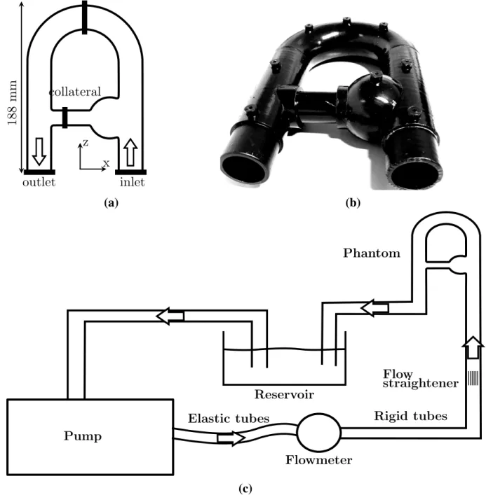
Flow phantom
The flow phantom was constructed to generate a complex and realistic flow, such as that observed in the cardiovascular system. The aim was not to reproduce a patient-specific geometry, but to gather several geometrical features yielding complex flow patterns analogous to in-vivo flow patterns, while keeping a relatively compact and well-controlled flow phantom. A 26 mm inner diameter pipe bend was designed with a 50 mm radius of curvature to mimic aortic arch blood flows. A bifurcation was set in analogy with collateral arteries. Daughter vessel sizes were designed to replicate typical flow split that can be found in-vivo between supraceliac and infrarenal arteries23. Finally, a protuberance was attached at the intersection between the collateral and
main branch, to mimic blood flows patterns in aortic aneurysms. Figure 1 b shows the final design of this MRI flow phantom. The flow in such a geometry was expected to feature complex flow structures such as flow recirculation in the aneurysm, regurgitation in the bifurcation, or a mixing layer produced by the jet at the junction of the collateral branch with the main branch.
Stereo-lithography based 3D printing technique was used to generate the flow phantom from a photopolymer resin (FormLabs Inc, Somerville, USA). Stereo-lithography is able to produce complex models with excellent surface conditions with a geometric tolerance down to 25 µm. Owing this high fidelity, we could compute the flow directly from the computer aided design (CAD) model with no surface approximations associated with a segmented geometry.
Experimental setup
The experiment was carried out using a computer controlled pump providing user-defined pulsatile flow waveforms (CardioFlow 5000 MR, Shelley Medical Imaging Technologies, London, Ontario, Canada). A blood-mimicking fluid with a kinematic viscos-ity of 𝜈= 4.02 × 10⁻⁶𝑚2∕𝑠 and a fluid density of 𝜌 = 1020 𝑘𝑔∕𝑚3was supplied to the circuit. The pulsatile flow rate delivered
by the pump was controlled by means of an ultrasonic flowmeter (UF25B100 Cynergy3 components Ltd, Wimborne, Dorset, UK), and driven to a long straight (26 mm inner diameter) rigid plastic pipe. To reduce the swirling motion of the entering fluid, a flow straightener was set upstream the tube. The flow phantom was then connected downstream. A schematic diagram of the experimental setup is shown in Figure 1 c. Inside the scanner room, the pump was positioned outside the 5 Gauss Line for MR safety considerations. Prior calibrations of the measurement devices were undertaken.
PC-MRI acquisitions
PC-MRI scans were performed on a 1.5T scanner (Siemens Magnetom Avanto, Siemens Medical Systems, Erlangen, Germany). To assess the accuracy of the inlet flow measured by MRI and to ensure that the flow was primarily axial, retrospectively gated time-resolved 2D PC-MRI measurements were acquired in the transverse plane at inlet boundary location, and compared with the reference flowmeter measurements. To increase the signal-to-noise ratio, the pixel size was set to 0.78125 x 0.78125 𝑚𝑚2
and slice thickness to 6 mm. Good agreement was found between the flowmeter and the 2D PC-MRI measurements; the mean relative error over one cycle was 𝜀2𝐷= 0.32%. It was also verified that the flow straightener disrupts any vortex coming from upstream: the in-plane velocity component measured was less than0.05𝑤, where 𝐮 = (𝑢, 𝑣, 𝑤) and 𝑤 is the through-plane velocity.
Three successive prospectively gated 4D flow MRI measurements were acquired with an isotropic voxel size of 2 mm, 3.1 mm and 3.4 mm. The flow phantom was scanned in coronal orientation with the following settings: encoding velocity VENC = 0.5 m/s in all three velocity encoding directions ; TE = 3.43-3.5 ms; temporal resolution = 49-52 ms; flip angle = 15 °. All scans were acquired without parallel imaging acceleration so that every line of the k-space was filled. A particular attention was paid to avoiding phase aliasing. To maximize SNR, the encoding velocity was set according to a numerical estimation of the maximum velocity in the flow domain.
2D cine PC-MRI inlet velocity measurements were corrected to account for partial volume effects caused by the phantom’s walls and the random noise on phase images caused by the air surrounding the phantom. A mask was applied so that all velocities at the pixels located between the wall and a user defined inner radius (𝑅𝑙𝑖𝑚 = 0.9𝑅 where 𝑅 is the radius of the circular
cross-sectional inlet surface) were corrected such that the through-plane velocity component 𝑤 at position 𝑟 equals to:
𝑤(𝑟) = 𝑤(𝑅𝑙𝑖𝑚)
𝑅− 𝑅𝑙𝑖𝑚
(𝑅 − 𝑟) (1)
As shown in Figure 2 , this near-wall mask induces a noticeable improvement of the flow waveform compared to the reference flowmeter. Quantitatively, mean relative error is reduced from 0.32% to 0.15% for 2D PC-MRI scans with respect to the reference flowmeter. For 4D Flow acquisitions with 2 mm, 3.1 mm and 3.4 mm voxel size, mean relative errors are 3.8/1.2%, 5.7/1.8% and 9.5/3.7%, respectively, for raw/masked data. As expected and mainly at peak systole, best corrections were obtained for the largest voxel size since partial volume effects are more important.
MRI Dataset processing
Velocity mapping from DICOM phase images was performed using an in-house Matlab program (The MathWorks, Natick, USA), and processings were implemented through custom VTK-based Python programs (Visualisation ToolKit, Kitware, Inc, Clifton Park, NY).
Several phase-offset corrections were applied to the raw MRI dataset. Noise in the phase images caused by the air surrounding the flow phantom was removed by thresholding the time-course standard deviation of the velocity field. Static regions were
bend
inlet
collateral
outlet
188
m
m
x
z
(a)
(b)
Reservoir
Pump
Flowmeter
Phantom
Flow
straightener
Elastic tubes
Rigid tubes
(c)
FIGURE 1 (a) Flow phantom schematic representation in the coronal plane annotated with locations of surfaces of interest. (b) 3D printed flow phantom. (c) Schematic diagram of the experimental setup.
then extracted by thresholding the signal magnitude to remove blood flow regions. Slice-wise 2D least squares second-order polynomial fit of the remaining static velocity map was performed and propagated on the entire image as a global indicator of velocity offset. Each resulting offset velocity surface was finally subtracted to the raw phase image to correct for eddy current effects24. The procedure was repeated for each phase in the cycle. Gradient field inhomogeneities were also corrected during
reconstruction of the MRI dataset. Moreover, as the blood-mimicking fluid is incompressible, the measured velocity field was corrected to meet the divergence-free condition by projection onto the space of divergence-free fields using a fractional step algorithm25,26.
0
0.2
0.4
0.6
0.8
1
0
50
100
150
t (s)
Fl
ow
ra
te
(m
l/
s)
2D cine (0.78 mm) 4D (2 mm) 4D (3.1 mm) 4D (3.4 mm)(a)
0
0.2
0.4
0.6
0.8
1
0
50
100
150
t (s)
(b)
FIGURE 2 Inlet flow waveforms over one cycle measured at different isotropic voxel sizes (a) without and (b) with near-wall velocity masking.
Computations
Blood flow motion is governed by the incompressible Navier-Stokes equations (NSE):
∇ ⋅ 𝐮 = 0 (2)
𝜌( 𝜕𝐮
𝜕𝑡 + 𝐮 ⋅ ∇𝐮
)
= −∇𝑝 + 𝜇∇2𝐮 (3)
where 𝐮, 𝑝, 𝜌 and 𝜈 are the velocity field, pressure field, density and dynamic viscosity of the fluid, respectively.
Equations 2 and 3 were discretized and solved on an unstructured tetrahedral mesh generated with GAMBIT 2.4.6 (ANSYS, Inc., Canonsburg, PA), using the YALES2BIO solver27, an in-house CFD tool designed to perform numerical simulations of blood flows in complex geometries. The YALES2BIO solver uses a finite-volume method and high-order non-dissipative numerical schemes to solve the full NSE on unstructured meshes28. So far, the solver has been thoroughly validated for both
microscopic29,30and macroscopic scales21,31,32,33biomedical applications.
Note that all the simulations were performed on two nodes (Dell PowerEdge C6320) of 28 cores Intel Xeon E5-2690 V4 2,6 GHz with 128 Go random-access memory per node.
Numerical setup
The blood-mimicking fluid was modelled as an incompressible Newtonian fluid of kinematic viscosity 𝜈 = 4.02 × 10⁻⁶𝑚2∕𝑠. A
centred fourth-order numerical scheme with an explicit fourth-order Runge-Kutta time advancement scheme was used to solve Equation 3. The time step was computed in order to ensure that the CFL number remains equal to 0.9 for numerical stability. The pressure advancement and divergence-free condition were met thanks to a fractional step algorithm25, a modified version
of the Chorin’s algorithm34. A Deflated Preconditioned Conjugate Gradient algorithm was used to solve the associated Poisson
equation35. The Sigma eddy-viscosity-based LES model36 was used to account for turbulence effects. As mentioned in the
Introduction, several reasons motivated the use of LES rather than RANS modelling strategy to account for the turbulence effects in the YALES2BIO solver. In LES strategy, the largest turbulent scales are explicitly resolved as a solution of the low-pass filtered Navier-Stokes equations while the subgrid scales are modelled. In RANS approaches, all the scales are averaged and the entire turbulence spectrum is modelled. According to the Kolomogorov’s theory (1941)37, the statistics of the smallest structures are
universal and only depend on the rate of kinetic energy dissipation and the viscosity of the fluid. On the contrary, large scales fluctuations are geometry-dependant and their shape is less generic. As it generally harbours many large scale fluctuations and
due to the complex geometries within the cardiovascular systems32, LES strategy seems then more adapted to solve this type of
flows.
A convective outlet boundary condition was imposed such that:
𝜕𝐮 𝜕𝑡 + 𝑈
𝑐𝑜𝑛𝑣𝜕𝐮
𝜕𝐧 = 0 (4)
where 𝐧 is the outward normal to the outlet surface, and 𝑈𝑐𝑜𝑛𝑣the convective velocity adjusted in such a way that it meets the
global mass conservation of the entire flow domain. All the walls were assumed rigid, consistently with the material selected for manufacturing the phantom, and no-slip boundary condition was prescribed.
A pixel-based inflow was derived from 2D cine PC-MRI measurements acquired at the inlet surface of the flow domain (see section 2). First, a 2D bilinear interpolation of the measured 2D PC-MRI velocity field was performed on the corresponding inlet surface of the CFD domain, for each of the 32 frames in the cycle. By applying at each node a discrete Fourier transform on the discrete temporal evolution of the velocity signal, a list of 17 non-redundant complex Fourier coefficients were extracted. Then, the corresponding continuous inlet velocity signal was retrieved by injecting back the Fourier coefficients in a Fourier series expansion, again computed for each node of the inlet surface.
The peak systolic Reynolds number was estimated as 𝑅𝑒 = 2𝑢𝑏𝑢𝑙𝑘𝑅
𝜈 = 1830 where 𝑅 is the radius of the principal duct and
𝑢𝑏𝑢𝑙𝑘 the averaged inlet velocity. Likewise, the Womersley number characterizing the pulsatility of the flow was defined as
𝛼= 𝑅√𝜔
𝜈 = 16.4, where 𝜔 =
2𝜋
𝑇 .
Phase-averaging CFD
During a conventional PC-MRI scan, k-space is progressively filled over hundreds of cycles and pulse sequences are often repeated to increase contrast. For this reason, confronting MRI measurements with instantaneous CFD velocity fields might not be relevant. Moreover, cycle-to-cycle fluctuations may appear for such high Reynolds number unsteady flows32. Hence, a proper
way to analyse the computed flow is to phase-average the flow velocity over a sufficiently representative amount of cycles32.
The phase averaged velocity 𝑢(𝐱, 𝑡) at spatial coordinates 𝐱 = (𝑥, 𝑦, 𝑧) and at time 𝑡 was defined as:
𝐮(𝐱, 𝑡) = 1
𝑁
𝑁∑−1
𝑘=0
𝐮(𝐱, 𝑡 + 𝑘𝑇 ) (5)
where 𝐮(𝐱, 𝑡) refers to instantaneous velocity vector and 𝑁 = 30 the total number of cycles of period 𝑇 .
Down sampling CFD
Two classical methods may be adopted for comparing CFD to MRI velocity fields on identical grids: the MRI velocity fields might be interpolated on the high resolution CFD grid (termed as HR-CFD), or HR-CFD velocities at nodes localized within a given MRI voxel might be averaged to obtain the corresponding down sampled CFD velocity value, noted low resolution CFD (LR-CFD)6. Down sampling process was achieved by linear interpolation of the CFD velocity data on a MRI sub grid where
each MRI voxel contained 216 isotropic subvoxels. The resulting down sampled velocity at each MRI voxel was then calculated as an average of the 216 sub sampled velocities.
Comparison of the results
A rigid registration between the MRI dataset and flow phantom CAD model was computed by means of a semi-automatic Iterative Closest Point algorithm38 implemented with VTK. The resulting MRI and CFD velocity maps were qualitatively
compared at several phases during the cycle. Moreover, statistical analyses of the differences observed between by MRI and CFD were computed at peak systole and based on the entire flow domain. Peak systole phase was selected because relative differences between MRI and CFD are highest at this particular phase, as also noted by Berg et al.7. All the analyses were performed with
Python using the statistical package implemented in the Scipy libraries, and were statistically significant (𝑝 <10−7). Pearson’s
0
10
20
30
40
50
60
0.6
0.8
1
Number of cycles
r
2
r
2
(kuk)
r
2
(u)
r
2
(v)
r
2
(w)
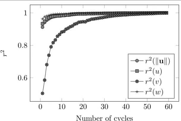
FIGURE 3 Evolution of the Pearson’s correlations (𝑟2) between phase-averaged CFD velocity computed over different numbers
of cycles the and 60-cycle phase-averaged CFD velocity. The correlations are performed on each node of the domain.
3
RESULTS
Convergence of the results
A averaging sensitivity analysis was performed to estimate the minimum amount of cycles required to converge the phase-averaged CFD velocity field. Beforehand, the first 10 cycles were removed to cancel the effect of the arbitrarily selected initial condition. The results presented in Figure 3 show that the main components of the velocity (𝑢 and 𝑤) are well-converged after few cycles (about 5 cycles) while the transverse component of the velocity (𝑣) requires more (about 30 cycles). Note that since the transverse velocity correlation is expected to be zero by symmetry, it is mostly representative of the velocity fluctuations induced by turbulence, thus the slower convergence observed in Figure 3 . Among the 60 simulated cycles, velocity field was phase-averaged over 30 cycles which was deemed sufficient for 𝑣 to reach a reasonable asymptotic value. The reproducibility of the phase-averaging process was tested by extracting and independently phase-averaging two subsequent set of 30 cycles from the 60 cycles simulated. High correlation levels were found (𝑟2(𝑢) = 0.995, 𝑟2(𝑣) = 0.930, 𝑟2(𝑤) = 0.999 and 𝑟2(‖𝐮‖) = 0.997),
showing that the outcome of the phase-averaging process does not depend on the set of cycles selected. Therefore, all the velocity fields used in this paper were averaged over 30 cycles; moreover, velocity fluctuations were calculated based on the following relation:
𝐮𝑟𝑚𝑠(𝐱, 𝑡) =
√
𝐮2(𝐱, 𝑡) − 𝐮2(𝐱, 𝑡) (6)
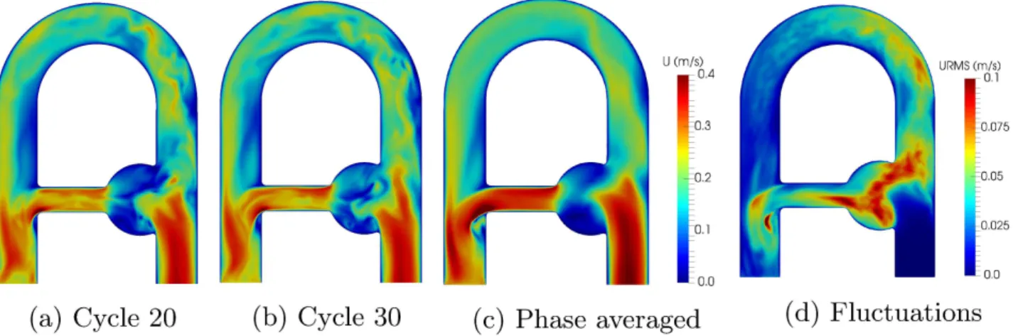
where 𝐮𝑟𝑚𝑠 stands for root-mean-square velocity. The resulting velocity fields are presented in Figure 4 . A mesh sensitivity analysis was performed to ensure the spatial convergence of the computations. Results are reported in Table 2 . The phase-averaged velocity magnitude in the aneurysmal sac results in a numerical uncertainty of1.88% for the fine mesh, with an apparent spatial order of convergence 𝑝 = 2.0 (see Sigüenza et al.39 for details). Therefore, the fine mesh was considered fine enough
for the solution to be spatially converged and independent of the spatial resolution. Moreover, the LES resolution was also investigated by evaluating the turbulent viscosity ratio 𝜈𝑠𝑔𝑠∕𝜈 where 𝜈𝑠𝑔𝑠is the subgrid scale viscosity added by the model. As
FIGURE 4 Magnitude velocity fields in the flow phantom at peak systole for cycle 20 (a), cycle 30 (b), phase-averaged (c). The velocity fluctuations (d) are expressed through 𝐮𝑟𝑚𝑠. Important cycle-to-cycle fluctuations between the instantaneous fields
indicate non reproducible disturbed zones, where turbulence is more likely to appear, while the phase averaged field encompasses dominant flow patterns.
Grid ℎ(mm) Cells×103
Coarse 1.3 622 Medium 1.0 1 284
Fine 0.7 3 812
TABLE 2 Properties of meshes used for the sensitivity analysis, as reported in Celik et al.40. ℎ corresponds to the representative
cell size.
Qualitative comparison
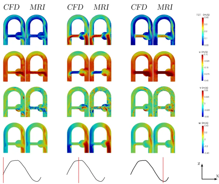
Phase averaged HR-CFD velocity fields are qualitatively compared with MRI velocity data obtained from the 2 mm voxel size with corrected phase offsets (i.e: noise masking and eddy currents) in the in-plane direction (foot-head and right-left) at several phases of the cycle in Figure 5 . Magnitude velocity maps reveal excellent agreements and show highly similar velocity patterns even in complex flow regions, such as in the aneurysm. For instance, both MRI and CFD capture the small separation region in the main branch at early systole (Figure 5 a), as well as the recirculation in the aneurysm or the back flow in the bifurcation at late diastole (Figure 5 c).
Through-plane (antero-posterior) velocity comparison shows larger visual discrepancies (Figure 5 g-i), which was expected given the low signal amplitudes (𝑣∈ [−0.05, 0.05] cm/s) with respect to the VENC (50 cm/s).
In addition, the length of the jet issued from the collateral segment appears smaller in the MRI at peak systole. In this region, the MRI does not seem to capture the mixing layer as well as CFD does. A possible explanation is that in conventional PC-MRI all three velocity components are sequentially acquired. Hence, the resulting velocity field could present noticeable temporal delay between two velocity components13. Therefore, high velocity-displacement artifacts may be observed in regions of high
convective acceleration. In practice, for the 2 mm voxel-size acquisition, a time delay of 12.5 ms was measured between 𝑢 and
𝑤. This corresponds to the time needed for a flow structure in the jet issued by the collateral to travel through approximately 2 voxels at 0.3 m/s. Note that the diameter of the collateral branch contains 8 voxels. Generally speaking, discrepancies are mainly observed in regions where the velocity fluctuations are prominent (Figure 4 ). An explanation is that eddies smaller than the voxel size should produce intravoxel phase dispersion due to the summation of the phases induced by spins with very different velocity vector directions within a voxel41.
FIGURE 5 Comparison in the coronal plane of CFD velocity fields with MRI measurements at 2 mm resolution at different instants of the cycle. First row represents the velocity magnitude, while second, third and last rows depict right-left (𝑢), up-down (𝑣) and foot-head (𝑤) velocity components respectively.
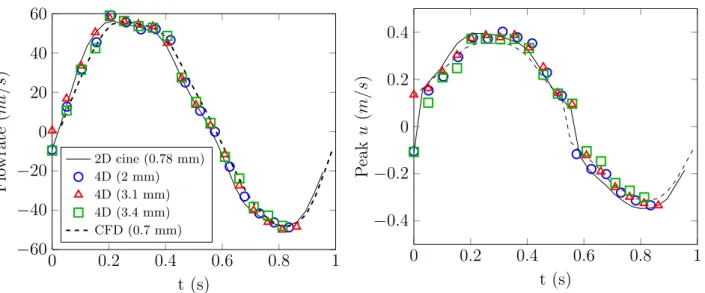
Time evolution and flow profiles comparisons
Figure 6 compares the temporal evolution of flow rate and peak velocity in the collateral segment measured by MRI for different spatial resolution with CFD predictions. Excellent agreement is found for both the flow rate and the peak velocity evolution between CFD, 2D PC-MRI and 4D Flow MRI, regardless of the spatial resolution.
The situation is not as favourable when considering velocity profiles as done in Figure 7 . Results indicate that PC-MRI velocity tends to underestimate the HR-CFD profile mainly where high velocity gradients occur. On the contrary, results reveal a good agreement in the regions where velocity gradients are small. In addition, down sampling CFD to PC-MRI spatial resolution mimics the intravoxel spin velocity averaging process inherent to PC-MRI and results in a better agreement. Note that the MRI dataset without near-wall velocity masking was willingly presented here to highlight the significant discrepancies obtained close to the walls due to partial volume effects. As an illustration, the mean relative error spans from 𝜀= 17.3% without to 𝜀 = 14.4% with near-wall velocity masking.
0
0.2
0.4
0.6
0.8
1
−60
−40
−20
0
20
40
60
t (s)
Fl
ow
ra
te
(m
l/
s)
2D cine (0.78 mm) 4D (2 mm) 4D (3.1 mm) 4D (3.4 mm) CFD (0.7 mm)0
0.2
0.4
0.6
0.8
1
−0.4
−0.2
0
0.2
0.4
t (s)
P
ea
k
u
(m
/s
)
FIGURE 6 leftFlowrate and right peak axial velocity evolution over one cycle in the collateral branch (see Figure 1 a).
FIGURE 7 Axial velocity profiles in the middle of the bend (see Figure 1 a) along 𝑦 (right-left) and 𝑧 (foot-head) axis; (— ) HR-CFD. Grey filled bar chart LR-CFD; 1st/2nd/3rd columns: 2 mm/3.1 mm/3.4 mm voxel size 4D Flow MRI acquisitions respectively. Error bars correspond to 𝑢± 𝑢𝑟𝑚𝑠
Quantitative comparison
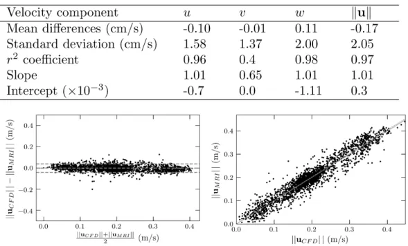
A statistical analysis of the velocity differences observed between LR-CFD and 4D Flow MRI (2 mm voxel size) at peak sys-tole is presented in Figure 8 . An excellent correlation was found for the main velocity component along z-axis. As observed qualitatively in the previous section, the in-plane velocity components (𝑢 and 𝑤) yield better correlations than the through-plane component (𝑣).
FIGURE 8 TopPearson’s product moment correlation analysis for each velocity component on the entire domain at peak systole between LR-CFD and PC-MRI measurements (2 mm voxel size). Bottom Corresponding Bland-Altman and linear regression charts of the peak magnitude velocity. Note that for clarity, only 1 over 10 data point randomly selected were plotted. Middle grey line on the Bland-Altman chart stands for mean difference ‖𝐮𝐶𝐹 𝐷‖ − ‖𝐮𝑀 𝑅𝐼‖, surrounded by its 95% confidence interval
grey lines (±2𝜎 where 𝜎 is the standard deviation). The resulting linear regression is shown in the bottom right figure with a grey dashed line, while the solid line denotes the ideal regression line.
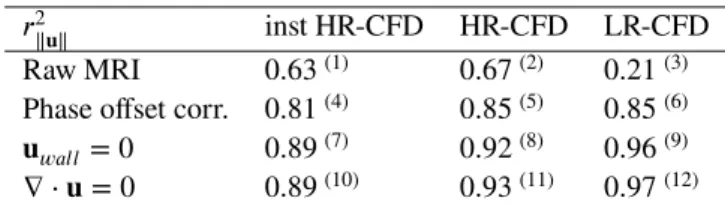
Influence of the processing on the correlation
To better understand the impact and influence of each processing step on the final comparison, statistical analyses were performed for various processing levels as defined in Table 3 . Note that only the velocity magnitude correlation results are reported, as a global indicator of the three velocity components.
The first striking result is the low correlation between raw MRI data and the instantaneous high-resolution CFD results (case 1). Note that the 63% correlation was obtained by imposing the measured velocity profile at the inlet of the computational domain as obtained by 2D cine PC-MRI. However, an approach often adopted in the literature consists in applying an idealized velocity profile (flat or parabolic) with the same integral as the actual measured profile. This approach was tested and resulted in even worse correlations, with only 𝑟2= 0.58. Results in Table 3 also show that main correlation improvements are obtained either
by down sampling the phase-averaged CFD field or by correcting for the phase offset artifacts (i.e: noise masking and eddy currents). Note that the low correlation between raw MRI and the LR-CFD is mainly due to the impact of the noise surrounding the flow phantom in the MRI measurements and affecting the points located on the wall surface. In LR-CFD, about 35% of the points are located on the surface (only 13% in HR-CFD). The noise is then masked between case 3 and 6, producing a significant improvement of the correlations. Finally, the range of variations of the correlation coefficient over the last row of Table 3 (0.89-0.97) shows the importance of degrading the CFD prediction to match the MRI spatial resolution and temporal sampling. The gain obtained by degrading the CFD data is not negligible, yet smaller, compared to the improvement generated by processing, denoising and correcting the raw MRI data (which improves the correlation from 63 % to 89 %, see first column of Table 3 ).
Reconstruction of derived quantities
The impact of the down sampling on the correlation is investigated for flow split and wall shear stress (WSS) which are flow quantities that are often regarded as biomarkers of CVD such as aortic diseases, aneurysm, congenital heart diseases, or valve regurgitation. In particular, WSS plays an important role in both aneursym initiation, growth and rupture, since changes in
𝑟2
‖𝐮‖ inst HR-CFD HR-CFD LR-CFD
Raw MRI 0.63(1) 0.67(2) 0.21(3)
Phase offset corr. 0.81(4) 0.85(5) 0.85(6)
𝐮
𝑤𝑎𝑙𝑙= 0 0.89(7) 0.92(8) 0.96(9)
∇ ⋅ 𝐮 = 0 0.89(10) 0.93(11) 0.97(12)
TABLE 3 Evolution of Pearson’s product moment correlation (𝑟2
‖𝐮‖) for the velocity magnitude at peak systole, as a function of
the level of post-processing. "inst HR-CFD" stands for the instantaneous high resolution CFD velocity field of the 30th computed cycle. "HR-CFD" corresponds to the phase-averaged CFD field and "LR-CFD" to the phase-averaged velocity down sampled to the MRI spatial resolution. "Phase offset corr." corresponds to the raw MRI dataset corrected from eddy currents and noise artifacts. "𝐮𝑤𝑎𝑙𝑙 = 0" refers to the corrected MRI dataset where a no-slip boundary condition is applied at walls and "∇ ⋅ 𝐮 = 0"
reefers to the resulting MRI velocity field modified to meet the divergence-free condition. Each comparison case is denoted with a superscript number between brackets to ease the discussion.
HR-CFD LR-CFD PC-MRI Flow split 0.39 0.41 0.44 𝑊 𝑆𝑆(Pa) 1.10 0.39 0.37 𝑟2𝑊 𝑆𝑆 0.48 0.66 1.00 𝑟2 𝑊 𝑆𝑆(𝐮𝑤𝑎𝑙𝑙= 0) 0.68 0.84 0.64
TABLE 4 Peak systolic flow split and averaged Wall Shear Stress (𝑊 𝑆𝑆) for HR-CFD, LR-CFD and PC-MRI measurements on first and second row, respectively. Flow split is defined as the collateral flow rate divided by the inlet flow rate. 𝑊 𝑆𝑆 is the WSS averaged over the entire collateral surface. The third and fourth rows correspond to the WSS correlation with respect to PC-MRI without and with zero velocity imposed at boundary walls, respectively.
WSS influence endothelial cell function and thus, promote vascular remodelling and vessel dilatation42. However,
reconstruct-ing WSS from MRI measurements is challengreconstruct-ing, especially in cardiovascular regimes where high near-wall velocity gradients occur. Moreover, the accuracy which can be expected when reconstructing WSS from MRI dataset highly depends on both wall delineation and spatial resolution9,43. In practice, existing methods to estimate wall positioning and inward normal orientation
often imply uncertainties that could cause large WSS errors9. To estimate the influence of down sampling and boundary
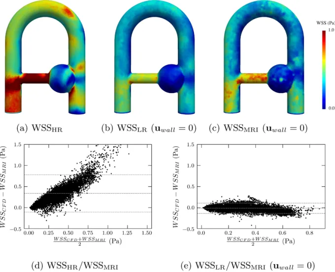
condi-tions on its reconstruction, WSS was computed from LR-CFD (WSSLR) and HR-CFD (WSSHR) velocity fields, and compared with MRI-based WSS (WSSMRI). Note that WSSMRI was computed from the MRI velocity field corrected from phase-offset artifacts (2nd row in Table 3 ). As this idealized set up provides the true position of the boundary walls, WSSLRand WSSMRI were computed after linear interpolation of the velocity data on the same low resolution mesh. A quantitative comparison of the peak systolic flow split and WSS averaged along the collateral branch as well as the WSS correlations resulting from a statisti-cal analysis on the entire wall surface are presented in Table 4 . Additionally, the WSS maps and Bland-Altman plots at peak systole are presented in Figure 9 .
As expected, regarding the flow split and the averaged WSS in Table 4 , PC-MRI measurements better match the LR-CFD than the HR-CFD. WSS sensitivity to spatial resolution and wall position induces higher relative discrepancies than for the flow split, which can be estimated with a reasonable accuracy irrespective of the spatial resolution. Moreover, down sampling and applying a no-slip boundary condition improve the agreement.
Nevertheless, the WSS correlations are generally lower than the corresponding velocity correlations. This larger discrepancy could be explained by both the loss of information associated with the down sampling process and by the sensitivity of the WSS computation to the residual noise in the near-wall voxels. To highlight the impact of the down-sampling on the correlation, WSSLRand WSSHRwere compared, with 𝑟2 = 0.69 without and 𝑟2 = 0.81 with the 𝐮
𝑤𝑎𝑙𝑙 = 0 correction. The analysis thus
shows that intravoxel averaging significantly degrades the accuracy of the gradient computation and is partly responsible for the poor WSS correlations observed between HR-CFD and MRI in Table 4 .
At last, as illustrated by the Bland-Altman plots in Figure 9 , WSSMRIlargely underestimates WSSHR. This was expected since HR-CFD being better resolved in space than MRI, it can represent larger velocity values in the wall vicinity. In other
FIGURE 9 Wall Shear Stress maps on boundary walls at peak systole. (a) WSS calculated from the HR CFD velocity field, (b) from the LR CFD velocity field (with zero velocity imposed on boundary walls) and (c) from the PC-MRI velocity field (with zero velocity imposed on boundary walls). Bland-Altman plots of the comparison between (d) WSSHRand WSSMRI(corresponding to 𝑟2
𝑊 𝑆𝑆 = 0.48 in Table 4 ) and (e) WSSLRand WSSMRIcorresponding to 𝑟2𝑊 𝑆𝑆(𝐮𝑤𝑎𝑙𝑙= 0) = 0.84 in Table 4 .
words, the voxel averaging performed through the MRI acquisition smoothens the (strong) velocity gradients present in the wall region. Degrading the CFD results allows a much better comparison as shown in Figure 9 .
4
DISCUSSION
This study proposes a methodology for correcting the discrepancies that arise when comparing MRI to CFD in complex flow conditions. The results obtained for the idealized flow clearly highlight that some discrepancies remain even after errors asso-ciated with boundary conditions, numerics, or turbulence modeling are minimized in the CFD part. Indeed, we noted that a straightforward comparison of the two modalities only produces a very poor agreement (𝑟2
|𝐮‖= 0.63). Some post-processing
cor-rections were thus proposed, that drastically increased the velocity correlations (𝑟2|𝐮‖= 0.97). To this respect, post-processing of PC-MRI dataset such as correcting phase-offset errors and near-wall velocity masking produces a more realistic output and better matches with the CFD outcome. Moreover, forcing the flow to meet the incompressibility constraint and imposing a zero velocity at the boundary walls is an efficient way of correcting the non-physical noise present in the measurement. As for imaging data post-processing, some CFD degradations are required to match the MRI spatio-temporal resolution, and therefore improve the correlation. Phase-averaging of velocity fields produces a mean representation of the flow which is suitable to match the
MRI data acquisition process. Down sampling CFD velocity fields allows to mimic the acquisition of PC-MRI signal, and leads to a coherent comparison.
Two hemodynamic biomarkers (WSS and flow split) derived from the velocity field were also investigated in this work and resulted in significant differences of sensitivity to the input velocity field. Being an integrated quantity, the flow split is very little sensitive to local errors such as the near-wall noise. On the contrary, WSS highly depends on the wall delineation and the nearby velocity measurements. Results showed that enforcing a zero velocity at boundary walls seems adapted for computing the velocity gradient and that the latter is also very sensitive to the spatial resolution.
Nevertheless, several discrepancies were not corrected, and some limitations of the study remain. Poor correlations due to a low Velocity-to-Noise ratio (VNR) in the y-component of the velocity 𝑣 were noticed. This may be bypassed by using multiple VENC based on several flow acquisitions with phase wraps correction using phase unwrapping44. Using MRI, the different axes
velocity components are sequentially acquired Because of the sequential measurement by MRI of the different velocity compo-nents, interleaved velocity encoding might involve non-negligible time shifts between two components of the velocity, mainly in regions with disturbances. Reducing the echo time decreases this delay and thus mitigates the blur in phase image. Another possibility is to use non interleaved velocity encoding sequences45. It was also observed that the largest velocity differences are
mainly located where CFD yields fluctuating velocities. As already discussed, this could be explained by the signal loss due to intravoxel dephasing. In order to quantify these remaining divergences, one could estimate the amount of PC-MRI subvoxel velocity fluctuations by deriving the intravoxel velocity standard deviation from two signal measurements with different first moment gradients46. Additionally, partial k-space filling or parallel imaging such as GRAPPA or SENSE technologies should
reduce the acquisition time, while decreasing the SNR. To improve the agreement, one could also take part of the phase images noise into account by considering the theoretical Rician distribution of the noise in the CFD velocity field47. Regarding the
WSS, a wall law that would give a continuous representation of the near-wall velocity profile could yield better results. Advanced interpolation techniques (such as B-spline or polynomial) to model the near-wall velocity spatial evolution have already been employed in the literature and resulted in better WSS estimates43.
As the present analysis was limited to in-vitro idealized flow conditions, several in-vivo features were not discussed and would certainly produce very different outcomes. For example, considering non-rigid walls would either require a dynamic assessment of the wall position during the cardiac cycle or an a priori knowledge of the mechanical properties of the walls to account for the fluid-structure interaction in the simulations. The velocity patterns should be significantly affected and both the velocity and WSS errors would certainly increase. Although the blood-mimicking fluid used in the experiment is Newtonian, modeling blood rheology under in vivo conditions is still very challenging.
In conclusion, the present study has proposed a proof of concept workflow for mutual validation of MRI and CFD under well controlled and idealized conditions. The main aim of this study was to show that in a well-controlled environment with suitable prior processing, both MRI measurements and CFD predictions bring trustworthy and equivalent global flow quantities. This framework might further be used to estimate the level of confidence that the MRI signal can guarantee as a function of the MRI input settings. For instance, if the MRI signal agrees locally well with HR-CFD, one could assume that some flow-sensitive hemodynamic variables such as WSS might guarantee reasonable estimates. On the contrary, a MRI signal providing only global flow information might be reliable in terms of flow split but not for direct estimation of WSS. More generally, this work addresses the question of the accuracy which can be expected in clinical routine when using time-restraint low-resolution MRI protocols to assess an hemodynamic outcome.
ACKNOWLEDGMENTS
The authors would like to thank Dr. Moureau and Dr. Lartigue (CORIA, UMR 6614) and the SUCCESS scientific group for providing the YALES2 code, which served as a basis for the development of YALES2BIO. Centre Pro3D and Yvan Duhamel are acknowledged for providing access to 3D printing facilities and time allocated to construct the MRI phantom. Simulations were performed using HPC resources from GENCI-CINES (Grant 2016-c2016037194) and with the support of the High Perfor-mance Computing Platform MESO@LR, financed by the Occitanie / Pyrénées-Méditerranée Region, Montpellier Mediterranean Metropole and the University of Montpellier. We finally would like to thank the LabEx Numev (convention ANR-10- LABX-20).
Financial disclosure
None reported.
Conflict of interest
The authors declare no potential conflict of interests.
References
1. Moran P. R.. A flow velocity Zeugmatographic interlace for NMR imaging in humans. Magnetic Resonance Imaging. 1982;1:197-203.
2. Markl M., Chan F. P., Alley M. T., et al. Time Resolved Three Dimensional Phase Contrast MRI. Journal of Magnetic
Resonance Imaging.2003;18(3):396–396.
3. Miyazaki S., Itatani K., Furusawa T., et al. Validation of numerical simulation methods in aortic arch using 4D Flow MRI.
Heart and Vessels.2017;32(8):1032–1044.
4. Biglino G., Cosentino D., Steeden J. A., et al. Using 4D Cardiovascular Magnetic Resonance Imaging to Validate Computational Fluid Dynamics: A Case Study. Frontiers in Pediatrics. 2015;3:107.
5. Heidari Pahlavian S., Bunck A. C., Loth F., et al. Characterization of the Discrepancies Between Four-Dimensional Phase-Contrast Magnetic Resonance Imaging and In-Silico Simulations of Cerebrospinal Fluid Dynamics. Journal of
Biomechanical Engineering.2015;.
6. Cibis M., Potters W. V., Gijsen F. J. H., et al. Wall shear stress calculations based on 3D cine phase contrast MRI and computational fluid dynamics: a comparison study in healthy carotid arteries. NMR in Biomedicine. 2014;27(7):826–834. NBM-13-0300.R2.
7. Berg P., Stucht D., Janiga G., Beuing O., Speck O., D. T.. Cerebral Blood Flow in a Healthy Circle of Willis and Two Intracranial Aneurysms: Computational Fluid Dynamics Versus Four-Dimensional Phase-Contrast Magnetic Resonance Imaging. Journal of Biomechanical Engineering. 2014;.
8. Ooij P., Schneiders J., Marquering H., Majoie C., Bavel E., Nederveen A.. 3D Cine Phase-Contrast MRI at 3T in Intracra-nial Aneurysms Compared with Patient-Specific Computational Fluid Dynamics. American Journal of Neuroradiology. 2013;34(9):1785–1791.
9. Ooij P., Potters W. V., Guédon A., et al. Wall shear stress estimated with phase contrast MRI in an in vitro and in vivo intracranial aneurysm. Journal of Magnetic Resonance Imaging. 2013;38(4):876–884.
10. Lantz J., Ebbers T., Engvall J., Karlsson M.. Numerical and experimental assessment of turbulent kinetic energy in an aortic coarctation. Journal of Biomechanics. 2013;46(11):1851 - 1858.
11. Yiallourou T. I., Kröger J. R., Stergiopulos N., Maintz D., Martin B. A., Bunck A. C.. Comparison of 4D Phase-Contrast MRI Flow Measurements to Computational Fluid Dynamics Simulations of Cerebrospinal Fluid Motion in the Cervical Spine. PLOS ONE. 2012;7(12):1-14.
12. Greil G., Geva T., Maier S. E., Powell A. J.. Effect of acquisition parameters on the accuracy of velocity encoded cine magnetic resonance imaging blood flow measurements. Journal of Magnetic Resonance Imaging. 2002;15(1):47–54. 13. Steinman D. A., Ethier C. R., Rutt B. K.. Combined analysis of spatial and velocity displacement artifacts in phase contrast
measurements of complex flows. Journal of Magnetic Resonance Imaging. 1997;7(2):339–346.
14. Gatehouse P. D., Rolf M. P., Graves M. J., et al. Flow measurement by cardiovascular magnetic resonance: a multi-centre multi-vendor study of background phase offset errors that can compromise the accuracy of derived regurgitant or shunt flow measurements. Journal of Cardiovascular Magnetic Resonance. 2010;12(1):5.
15. Morbiducci U., Ponzini R., Gallo D., Bignardi C., Rizzo G.. Inflow boundary conditions for image-based computational hemodynamics: Impact of idealized versus measured velocity profiles in the human aorta. Journal of Biomechanics. 2013;46(1):102 - 109.
16. Rayz V. L., Boussel L., Acevedo-Bolton G., et al. Numerical Simulations of Flow in Cerebral Aneurysms: Comparison of CFD Results and In Vivo MRI Measurements. Journal of Biomechanical Engineering. 2008;130(5):051011–051011-9. 17. Chnafa C., Valen-Sendstad K., Brina O., Pereira V., Steinman D.. Improved reduced-order modelling of cerebrovascular
flow distribution by accounting for arterial bifurcation pressure drops. Journal of Biomechanics. 2017;51(Supplement C):83 - 88.
18. Jain K., Jiang J., Strother C., Mardal K.-A.. Transitional hemodynamics in intracranial aneurysms — Comparative velocity investigations with high resolution lattice Boltzmann simulations, normal resolution ANSYS simulations, and MR imaging.
Medical Physics.2016;43(11):6186–6198.
19. Malinauskas R. A., Hariharan P., Day S. W., et al. FDA Benchmark Medical Device Flow Models for CFD Validation.
ASAIO Journal.2017;63(2).
20. Janiga G.. Large Eddy Simulation of the FDA Benchmark Nozzle for a Reynolds Number of 6500. Comput. Biol. Med.. 2014;47(C):113–119.
21. Zmijanovic V., Mendez S., Moureau V., Nicoud F.. About the numerical robustness of biomedical benchmark cases: Inter-laboratory FDA’s idealized medical device. International Journal for Numerical Methods in Biomedical Engineering. 2017;33(1):e02789–n/a. e02789 cnm.2789.
22. Valen-Sendstad K., Steinman D.. Mind the Gap: Impact of Computational Fluid Dynamics Solution Strategy on Pre-diction of Intracranial Aneurysm Hemodynamics and Rupture Status Indicators. American Journal of Neuroradiology. 2014;35(3):536–543.
23. Taylor C., Cheng C., A Espinosa L., T Tang B., Parker D., Herfkens R.. In Vivo Quantification of Blood Flow and Wall Shear Stress in the Human Abdominal Aorta During Lower Limb Exercise. Annals of Biomedical Engineering. 2002;30:402-8. 24. Lorenz R., Bock J., Snyder J., Korvink J. G., Jung B. A., Markl M.. Influence of eddy current, Maxwell and gradient field
corrections on 3D flow visualization of 3D CINE PC-MRI data. Magnetic Resonance in Medicine. 2014;72(1):33–40. 25. Kim J., Moin P.. Application of a fractional-step method to incompressible Navier-Stokes equations. Journal of
Computa-tional Physics.1985;59(2):308 - 323.
26. Song S. M., Napel S., Glover G. H., Pelc N. J.. Noise reduction in three-dimensional phase-contrast MR velocity measurementsl. Journal of Magnetic Resonance Imaging. 1993;3(4):587–596.
27. Mendez S., Gibaud E., Nicoud F.. An unstructured solver for simulations of deformable particles in flows at arbitrary Reynolds numbers. Journal of Computational Physics. 2014;256(Supplement C):465 - 483.
28. Moureau V., Domingo P., Vervisch L.. Design of a massively parallel CFD code for complex geometries. Comptes Rendus
Mécanique.2011;339(2):141 - 148. High Performance Computing.
29. Martins Afonso M., Mendez S., Nicoud F.. On the damped oscillations of an elastic quasi-circular membrane in a two-dimensional incompressible fluid. Journal of Fluid Mechanics. 2014;746:300–331.
30. Sigüenza J., Mendez S., Nicoud F.. How should the optical tweezers experiment be used to characterize the red blood cell membrane mechanics?. Biomechanics and Modeling in Mechanobiology. 2017;16(5):1645–1657.
31. Méndez Rojano R., Mendez S., Nicoud F.. Introducing the pro-coagulant contact system in the numerical assessment of device-related thrombosis. Biomechanics and Modeling in Mechanobiology. 2018;17(3):815–826.
32. Chnafa C., Mendez S., Nicoud F.. Image-Based Simulations Show Important Flow Fluctuations in a Normal Left Ventricle: What Could be the Implications?. Annals of Biomedical Engineering. 2016;44(11):3346–3358.
33. Nicoud F., Chnafa C., Siguenza J., Zmijanovic V., Mendez S.. Large-Eddy Simulation of Turbulence in Cardiovascular Flows:147–167. Cham: Springer International Publishing 2018.
34. Chorin A. J.. Numerical Solution of the Navier-Stokes Equations*. Mathematics of Computation. 1968;22:745-762. 35. Malandain M., Maheu N., Moureau V.. Optimization of the deflated Conjugate Gradient algorithm for the solving of elliptic
equations on massively parallel machines. Journal of Computational Physics. 2013;238(Supplement C):32 - 47.
36. Nicoud F., Toda H. B., Cabrit O., Bose S., Lee J.. Using singular values to build a subgrid-scale model for large eddy simulations. Physics of Fluids. 2011;23(8):085106.
37. Kolmogorov A. N.. The Local Structure of Turbulence in Incompressible Viscous Fluid for Very Large Reynolds Numbers.
Proceedings: Mathematical and Physical Sciences.1941;434(1890):9–13.
38. Besl P. J., McKay N. D.. A method for registration of 3-D shapes. IEEE Transactions on Pattern Analysis and Machine
Intelligence.1992;14(2):239-256.
39. Sigüenza J., Mendez S., Ambard D., et al. Validation of an immersed thick boundary method for simulating fluid-structure interactions of deformable membranes. Journal of Computational Physics. 2016;322:723 - 746.
40. Procedure for Estimation and Reporting of Uncertainty Due to Discretization in CFD Applications. Journal of Fluids
Engineering.2008;130(7):078001–078001-4.
41. Bernstein M., King K., Zhou X.. Handbook of MRI Pulse Sequences. Elsevier Inc.; 2004.
42. Meng H., Tutino V., Xiang J., Siddiqui A.. High WSS or Low WSS? Complex Interactions of Hemodynamics with Intracra-nial Aneurysm Initiation, Growth, and Rupture: Toward a Unifying Hypothesis. American Journal of Neuroradiology. 2014;35(7):1254–1262.
43. Potters W. V., Ooij P., Marquering H., vanBavel E., Nederveen A. J.. Volumetric arterial wall shear stress calculation based on cine phase contrast MRI. Journal of Magnetic Resonance Imaging. ;41(2):505-516.
44. Lee A. T., Bruce Pike G., Pelc N. J.. Three-Point Phase-Contrast Velocity Measurements with Increased Velocity-to-Noise Ratio. Magnetic Resonance in Medicine. 1995;33(1):122–126.
45. Hamilton C. A., Jordan J. H., Kraft R. A., Hundley W. G.. Noninterleaved velocity encodings for improved tempo-ral and spatial resolution in phase-contrast magnetic resonance imaging. Journal of computer assisted tomography. 2010;34(4):570—574.
46. Dyverfeldt P., Kvitting J.-P. E., Sigfridsson A., Engvall J., Bolger A. F., Ebbers T.. Assessment of fluctuating velocities in disturbed cardiovascular blood flow: In vivo feasibility of generalized phase-contrast MRI. Journal of Magnetic Resonance
Imaging.2008;28(3):655–663.