Sea Grant College Program
Massachusetts Institute of Technology Cambridge, Massachusetts 02139
Project No. 2008-ESRDC-01-LEV
CONSERVING ENERGY WITH NO WATT LEFT
BEHIND
S. Leeb and J. Kirtley
Conserving Energy with No Watt Left Behind
Steven B. LeebJames L. Kirtley
MIT Laboratory for Electromagnetic and Electronic Systems April 12, 2011
Conserving Energy with No Watt Left Behind
Facilities managers for industrial and commercial sites want to develop detailed electrical consumption profiles of their electrical and electromechanical loads, including expensive physical plant for heating, ventilation, and air conditioning (HVAC) and equipment for manufacturing and production. This information is essential in order to understand and optimize energyconsumption, to detect and solve equipment failures and problems, and to facilitate predictive maintenance of electromechanical loads. As energy costs rise, residential customers are also developing a growing interest in understanding the magnitude and impact of their electrical consumption quickly, easily, and informatively.
Conventional sub-metering of individual loads to detect problems and conduct energy score-keeping has long been costly and inconvenient. A nagging problem for over two decades has been that these costs increase swiftly as data requirements become increasingly complex:
... the high cost of equipment continues to limit the amount of [usage] data utilities can collect. Additional drawbacks of the equipment now available for collection of end-use load survey data range from their cost, reliability, and flexibility to intrusion into the customer's activities and premises [1].
Computational power and data transmission capabilities for commercial monitoring and control systems have out-paced the problem of putting sensors in all the right places. Various kinds of high-speed data networks provide convenient remote access to control inputs and system
operating information for embedded control and monitoring systems. Similarly, microprocessors and associated technologies for these systems have achieved astounding price/performance ratios. Obtaining useful information, however, generally requires proper installation, maintenance, and interpretation of a vast collection of sensors – a daunting proposition even if the sensors are mass produced, micro-miniature, and individually inexpensive.
There is a need for flexible, inexpensive metering technologies that can be deployed in many different monitoring scenarios. Individual loads may be expected to compute information about their power consumption. They may also be expected to communicate information about their power consumption through wired or wireless means. Switch gear like circuit breaker panels may soon be expected to provide detailed submetering information for different loads on different breakers or clusters of breakers and controls. New utility meters will need to communicate
bidirectionally, and may need to compute parameters of power flow not commonly assessed by most current meters.
The U.S. Department of Energy has identified “sensing and measurement” as one of the “five fundamental technologies” essential for driving the creation of a “Smart Grid” [2].
Consumers will need “simple, accessible. . . , rich, useful information” to help manage their electrical consumption without interference in their lives [2]. Both vendors and consumers will likely find innumerable ways to mine information if it is made available in a useful form. However, appropriate sensing and information delivery systems remain a chief bottleneck for many applications, and metering hardware and access to metered information will likely limit the implementation of new electric energy conservation strategies in the near future.
Our research group has invented a new way to collect electrical usage data with a greatly reduced investment in sensors [3], [4]. Our “non-intrusive load monitor” or NILM can determine the electrical operating schedule of a collection of loads from a single measurement of aggregate current flowing to the loads. The Nonintrusive Load Monitor addresses the “sensor problem” for electric load monitoring by extracting information about individual loads from limited
measurements at an easy-to-access, centralized location [3-8]. For example, the NILM can disaggregate and report the operation of individual electrical loads like lights and motors from measurements made only at the electric meter where service is provided to a building. The NILM is capable of performing this disaggregation even when many loads are operating at the same time. Because the NILM associates observed electrical waveforms with individual kinds of loads, it is possible to exploit modern state and parameter estimation algorithms to remotely verify and determine the condition or health of critical loads (References [9-11] describe techniques suitable for motor parameter estimation from a nonintrusive monitor, for example.).
The NILM has the potential to be a turn-key, enabling platform for future energy
conservation and monitoring in a “smart grid” that services both homes and commercial/industrial facilities. Three key problems must be solved for the NILM to realize its full promise for
enabling a “smart grid”:
1.) Retrofit, noncontact sensor: To facilitate retrofit installation, the NILM must be able to sense and collect current data with an easily installed sensor that, ideally, does not require an electrician or other expensive skilled labor.
2.) New spectral preprocessor hardware for metering: The hardware architecture of the NILM must be developed to permit cost-effective and richly detailed power consumption monitoring for individual loads or collections of loads. This architecture must permit a
flexible trade-off between information transmission, storage, and computation requirements to facilitate many power monitoring or control system scenarios.
3.) Fault detection and diagnostics (FDD): The signal processing provided by the NILM must be able to recognize and diagnose energy-wasting pathologies in electromechanical loads – HVAC for example.
This work proposes to solve these problems and ready the NILM for commercial application. 1.1 Project Description, Goals and Objectives
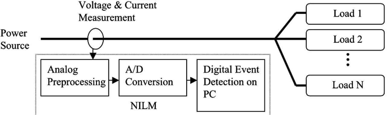
The NILM makes measurements of voltage and current solely at the utility service entry of a building, as shown in Figure 1. It characterizes individual loads by their unique signatures of power drawn from the mains. A transient detection algorithm can identify when each load turns on and off, even when several do so nearly simultaneously.
Load 1 Load 2 Load N Power Source Analog Preprocessing A/D Conversion Digital Event Detection on PC
Voltage & Current Measurement NILM Load 1 Load 2 Load N Power Source Analog Preprocessing A/D Conversion Digital Event Detection on PC
Voltage & Current Measurement
NILM
Figure 1: Block Diagram of Non-Intrusive Load Monitor
The transient behavior of a typical electrical load is strongly influenced by the physical task that the load performs. For example, Figure 2 shows the real power, 5th, and 7th harmonic
content demanded by a variable-speed ventilation fan drive in an HVAC machine room. It operates with a power electronic interface under active control, and represents systems deployed for energy conservation and active control in building machine rooms. Increasingly, variable speed drives (VSD) are appearing in residential air conditioning units. The drive begins with an “open loop” spin-up to operating speed during the first 40 seconds of operation. From 100 seconds on, the drive is operating under closed-loop control as it attempts to regulate the pressure in a distant duct by varying fan speed. Distinctive transient profiles like those shown below tend to appear even in loads that employ steady-state active wave-shaping, power electronic front-ends, active control, or power-factor correction. These transient shapes are indicative of the state and operating parameters of the electromechanical and electronic subsystems in the drive, and can be used as diagnostic indicators. For example, Figure 2 illustrates the steady-state oscillations in
nominal operation (after 100 seconds) that result from a poorly-tuned control loop. These
oscillations are relatively slow and easily missed by a casual inspection of the VSD control panel, but are easily detected by the NILM with transient event detection.
Figure 2: Turn-on transient of a power electronic variable speed drive.
Figure 3 shows a screen print from a prototype, real-time, load monitor. Four loads, including two induction motors and two different types of fluorescent lamp banks, are activated at nearly the same time. As shown in Figure 3, once trained with fingerprint signatures for the loads to be identified, the prototype event detector is able to recognize the turn-on transients of all four loads strictly by examining the aggregate traces of real power, reactive power, and harmonic content at the service entry.
Nonintrusive electrical load monitoring for homes and commercial and industrial
buildings offers a comprehensive solution for a number of problems. Monitoring from a single or limited number of measurement points reduces metering and installation cost. The NILM’s transient event detector permits identification of the operating schedule of individual loads from aggregate data, enabling detailed energy-scorekeeping. As a centralized computation and
monitoring portal, the NILM is an obvious platform for “smart” control of grid loads. The NILM extracts detailed information about the operation of individual loads, and could easily serve as a coordinator for managing demand-side consumption. The NILM is an information applicance, and can provide information over the web or a wireless network, enabling many different
“business models” for the use of disaggregated load consumption information. Home or facilities managers could use the information directly. With appropriate permissions, utilities can collect the information and offer more detailed billing or consumption analysis. Similar services could be offered by third party providers. Prognostic information can be developed from the NILM data for tracking load health and availability.
The possibility of creating three critical, missing pieces of hardware and software technology will be researched during this project to ready the NILM for use in the commercial marketplace: a new non-contact field sensor for easy installation in new and retrofit power monitoring; new signal hardware to make the NILM support all contemporary networking and information exchange systems; and software algorithms for using NILM data for fault detection and diagnostics of critical systems, particularly those with motors like HVAC plants.
Non-contact Sensor
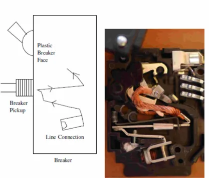
Closed or “clamp” core sensors wrapped around the utility feed typically provide the current sense signal for a NILM. These sensors prohibit widespread monitoring because skilled labor must separate Line and Neutral in order to deploy a wrap-around magnetic field sensor, even in the case of separable core sensors. We propose an alternative to traditional clamp or Hall-effect sensors. This alternative requires no skilled installation. This new sensor measures the current in the utility feed by sensing the resulting magnetic field at the face of the main (or other) circuit breaker in a standard breaker panel, where the Line and Neutral are already separated. The sensor can be interrogated through the steel panel door with no direct electrical contact, as the door must be closed to comply with safety regulations. Our connection to the front face of a circuit breaker is shown schematically on the left in Figure 4. The photograph on the right in Figure 4 shows the internal mechanism of a typical circuit breaker. The convoluted path of current through the protection gear inside the breaker makes a magnetic field that can be detected without electrical contact outside of the plastic breaker face. While breakers differ
slightly in construction, our survey of dozens of commercial breakers indicates that this approach will work with little or no modification in most circuit breaker panels in at least North America.
Figure 4: Circuit breaker pickup and typical circuit breaker (opened for illustration). The circuit breaker and circuit breaker pickup coil are shown schematically at the far right in Figure 5. The circuit breaker pickup is small and fits between the panel door and the front face of the breaker. The complete sensor shown in Figure 5 consists of three main parts: an inductive pickup for sensing current from the breaker face (Breaker Pickup), an inductive link designed to transmit power through the steel breaker panel door (Through-door Inductive Link), and a balanced JFET modulator circuit for transmitting information through that inductive link (JFET Mixer).
The outer coil is driven with a high-frequency sinusoidal carrier voltage. That voltage couples to the inner coil through the inductive link and drives a new JFET mixer. The JFET mixer controls the amount of current drawn from the inner coil, modulated by the low-frequency (60 Hz) current signal measured by the breaker pickup. The result is a modulation between the high frequency carrier signal and the low-frequency (60 Hz) signal measured at the breaker face. The external sense circuit monitors the current drawn through the inductive link to extract the resulting modulated signal. The internal device is fully powered by the applied carrier, and the entire system works without modification to the breaker panel or the circuit breaker itself. With
the modulated signal available to the sense circuit external to the door, the current through the main breaker can be analyzed by the NILM for load identification and power monitoring.
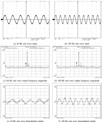
Our preliminary experiments use test equipment (spectrum analyzer, signal generator, etc.) to demonstrate this concept. Preliminary results are shown in Figure 6.
Figure 6: Preliminary experimental results: Currents through the breaker are shown in the top two plots (for 60Hz and 100Hz current signals, the 100 Hz representing distortion content). The middle plots show the spectrum of carrier and modulation, and the bottom plots show the reconstructed current signal outside of the breaker panel.
One goal of this project will be to construct a full, inexpensive, custom circuit
(eliminating test equipment in the demonstration) and breaker pickup system that can measure, reconstruct, and transmit observed breaker currents with a minimum 1 kHz bandwidth and a minimum 50dB dynamic range. This current sensor will simply attach magnetically to the door or panel wall of a circuit breaker panel, read the currents from a breaker, and provide this information outside of the panel enclosure to a monitoring system. It will enable a monitor to be installed in seconds by unskilled labor. A voltage measurement will be derived from a nearby plug outlet, where the “outside the panel” electronics will be powered. This new sensor will permit immediate access to current measurements safely at low cost and will enable many monitoring and control scenarios, including quick installation of a NILM.
Spectral Envelope Preprocessing Hardware
Direct examination of current waveforms may not be the best choice for many stages of some monitoring and control applications, including many components in energy scorekeeping, monitoring, or conservation systems. Direct operations on the current waveform require sample rates adequate to capture the highest harmonic content of interest [12]. In some metering, monitoring, and control applications it is more practical either to store data for a period of time and examine it later, or to transmit data to another location for interpretation and control. In either of these cases, it is convenient to have a useful representation of the data that avoids excessive storage or communication bandwidth requirements.
Spectral envelopes represent the time-varying harmonic content of waveforms, e.g., observed current waveforms. Spectral envelopes are illustrated in Figures 2 and 3 for the currents consumed by the associated loads. They provide a useful separation between data collection and analysis. They will permit a small, inexpensive system with low processing power to collect data continuously. A system with larger available processing power, potentially physically remote from the data collection front-end, can either review a storage device at a later time or continuously process a relatively low bandwidth information stream over a convenient communication channel, wired or wireless.
The spectral envelopes of current represent the harmonic content of the input waveform for each line-locked period of the service voltage. Given N samples i[n] of a waveform i(t) over one period, the samples can be expressed in terms of their spectral content by
Where the spectral envelopes ak and bk for that period are defined by
Here, k denotes the multiple of the line frequency to which a particular spectral envelope corresponds; for example, k = 1 corresponds to the 60 Hz component and k = 3 to the
180 Hz component. The values of these spectral envelopes are calculated for each period of the line voltage; the values at period m will be denoted ak[m] and bk[m]. With this definition, spectral
envelopes can naturally be calculated from the real and imaginary parts of the Discrete Fourier Transform (DFT) [17] of i[n] over each period of the line voltage.
In situations where the significant or relevant current drawn by an electrical load consists predominantly of the fundamental frequency (the frequency of the service voltage, for example, 60 Hz) and a small collection of the line frequency harmonics (such as the 2nd, 3rd, 5th), it is reasonable to record, for each period of the service voltage, only a few DFT coefficients. This approach has proven to provide excellent results for power tracking and for monitoring power quality and current distortion in our field tests. These relatively few DFT coefficients can be used to reconstruct the original current samples with a relatively small error. Furthermore, rather than reconstructing the original current waveforms, the time-varying values of the DFT coefficients themselves can be used directly as fingerprint signatures for the loads, or to track important quantities associated with load operation, with reasonable accuracy.
Because only a few DFT coefficients may be needed to accurately represent the current waveforms, this “spectral” approach to the representation of the waveforms serves as a form of compression. As a concrete example, consider current and voltage samples that are collected at a 7.68 KHz sample rate. The sampling rate provides adequate anti-aliasing without filtering effects and provides adequate detection of voltage zero crossings to enable line-locked data collection. This corresponds to 128 samples per 60 Hz line-cycle (N = 128), and so 64 meaningful complex DFT coefficients need to be stored to perfectly reconstruct arbitrary current samples. However, for many applications, including load monitoring for diagnostics, only a limited number of DFT coefficients need be stored. In field studies we have found that 4 coefficients, or 6.25% of the full set of already compact harmonically related DFT coefficients, were sufficient for most appliations.
Spectral envelopes can be directly interpreted as other meaningful physical quantities. If the voltage is not stiff or harmonically pure, it is possible to accurately estimate real and reactive power by storing a corresponding set of DFT coefficients of the voltage. That is, if the 1st, 3rd, 5th,
and 7th DFT coefficients of current are stored, then these same DFT coefficients of voltage should also be stored). For a discrete-time system, real power is given by
where i[n] and v[n] are the samples of current and voltage, respectively, over one period of length N. Reactive power can be calculated in an analogous fashion. Other combinations can be use to estimate harmonic distortion, crest factors, and other quantities of interest.
To calculate, store, and communicate a relevant subset of DFT coefficients for power monitoring and energy scorekeeping, we intend to design and construct a custom integrated circuit suite for energy monitoring using an FPGA as a computation core during the project period. We will develop an algorithm for computing spectral envelopes accurately in integer arithmetic easily implemented on an inexpensive FPGA, e.g., a low-cost Altera Cyclone I, EP1C3T100C8. The full spectral envelope preprocessor will consist of an analog-to-digital converter, and FPGA controller, and a WiFi/Ethernet/Wireless interface that can communicate through many different standards with ease, i.e., 802.11, Zigbee, or Bluetooth connections. Data can also be stored for later retrieval on a storage media such as a compact flash (CF) card.
The spectral preprocessor will consist of four subsystems show in the overall block diagram in Figure 7.
Figure 7: Spectral envelope preprocessor overview.
The transducer interface circuitry shown in Figure 7 could be, but is not limited to, the “contactless” circuit breaker pickup described previously. With the addition of the spectral envelope preprocessor, the circuit breaker pickup becomes quickly installed wired or wireless power monitor with low transmission bandwidth requirements.
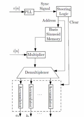
Figure 8: Preprocessor core block diagram.
Figure 8 shows a block diagram of the proposed FPGA-based spectral envelope preprocessor core. The preprocessor takes the discrete time samples of i(t) and v(t) as input, denoted i[n] and v[n] respectively, where n indexes the samples, and produces estimates of the spectral envelope coefficients ak and bk of the current i[n]. The voltage samples v[n] are used as input to a phase-locked loop (PLL), which synchronizes the entire computation to the line voltage. The output of the PLL is sent to a block of steering logic on the FPGA that produces the address for the basis sinusoid memory, as well as a clear signal for the accumulators. The basis sinusoid memory consists of the samples of the various basis sinusoids. The address produced by the steering logic specifies a single sample time of a single basis sinusoid. The sample of the basis sinusoid that is retrieved from the basis sinusoid memory is then multiplied by the current sample i[n]. The result of this multiplication is then passed through a demultiplexer which sends the result to the appropriate accumulator by using the address produced by steering logic to determine which spectral envelope coefficient is currently being calculated.
Our second project goal is to design and construct the FPGA-based system discussed above to calculate, store, and transmit spectral envelope data. To make use of this data, a monitoring or control system will typically include a subsystem to receive and use the spectral envelope data. For example, a homeowner could use a personal computer to collect spectral
envelope data from the FPGA preprocessor installed near or in a circuit breaker panel. The utility could collect spectral envelope information that is either stored and recovered periodically or transmitted wired or wirelessly as convenient. Our prototype will include a PC-based software application that can interface with the FPGA-based preprocessor via wired or wireless
communication channels, retrieve spectral envelopes, and display spectral envelope data.
Fault detection and diagnostics
Our third goal is to apply the hardware, signal processing algorithms, and software implemented in the first two tasks to develop fault detection and diagnostic algorithms for important energy consumers. This task will have two important impacts. First, it will enable prognostic and diagnostic identification of impending or occurring faults for some systems, and, second, it will ensure that these faults do not result in energy waste. Space limitations prevent a full description of all systems of interest to be studied during the project. We focus on our planned demonstration on HVAC systems in this section.
HVAC systems are outstanding targets for FDD. They are “mission critical” in many buildings in the sense that some buildings may not be able to be occupied without operating HVAC. HVAC systems can also be astonishing wasters of energy. They typify a class of systems that operate under feedback control. Even when a plant is damaged or operating outside of nominal specifications, the feedback control will run the plant to maintain a comfort setpoint, regardless of the energy needed to achieve this setpoint with a damaged but not completely broken machine plant. Over time, the energy wasted can be extraordinary.
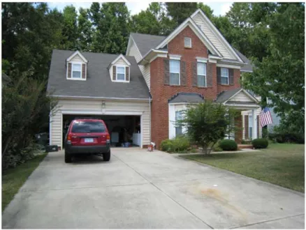
To illustrate our approach for nonintrusive diagnostic methods to be developed during this research, a set of exploratory experiments were performed on a residence located in North Carolina. This location was chosen for the climate conditions in the venue, which encourage residential occupants to make extensive and costly use of HVAC. A photograph of this house is shown in Figure 9. The house has approximately 2000 square feet of internal floor space, and is cooled by a central air-conditioning system which is divided into two zones: one air handler serves the ground floor, while the other air handler serves the second story. Both of these air handlers are installed in the attic, and flexible ductwork was used to distribute the cooled air from these air handlers throughout their respective zones.
Figure 9: Test home for preliminary FDD experiments with HVAC.
A Copeland single-phase capacitor-run scroll compressor (model no. CR22KF-PFV-130) was used in each refrigerant loop, with R-22 used as the refrigerant. The information on the nameplate of the condensing unit stated that the units were shipped with 62 oz of refrigerant; this represents the proper refrigerant charge for 30 feet of liquid line. After determining that 42 feet of tubing were required to span the distance between the compressor and the air handler in the attic, an additional 6.96 oz of refrigerant were added to the nominal system charge, so that the total system charge was 68.96 oz of refrigerant.
The compressor power was monitored on the power system where a NILM might be installed. Additional thermal instrumentation was also installed in order to monitor the local variations in temperature, humidity, and sunlight, which could affect the cooling load on the air-conditioning system. Our goal in the proposed work is to develop observers that eliminate the need for these additional sensors, deriving all needed information from nonintrusive electrical measurements. In the course of the data analysis, it became clear that a number of useful diagnostic methods could be formulated solely by using, at most, measurements of compressor power and the outdoor and indoor air temperature. We hope to eliminate the temperature measurements by using the compressor’s electrical behavior as its own temperature sensor. The small number of sensors which were needed for these preliminary diagnostic experiments was encouraging, as small numbers imply the possibility of creating an inexpensive FDD system for energy conservation.
Preliminary results to see if it was possible to identify undercharge faults in the
compressor operating time versus outdoor-indoor temperature difference behavior in both fully charged and undercharged states are shown in Figure 10 a and b. As these analyses are all based upon observations made from the fused datasets, it is helpful to illustrate the sets of temperature and electrical power data for two representative days in order to point out some of the particularly relevant features. To this end, the behavior of the fully charged system over one day is shown in Figure A, and the behavior of the undercharged system over one day is shown in Figure B. Three sets of data are illustrated in these figures: the outdoor temperature, the indoor temperature, and the electrical power input to the compressor. The compressor's cycling behavior can be
calculated from this plot by analyzing the times that it turns on and off. The average steady-state power consumption of the compressor over each cycle of operation is also illustrated in this plot.
Figure 10: Test results with correctly charged (left, “a”) and undercharged systems (right, “b”). One of the first notable observations that arises from an examination of these two days is that “delta T” has both positive and negative values. During the early hours of the morning, the indoor temperature is higher than the outdoor temperature, while the outdoor temperature is higher than the indoor temperature during the middle of the afternoon. Furthermore, it is interesting to note in both of these figures that the indoor temperature does not oscillate between two fixed values, but that these thresholds appear to gradually increase as the outdoor temperature increases. This is most likely an effect caused by the slow thermal behavior of the indoor
temperature sensor, rather than a behavior of the system itself. The changes in the steady-state compressor power with temperature are also quite noticeable; this effect is largely due to the fact the compressor load increases due to the higher pressures in the condenser caused by the higher
outdoor temperatures. This increase in the load on the compressor causes the compressor's power to increase commensurately.
One additional pertinent observation that can be made by examining the cycling behavior of the compressor in Figure A between approximately 1:00 pm and 10:00 pm is that the
compressor appears to be running for an hour continuously, and only shutting off for extremely brief periods of time. This apparent behavior is actually a processing artifact that was
intentionally introduced into the data to improve the performance of the FDD method. Because the compressor ran continuously during this time interval, it was necessary to develop a method of processing the data that could incorporate the local changes in the temperature. Compressor run-times that extended for longer than an hour were therefore broken into hour-long pieces, so that the compressor apparently turned off and on within the same second in the processed data. This made it possible to calculate the average temperature over the interval of an hour, which was much more representative of the system's behavior.
In comparing the data representing the fully charged system and the undercharged system, significant differences between the cycling behavior on each day are apparent even in the unprocessed data. For example, though undercharged test day is approximately 2 degrees Celsius cooler than correctly charged day, the compressor runs for a longer interval of time in the middle of the day (from 12:00 pm to 11:00 pm), than the fully charged system does (which runs from 1:00 pm to 10:00 pm). While these days are intended only to illustrate the representative behavior of the system, this strongly suggests that refrigerant undercharge detection methods that use nonintrusive observations of the cycling behavior will be able to successfully distinguish the behavior of a fully charged system from the behavior of an undercharged system.
During the proposed project, we intend to use the monitoring hardware to collect data for new FDD algorithms that we will develop during the performance period. These FDD algorithms will be demonstrated on HVAC systems, and other important building loads including lighting, pumps, and office equipment.
1.2 Current State of Knowledge or Technology Regarding NILM:
One of the earliest approaches to non-intrusive monitoring, developed in the 1980's at MIT by Professor Fred Schweppe and Dr. George Hart, had its origins in load monitoring for residential buildings. The operating schedules of individual loads were determined by Dr. Hart’s
ingenious scheme of identifying times at which a near-constant series of electrical power measurements changed to another near constant series. Changes were characterized by their magnitude and sign in real and reactive power. Changes of near-equal magnitude and opposite sign were paired to establish the operating cycles and energy consumption of individual appliances. The detection of changes in quasi-steady-state demand provides the basis for a commercial version of this early work, described in a 1999 article in the IEEE Computer Applications in Power [26].
This 1999 CAP article describes a five-step process for load disaggregation through the detection of changes in aggregate power consumption. First, an edge detector is used to identify changes in quasi-steady-state levels. These changes presumably correspond to the turn-on or turn-off of individual or groups of loads. Second, a cluster analysis is used to locate these changes or events in a two-dimensional “signature space” of real and reactive power (a P- Q plane). Third, positive and negative clusters of similar magnitude are paired or matched
(especially for “two-state” loads that simply turn-on, consume a relatively fixed power, and then turn-off). Anomaly resolution is accomplished as a fourth step in which unmatched clusters and events are paired or associated with existing or new clusters according to a best likelihood algorithm. Finally, in the fifth step, pairs of clusters are associated with known load power consumption levels to determine the operating schedule of individual loads. This association is determined using information gathered during a training or survey phase in the building. The signature space reduces the potentially complex, rich data in load transients to a two-dimensional space of changes in power consumption. This technique has a pleasing graphical interpretation, and has been shown to work well in certain types of buildings, especially residences. Recent field tests have underscored some well known, and other not so well known, limitations of the
technique of examining steady-state changes in a signature space.
The two-dimensional steady-state signature technique relies on at least three key assumptions that ultimately limit the method. The first assumption is that different loads of interest will exhibit unique signatures in the P-Q plane. They may not. This is especially true in commercial and industrial facilities, where load balancing, power factor correction, and a multiplicity and variety of loads far in excess of the mix found in typical residences all conspire to limit the distinction of different load signatures. In a home, there may be only one 5000-watt load, an electric water heater, for example. A commercial facility with a full HVAC plant, office equipment, and lighting banks may have several different loads with overlapping clusters in the P-Q plane.
The second assumption is that it is possible to define a notion of quasi-steady-state consumption and to detect changes in consumption level. In challenging commercial and industrial environments where loads may be turned on and off frequently, it has proven difficult in the field to reliably bound either a maximum or a minimum time interval to wait before declaring the power consumption to be “steady.” A conservative choice might demand a relatively long time of near-constant-power demand before declaring a steady-state power level. Longer waiting times mean that the monitor will not be able to individually track changes during high rates of event generation, and many events may be missed. These events may or may not be caught during anomaly resolution. Relatively short waiting times, on the other hand, may trigger the recording of a change in steady state consumption in the building before a load transient is complete, leading to the inclusion of spurious events in the cluster analysis. We have found loads like fans and chillers in large HVAC plants that might take 30 seconds or several minutes to spin-up gradually to operating speed. Other loads, like variable speed drives, may never settle to a steady-state level at all, and, if large enough in variation in power consumption, could prevent the monitor from ever declaring a steady-state consumption level or recording any events. Still other loads, which should settle to a steady-state level, may not if they include poorly tuned controllers or other diagnostic problems.
Also, although not a requirement of the five-step disaggregation procedure, most implementations to date operate in a “batch” mode on a day or more of stored event data before performing clustering, matching, and identification. This approach makes the third assumption that near-real-time identification of load operation is not necessary. This essentially limits the monitor to use in load survey and scorekeeping applications, excluding applications in real-time diagnostics.
A typical residence contains a relatively small number of distinctive loads. The rate of event generation is determined by a small number of occupants and tends to be low. The three assumptions have therefore proven reasonable in the field. Typically, homes and small businesses can be surveyed non-intrusively with great success. Enetics Incorporated has
commercialized this technology and sells it under the trademark SPEEDTM (Single Point End-use
Energy Disaggregation).
No commercially available system offers the ease of installation, flexibility, real-time access, and richness of information for energy scorekeeping and diagnostics that the proposed system will deliver. No commercial or research system offers the combination of hardware and
software for power monitoring, or the ease of both new and retrofit monitoring, that the proposed system will offer.
Regarding HVAC FDD:
The first researchers to systematically investigate the faults that are responsible for
malfunctioning vapor compression air conditioning equipment were Cunniffe, James, and Dunn [25]. The authors of this paper conducted a survey of vapor compression refrigeration plants in a variety of different applications, such as low temperature refrigeration applications, air
conditioning systems, and vehicle refrigeration systems, in order to quantify and enumerate the common faults which occur. Rather than quantify the statistics of particular faults, the ultimate causes of the faults were classied; of the 851 systems which were studied, 32% of the mechanical faults and 29% of the electrical faults were caused by unforeseen operating conditions. In
comparison, 38% of the mechanical faults and 44% of the electrical faults were caused by faulty materials, manufacture, design, installation, service, commissioning, or maintenance. The remainder of the faults were either due to normal deterioration or remained unclassifed. As these statistics were collected, the authors observed that a number of operational faults overloaded the compressor, which consequently failed and was diagnosed as the faulty component.
This type of failure is problematic because the compressor is often repaired without fixing the underlying fault. In order to address this concern, the authors identify a number of fault classes which cause overloading. High discharge temperatures represent one class of faults which account for 9-15% of the failures in reciprocating compressors, which are in turn caused by faults such as high intermittent plant operation, fouled condenser surfaces, non-condensible gases, or other unforeseen operating conditions. Liquid return to the compressor housing and refrigerant migration, in which liquid refrigerant accumulates in the compressor shell and then boils up into the compressor cylinders, can also cause a host of problems, ranging from increased discharge temperatures, to major mechanical damage, to the degradation of winding insulation. Poorly controlled expansion valve or evaporator dynamics, excessive equipment cycling, and inadequate system cleanliness also caused compressors to fail prematurely.
The next researchers to systematically investigate the faults in air conditioning equipment were Stouppe and Lau [29]. They examined 15,760 failures in units with a cooling capacity up to 50 tons (600,000 BTU/hr) over the course of eight years (1980-1987) by scrutinizing insurance claims which were filed for the repair of air conditioning equipment. Many different types of
refrigeration systems were examined, incorporating both reciprocating and centrifugal
compressors. Of the 15,760 failures examined, 12,518 had their specific cause of failure denoted on the claim. The authors found that these units generally failed when they were approximately 10 years old, and that such units had no major inspections or overhauls over that entire period of time. Furthermore, 11,349 of the failures were electrical (comprising motors, controls, and electrical apparatus), while 4,411 were mechanical (compressor bodies, system piping, or vessels). The authors specifically examined the causes of failure for hermetically sealed air conditioning and refrigeration units: 76.6% of the failures were electrical (motor windings, control equipment, and other associated issues), 18.9% were mechanical (compressor valves, springs, bearings, connecting rods, pistons, crankshafts, lubrication), and 4.5% of the failures were caused by malfunctions in the refrigerant circuit. A few particular notes were also made trends which were observed in the causes of compressor motor failure. Insulation deterioration on the motor windings due to age and/or service, as well as unbalanced voltage and single phase operation were some of the main causes of the failure; degradation in motor stator windings was by far the most prevalent cause of motor failure, accounting for 84% of failures in hermetic motors and 74% in the non-hermetic motors. The remaining causes of the failures were generally broken rotor bars, bearings, and motor control equipment. Of the motor control failures, 168 failures were directly attributed to short cycling, or the repeated starting and stopping of the motor many times in rapid succession.
A more detailed study of mechanical compressor failures for reciprocating freon-based units showed that the bulk of the failures could be attributed to two main causes. The first of these causes is that of metal fatigue in the internal suction and discharge valves and springs, due to the hundreds of millions of operating cycles that these parts see over the average lifetime. Liquid slugging, or the unintentional injection of liquid refrigerant into the cylinder, was also the direct cause of 20% of the mechanical failures, due to the hydraulic forces from the attempt to compress the incompressible liquid refrigerant which acts on the valves, valve plates, pistons, and
connecting rods. Under normal operating conditions, gaseous refrigerant is pulled into the cylinder during the intake cycle, but when liquid refrigerant enters, these hydraulic forces can cause broken valves and valve plates, as well as cascading damage to all of the mechanical parts of the compressor.
Braun and Breuker [29] examined two different types of faults in package rooftop air conditioners: those which caused the air conditioner to run inefficiently, but did not cause the equipment to cease operation, and those in which the RTU could no longer operate mechanically or electrically. By analyzing a statistically representative subset of a database containing 6000
separate faults observed from 1989 to 1995, the authors found that, of the fault classifications which resulted in “no air conditioning,” or faults in which the unit was running inefficiently but was still electrically and mechanically operational, 60% were caused by electrical problems (such as motors and control problems).
These three different failure analyses, examining a total of over 20,000 failures in rooftop air conditioning units, provide some keen insights into the requirements of a fault detection and diagnostic system. It is clear that a method of identifying di_erent modes of failure in compressor assemblies and motors would have a significant impact upon overall RTU performance and service time, as the system could alert a service technician to the cause of failure, rather than relying upon the technician's troubleshooting expertise. As many faults, such as liquid slugging, degrade the compressor performance over an extended period of time, an FDD system may also be able to greatly reduce the average repair cost by alerting the user to early instances of the fault condition. This can potentially save a great deal of money, since the lifetime of the compressor could be substantially lengthened. In addition, not all of the faults would have to be _xed by an HVAC technician, as an FDD system which could properly identify blocked evaporator and condenser coils and alert a building mechanic could also save a considerable amount of money for unnecessary service calls.
The NILM platform could dramatically extend the capabilities of such an FDD platform for package air conditioning units, due to its ability to detect purely electrical faults, as well as its ability to detect changes in electrical transients due to variations in the mechanical or thermal load which are coupled to the electrical power.
2. ENERGY, ENVIRONMENTAL AND ECONOMIC BENEFITS 2.1 Energy Savings
As mentioned above, there are two major sources of energy savings in buildings: good housekeeping on the part of end-users and improved operation of space-conditioning equipment. The former category relies on turning off equipment that is not needed, including HVAC fans in offices, lights, and office equipment, for example. The latter includes proper scheduling of central HVAC equipment, making use of outdoor air for free cooling when weather permits, and prompt detection and correction of faults that affect energy performance, including fouled cooling coils, stuck or leaky dampers and valves, and chiller vacuum or refrigerant leaks.
A relatively recent example of the benefits of housekeeping, as applied to occupant and HVAC loads, comes from California, where building power demand shrunk by about 9% in 2001.
(The California Energy Commission reported a 9% reduction in demand in 2001 relative to 2000, adjusted for weather and growth.) This demand reduction was the accumulated effect of many individual, low-technology actions. On the HVAC side, researchers in Texas have shown that, with very little capital investment, better commissioning of HVAC equipment and ongoing detection of major problems can reduce energy consumption by at least 20% [24].
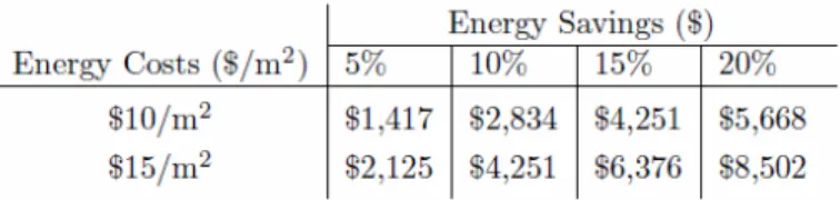
The studied building has 2,834 square meters of floor area. Based upon a two-week building study, the yearly energy consumption of the building is approximately 633 MWh. Assuming a typical electric rate of $50/MWh, this translates to roughly $31,000/year, or $11 per square meter. This estimate is conservative, however, as the energy consumption was calculated by using only real power, while the utility often also charges commercial buildings for the amount of reactive power consumed. Other factors which are not included are the variability in the electric rate, as well as the fact that this average was computed for two weeks at the beginning of April, which does not include the higher electricity usage from the summer cooling load. This estimate for the yearly energy consumption of the building is therefore very conservative. The NILM's potential to improve building performance in the face of the uncertainty of these estimates may be evaluated by using estimates which have been calculated by surveying the energy consumption of a wide array of commercial buildings. Such surveys report that the annual energy costs in buildings are typically $10-$15 per square meter (The Energy Information Agency of the U.S. Department of Energy reported electricity expenditures of $10.85 per square meter in 1999 for commercial buildings and $13.04 per square meter for all fuels). In order to examine the potential savings that could be realized by installing a NILM to monitor energy consumption, a wide range of results is tabulated below for yearly energy uses of $10, $15, and $20 per square meter.
Table 1: The cost savings potentially realized by a NILM due to an energy savings as a percentage of the yearly energy consumption.
The estimated savings in Table 1 can be compared to those measured by others. Texas A&M University researchers reported a savings of $2.37/m2 due to improved operations in seven Texas office buildings [23]. Savings at this level would yield about $6,700/year in the studied building, corresponding to the entry in Table 1 for 15% savings at $15/m2. A NILM, as installed in a
representative building for the purposes of identifying and monitoring the building
commissioning process, would cost less than $1000 installed, without a subsequent energy-monitoring service. Such an installation could quickly pay for itself, as 15% reduction in energy consumption on a building which consumes $15 per square meter would result in an immediate net monetary savings between $2,000 and $3,000, and a considerably higher lifetime savings. The building owner could either make use of the meter itself, paying for software upgrades and maintenance as necessary, or subscribe to a service that would highlight opportunities for
conservation, track progress, and produce timely reports. Such a service might cost about 20% of the annual savings, or $800 per year.
A key element of such an approach is the active involvement of building occupants and energy services staff (those who maintain the HVAC equipment and those tasked with improved energy performance for an entire site). Someone needs to have incentive to do better, through financial reward (cost savings credited to operations accounts or otherwise used for the benefit of those who achieve the savings) or commendation. The NILM is a very useful and direct source of energy information, making it possible to track on a day-to-day basis the benefits of collective efforts to conserve energy.
BIBLIOGRAPHY & REFERENCES CITED
1. R.E. Abbot and S.C. Hadden, EPRI Final Report CU-6623, December 1989, “Requirements for an Advanced Utility Load Monitoring System.”
2. “The Smart Grid: An Introduction,” U. S. Department of Energy, http://www.oe.energy. gov/1165. htm, August 2009.
3. U.S. Patent Number 5,483,153, S.B. Leeb, et.al., Transient Event Detector for use in Nonintrusive Load Monitoring Systems.
4. Multiprocessing Transient Event Detector for Use in a Nonintrusive Electrical Load Monitoring System, S.B. Leeb, et.al., U.S. Patent Number 5,717,325. 5. Shaw, S.R., S.B. Leeb, L.K. Norford, R.W. Cox, “Nonintrusive Load
Monitoring and Diagnostics in Power Systems,” IEEE Transactions on Instrumentation and Measurement, Volume 57, No. 7, July 2008, pp. 1445-1454.
6. S. B. Leeb, S. R. Shaw, and J. L. Kirtley, “Transient event detection in spectral envelope estimates for nonintrusive load monitoring,” IEEE Trans. Power Del. vol. 7, no. 3, pp. 1200-1210, Jul. 1995.
7. Khan, U. A. , S. B. Leeb, M. C. Lee, “A Multiprocessor for Transient Event Detection,” IEEE Transactions on Power Delivery, Volume 12, Number 1, pp. 51-60, January 1997.
8. S. R. Shaw, C. B. Abler, R. F. Lepard, D. Luo, S. B. Leeb, and L. K. Norford, “Instrumentation for high performance nonintrusive electrical load monitoring,” Trans. ASME J. Sol. Energy Eng. , vol. 120, no. 3, pp. 224-229, Aug. 1998.
9. S. R. Shaw, “System identification techniques and modeling for nonintrusive load diagnostics,” Ph. D. dissertation, Massachusetts Institute of Technology, Cambridge, MA, Feb. 2000.
10. Laughman, C. R., “Fault Detection Methods for Vapor-Compression Air Conditioners Using Electrical Measurements,” MIT BT Ph. D. thesis, September 2008.
11. Laughman, C.R., Leeb, S.B., Norford, L.K., Shaw, S.R., Armstrong, P.R., “A Two-Step Method for Estimating the Parameters of Induction Machine Models,” IEEE Energy Conversion Conference and Exposition, San Jose, CA, September 2009.
12. J. Paris, et al. “Scalability of Non-Intrusive Load Monitoring for Shipboard Applications,” ASNE Day 2009, National Harbor, Maryland, April, 2009. 13. A. P. Dempster, N. M. Laird, D. B. Rubin, “Maximum Likelihood from
Incomplete Data via the EM Algorithm,” Journal of the Royal Statistical Society, Series B 39:1-38, 1977.
14. U.S. Patent 5,212,441, “Harmonic-Adjusted Power Factor Meter,” May 18, 1993.
15. U.S.Patent 5,229,713, “Method for Determining Electrical Energy Consumption,” July 20, 1993.
16. U.S. Patent 5,548,527, “Programmable Electrical Energy Meter Utilizing a Non-Volatile Memory,” August 20, 1996.
17. U.S. Patent 6,615,147, “Revenue Meter with Power Quality Features,” September 2, 2003.
18. U.S. Patent 7,525,423, “Automated Meter Reading Communication System and Method,” April 28, 2009.
20. F. Itakura, “Minimum Prediction Residual Principle Applied to Speech Recognition,” IEEE Transactions on Acoustics, Speech, and Signal Processing, Vol ASSP–23, February 1975, pp. 67–72.
21. M.S. Breuker and J.E. Braun. Common faults and their impacts for rooftop air conditioners. International Journal of HVAC+R Research, 4(3):303-318, June 1998.
22. M.S. Breuker and J.E. Braun. Evaluating the performance of a fault detection and diagnostic system for vapor compression equipment. International Journal of HVAC+R Research, 4(4):401-425, October 1998.
23. D.E. Claridge, M. Liu, W.D. Turner, Y. Zhu, M. Abbas, and J.S. Haberl. Energy and comfort benefits of continuous commissioning in buildings. In Proc. of the Int'l Conf. Improving Electricity Efficiency in Commercial Buildings, Amsterdam, The Netherlands, September 1998.
24. D.E. Claridge, W.D. Turner, M. Liu, S. Deng, G. Wei, C. Culp, H. Chen, and S.Y. Cho. Is commissioning once enough? In Solutions for Energy Security & Facility Management Challenges: Proc. of the 25th WEEC, pages 29-36, Atlanta, GA, October 2002.
25. M. Cunniffe, R.W. James, and A. Dunn. An analysis of fault occurrence in refrigeration plant and the e_ect on current practice. Australian Refrigeration, Air Conditioning, and Heating, 40(7):36-43, July 1986.
26. S. Drenker and A. Kader, “Nonintrusive monitoring of electrical loads,” IEEE Computers Applications in Power, Vol. 12, No. 4. pp. 47-51, 1999.
27. D.E. Stouppe and T.Y.S. Lau. Air conditioning and refrigeration equipment failures. National Engineer, 93:14-17, 1989.
28. T. M. Rossi and J.E. Braun. A statistical, rule-based fault detection and diagnostic method for vapor compression air conditioners. International Journal of HVAC+R Research, 3(1):19-37, January 1997.
29. M.S. Breuker and J.E. Braun. Evaluating the performance of a fault detection and diagnostic system for vapor compression equipment. International Journal of HVAC+R Research, 4(4):401{425, October 1998.