Conservation in signal processing systems

Conservation in Signal Processing Systems

by

Thomas A. Baran

B.S. Electrical Engineering, Tufts University (2004)

B.S. Biomedical Engineering, Tufts University (2004)

ARCHIVES

OF TECHNOLOGY

JUL 0 1 2012

LIBRARIES

S.M. EECS, Massachusetts Institute of Technology (2007)

Submitted to the Department of Electrical Engineering and Computer Science

in partial fulfillment of the requirements for the degree of

Doctor of Philosophy in Electrical Engineering and Computer Science

at the

MASSACHUSETTS INSTITUTE OF TECHNOLOGY

June 2012

@

Massachusetts Institute of Technology 2012. All rights reserved.

Author ...

Department of Electrical Engineering and Computer Science

May 23, 2012

Certified by...

Alan V. Oppenheim

Ford Professor of Engineering

Thesis Supervisor

-, n ' If

Accepted by ...

S..

... . .

lie

A. Kolodziej ski

Conservation in Signal Processing Systems

by

Thomas A. Baran

Submitted to the Department of Electrical Engineering and Computer Science on May 23, 2012, in partial fulfillment of the

requirements for the degree of

Doctor of Philosophy in Electrical Engineering and Computer Science

Abstract

Conservation principles have played a key role in the development and analysis of many existing engineering systems and algorithms. In electrical network theory for example, many of the useful theorems regarding the stability, robustness, and vari-ational properties of circuits can be derived in terms of Tellegen's theorem, which states that a wide range of quantities, including power, are conserved. Conservation principles also lay the groundwork for a number of results related to control theory, algorithms for optimization, and efficient filter implementations, suggesting poten-tial opportunity in developing a cohesive signal processing framework within which to view these principles. This thesis makes progress toward that goal, providing a unified treatment of a class of conservation principles that occur in signal processing systems. The main contributions in the thesis can be broadly categorized as pertain-ing to a mathematical formulation of a class of conservation principles, the synthesis and identification of these principles in signal processing systems, a variational inter-pretation of these principles, and the use of these principles in designing and gaining insight into various algorithms. In illustrating the use of the framework, examples related to linear and nonlinear signal-flow graph analysis, robust filter architectures, and algorithms for distributed control are provided.

Thesis Supervisor: Alan V. Oppenheim Title: Ford Professor of Engineering

Acknowledgments

There are many that have shaped the path that this thesis took during my time at MIT, sometimes in very significant ways, and I would like to recognize a small subset of these people here.

I would first like to thank my thesis supervisor Al Oppenheim, who provided significant intellectual and moral support throughout the process of researching and writing this document. Al has the remarkable ability to simultaneously act as a men-tor, a critic, an advocate, a copy edimen-tor, a colleague, and a friend, and I know of few other people who can, with a single well-chosen comment, identify an elusive weakness in an argument in a way that ultimately leads to the argument being significantly strengthened. Al, thank you for teaching me how to do research, how to teach, and how to complete this thesis. It has been a joy working with you, and I look forward to many more years of collaboration and friendship.

It has also been wonderful to have had a thesis committee with expertise so well-matched to the thesis. To Paul Penfield: thank you in particular for numerous discussions where your insight into electrical network theory provided me with a complementary and ultimately very useful perspective into my research. To John Wyatt: thank you for taking the time to dig into the details of various arguments, and in particular for introducing me to the vector subspace view of Tellegen's theorem. There are many ways that you have both significantly impacted the development of this thesis.

There were many faculty and researchers at MIT and elsewhere with whom I had helpful conversations that influenced the writing, and I would like to especially thank (in alphabetical order): Ron Crochiere, Jack Dennis, Berthold Horn, Sanjoy Mitter, Pablo Parrilo, Tom Quatieri, Ron Schafer, George Verghese, David Vogan, and Jan Willems in this regard. In particular, the conversations with Berthold Horn led to a fitting example for applying some of the principles in this thesis, and conversations with Sanjoy Mitter seemed always to uncover useful references.

during my time here: Ballard Blair, Ross Bland, Petros Boufounos, Sefa Demirtas, Sourav Dey, Dan Dudgeon, Xue Feng, Kathryn Fischer, Zahi Karam, Al Kharbouch, Jon Paul Kitchens, Tarek Lahlou, Joonsung Lee, Jeremy Leow, Shay Maymon, Martin McCormick, Joe McMichael, Milutin Pajovic, Charlie Rohrs, Melanie Rudoy, Maya Said, Joe Sikora, Eric Strattman, Guolong Su, Archana Venkatraman, Laura von Bosau, and Matt Willsey. Thank you for making this a wonderful place in which to live and do research. In particular to Eric, Kathryn and Laura: thank you for your support of the DSPG in keeping it running smoothly and for being significant cultural contributors to the group. With specific regard to this thesis, I would like to thank the following members (in no particular order): To Ballard and Jon Paul: for a number of enthusiastic discussions during the formative stages of the thesis that helped it to take shape. To Dennis and Shay: for the many whiteboard sessions that played a key role in developing critical mathematical details in this thesis. And also to Dennis: for encouraging me to listen on John Wyatt's class about functional analysis and signal processing, which ultimately impacted the direction of the thesis. To Sefa and Guolong: for helpful conversations about equivalent conditions for strong conservation. To Zahi: for being an exemplary office mate and providing much-needed distractions. To Charlie: for discussions about life, the thesis, and related concepts in control theory. To Martin: for providing feedback about the variational principles in the thesis through discussions that were very helpful and interesting, so much so that I had to avoid our office during the intense stages of thesis writing. To Melanie: for being a great office mate for many years, and for establishing a precedent of wonderful food at the DSPG brainstorming sessions, a practice that continues to this day. To Petros, Dan, Xue, Tarek, Joe McMichael, and Milutin: for enthusiastic comments during the DSPG brainstorming sessions that were often instrumental in shaping the thesis. Also to the other members of the sixth floor, and in particular to John Sun and Daniel Weller: thank you for helpful discussions and for contributing significantly to the congenial atmosphere on the floor.

Part of what has made the process of writing possible is having a great group of friends, and I would like to recognize in particular Matt Hirsch and Louise Flannery

for being terrific roommates, especially so during the intense writing stages. Also to Matt: thank you for the many technical discussions around the kitchen table and elsewhere that were instrumental in shaping the thesis. I would also like to recognize Ryan Magee for providing an environment at Atwood's Tavern that was welcoming of my experimentation with sound and signal processing, and also that served as a great weekend distraction.

To my family: Mary, Mom and Dad, thank you for being a supportive part of my life. And especially to my parents: it is impossible to list all of the ways that you have been an impact. Mom, thank you for inspiring me to be creative through all of the creative things that you have done, and for instilling in me a healthy degree of perfectionism that I believe has served me well while writing this thesis. Dad, thank you for always being eager to answer my unending questions about life, the universe and Ohm's law during long family road trips, for having a contagious enthusiasm for technical things that influenced me at a very young age, and for nurturing that enthusiasm by working with me on many electronics projects. I feel very fortunate to have parents that have been so supportive of my interests, and you have both shaped this thesis in a big way. One of the things that has become customary in the DSPG is to include six words that summarize the process of writing the thesis, and often whose full meaning is known only to a handful of people. My six words are: "Half-gallon of milk, home in refrigerator."

Contents

1 Introduction

2 System representations and manipulations

2.1 Behavioral representations . . . . 2.2 Input-output representations . . . . 2.2.1 Linear and nonlinear signal-flow graphs . . . . 2.2.2 Interconnective systems . . . . 2.3 Im age representations . . . . 2.4 Manipulations between representations . . . . 2.4.1 Behaviorally-equivalent, multiple-input, multiple-output systems 2.4.2 Behaviorally-equivalent interconnections of functions . . . . .

2.5 Partial taxonomy of 2-input, 2-output linear systems . . . .

3 Conservation framework

3.1 Organized variable spaces . . . . 3.1.1 The correspondence map . . . . 3.1.2 Partition decompositions . . . . 3.1.3 Conjugate decompositions . . . 3.1.4 OVS definition . . . . 3.2 Examples of organized variable spaces . 3.2.1 Electrical networks . . . . 3.2.2 Feedback systems . . . . 3.2.3 Wave-digital interconnections . 13 17 17 18 19 21 24 26 26 33 35 37 . . . . 3 8 . . . . 3 9 . . . . 4 2 . . . . 4 3 . . . . 4 5 . . . . 4 6 . . . . 4 7 . . . . 4 9 . . . . 5 4

3.2.4 Lattice filters . . . . 58

3.3 Transformations on Q(x) and conservative sets . . . . 60

3.3.1 Relationships between transformations of OVS elements . . . 61

3.3.2 Canonical conjugate bases . . . . 63

3.3.3 Dp-invariant transformations . . . . 66

3.3.4 Q(x)-invariant transformations . . . . 69

3.4 Conservation over vector spaces . . . . 75

3.4.1 Strong conservation . . . . 75

3.4.2 The manifold of conservative vector spaces . . . . 82

4 Conservative interconnecting systems 85 4.1 Image representations of conservative interconnections . . . . 86

4.2 Comments on the structure of 9Q . . . . 93

4.2.1 Isomorphisms with O(L, L), SO(L, L) and SO+(L, L) . . . . . 93

4.2.2 The families T[q; T q'r ;t) and Tj generate all strongly-conservative vector spaces . . . . 94

4.2.3 The families T T/'r0, T;t, and Tf generate all conservative vector spaces . . . . 97

4.3 Generating matched conservative interconnecting systems . . . . 99

4.3.1 A condition for conservation . . . . 103

4.3.2 A condition for strong conservation . . . . 106

4.4 Identifying maximal-D, conservation in matched interconnecting systems111 4.4.1 Partition transformations for identifying and strengthening con-servation . . . .. . . 114

4.4.2 A strategy for identifying transformations . . . . 117

4.4.3 A strategy for strengthening weak conservation . . . . 122

4.4.4 Identifying conservation in a bilateral vehicle speed control system 124 4.4.5 Obtaining all conservation laws for a conservative behavior . . 129

5 Variational principles of strongly-conservative spaces 133 5.1 OVS content and co-content . . . . 135

5.1.1 D efinition . . . .

5.1.2 Relationship to integral definitions . . . . 5.1.3 Composing f(y) and g(y) as functions on subvectors . 5.1.4 Re-parameterizing f(y)-g(y), f(y)-Q(y) and g(y)-R(y)

5.1.5 Some example contours . . . .

5.1.6 _{Functionally-related f(y)-Q(y) and g(y)-R(y) contours}

5.2 Connections with optimization theory . . . .

5.3 Dynamics of OVS content and co-content . . . .

6 Examples and conclusions

6.1 _{Inversion of feedback-based compensation systems . . . .} 6.2 A generalized Tellegen's theorem for signal-flow graphs . . . . 6.3 The set of lossless wave-digital building blocks . . . . 6.4 Linearly-constrained p-norm minimization . . . .

6.5 A distributed system for vehicle density control . . . .

A Proof of Thm. 3.1 B Glossary of terms . . . . 136 . . . . 143 . . . . 147 contours149 . . . . 151 . . . . 155 . . . . 162 . . . . 163 173 173 176 181 184 187 195 201

Chapter 1

Introduction

Conjugate effort and flow variables are deeply connected to our understanding of physical systems. Also referred to as "effort" and "flow" variables or "across" and "through" variables, conjugate variables represent physical quantities that when mul-tiplied together indicate the amount of power consumed or generated by a given system. In physical systems that are assembled as a lossless interconnection of physi-cal subsystems, the total power consumed or produced by the interconnection is zero, i.e. power is conserved. A lossless physical interconnection of K subsystems, each with conjugate effort and flow variables denoted ek and fk respectively, therefore has a conservation law that may be written as

elfl + - - -+ eKfK 0(1.1)

In such physical systems, Eq. 1.1 holds independent of whether the interconnected subsystems are linear or nonlinear, time-invariant or time-varying, or deterministic or stochastic. As such, the use of Eq. 1.1 in the derivation of useful mathematical theorems about physical systems often implies not only that the theorems apply very broadly, but also that the application of linear or nonlinear transformations may be used as a tool in the corresponding derivations. And furthermore, such transformations may be used to modify existing theorems in arriving at additional related results.

One may look to electrical networks to find a very broad class of such theorems originating from equations of the form of Eq. 1.1. In this class of physical systems, Eq. 1.1 is embodied by Tellegen's Theorem, [34] and a comprehensive summary of many of the accompanying theorems, which address among other things stability, sen-sitivity, and variational principles in electrical networks, is found in [31]. Eq. 1.1 also forms a cornerstone of the bond graph methodology, applied widely in the analysis, design and control of mechanical, thermal, hydraulic, electrical, and other physical systems. [30,35] The bond graph framework has also been applied in the analysis of social and economic systems as well. [6]

In contrast to physical systems, many current signal processing architectures, including general-purpose computers and digital signal processors, implement algo-rithms in a way that is often far-removed from the physics underlying their imple-mentation. One advantage to this is that a wide range of signal processing algorithms can be realized that might otherwise be difficult or impossible to implement directly in discrete physical devices, including for example transform-based coding, cepstral processing, and adaptive filtering. However, the high degree of generality facilitated by these types of architectures comes with the expense of losing some of the powerful analytic tools traditionally applied in the design and analysis of the restricted set of systems that is allowed physically, and derivations of many of these tools stem from equations of the form of Eq. 1.1.

A common strategy to overcome this essentially involves designing signal process-ing algorithms that mimic the equations or sets of equations describprocess-ing a specific physical system or class of physical systems. Any signal processing algorithm that can be put in the form of the equations is then regarded as being of a special class, to which a wide range of theorems often apply. For example, the class of signal process-ing systems consistprocess-ing of two subsystems interconnected to form a feedback loop is a canonical representation into which it is often desirable to place control systems, and about which many useful results are known. And in the early work by Zames [43,44] describing open-loop conditions for closed-loop stability in this class of systems, the equivalent electrical network is often referenced.

Another class of signal processing algorithms developed in this spirit is the wave-digital class of structures, which are based on the equations describing physical mi-crowave filters, and which have exceptional stability and robustness properties, even in the presence of parameter perturbations. [18] These properties were originally proven

by drawing analogies to reference physical microwave systems, which are known to

have similar characteristics. [17] The stability properties of other signal processing structures, such as lattice filters, have likewise been determined by manipulating them to fit the form of the equations describing wave-digital filters.

This strategy has also been used in the field of optimization. The network-based optimization algorithm developed by Dennis to solve the multi-commodity network flow problem was derived by designing a reference electrical network, with the network "content" being equivalent to the cost function in the original optimization. [14,15] Chua also discussed the use of nonreciprocal elements such as operational amplifiers in realizing the idealized components in Dennis' formulation, in addition to those required in a broader range of nonlinear problems. [8,9] In Dennis' work, the question of finding an optimal set of primal and dual decision variables, shown by Dennis to be equivalent to voltages and currents in the network, also involved ensuring that the network would indeed reach steady state, i.e. it involved ensuring stability of the network. Theorems regarding the stationarity of network content and the stability of electrical networks can be derived by starting with Tellegen's Theorem, which as was previously mentioned takes the form of Eq. 1.1.

Indeed conservation principles are at work in a wide class of useful systems and algorithms, and this suggests potential opportunity in developing a cohesive signal processing framework within which to view them. This thesis makes progress toward that goal, providing a unified treatment of a class of conservation principles related to signal processing algorithms, and enriching and providing new connections between these principles and key fields of application. The main contributions in the thesis can be broadly categorized as pertaining to:

" the synthesis and identification of these principles in signal processing systems,

" a variational interpretation of these principles, and

" the use of these principles in designing and gaining insight into specific

algo-rithms.

Specifically, in Chapter 2 we review various forms of system representation that will be useful in discussing conservation, and we present a theorem pertinent to trans-lating between them. There are a variety of conservation principles in the literature that, in an appropriate basis, are reminiscent of Eq. 1.1, and we establish a framework in Chapter 3 for placing these on equal footing. Also in Chapter 3 we use the theory of Lie groups to address the question of what vector spaces constraining the variables in the left-hand side of Eq. 1.1 result in the right-hand side of Eq. 1.1 evaluating to zero. Chapter 4 further interprets this result within the context of signal-flow graphs and electrical network theory, providing graph-based techniques for synthesizing conser-vative interconnections and identifying conservation in pre-specified interconnections. As is the case with electrical networks, a conservative interconnection can in many cases be viewed as operating at a stationary point of a functional, and in Chapter 5 we present a multidimensional stationarity principle that generalizes the variational principles previously established in electrical network theory to a broader class of systems commonly encountered in signal processing algorithms. Also in Chapter 5 we use the tools of optimization theory and convex analysis to gain further insight into the meaning of these principles, and we discuss their time dynamics, pertinent to algorithms where time is a meaningful quantity. Chapter 6 illustrates with examples the application of the principles established in Chapters 2 through 5.

Chapter 2

System representations and

manipulations

In physical systems, conservation pertains to constraints in a system, rather than which system variables, if any, are considered inputs or outputs. However, many signal processing systems are specified using an input-output representation. In this chapter we discuss the relationship between these and other system representations that will be used in the remainder of the thesis. The chapter begins by reviewing the behavioral representation of Willems

[39),

A theorem related to performing manipulations between these representations is

pre-sented, and in the process we present a theorem for system inversion that generalizes the flow graph reversal theorems of Mason and Kung [24,25] to linear and nonlinear systems represented as a general interconnection of maps.

2.1

Behavioral representations

The basic idea underlying the behavioral representation, a complete treatment of which can be found in [39], is that of viewing systems not as maps from sets of input variables to output variables, but rather as constraints between variables, some of which may be system inputs; others, system outputs; and still others for which the

designation of input or output might be ambiguous. The convention is that "the behavior" of a system refers to the entire collection of sets of system variables that are consistent with the constraints imposed by the system.

Given a system R that represents constraints between a total of K variables

1 ... ,XK, its behavior may be written formally as the set S of those length-K

vectors of system variables that are permitted by the constraints imposed by R. The variables Xk may in general be arbitrary mathematical objects, and in this thesis we will mainly be concerned with variables that represent some type of signal or scalar quantities.

An interconnection of systems is addressed in a straightforward way from the be-havioral viewpoint. In particular, the behavior resulting from an interconnection of any two systems, interconnected via variable sharing, is the intersection of the behav-iors of the uncoupled systems. For example, given two systems R and R' each having a total of K variables x1, . ., XK and x'1,. . ., x and having respective behaviors S

and S', the interconnected system obtained by sharing variables as

x₁ -X

(2.1)

XK XK

has the behavior Si specified by

St = S

n

S'.

(2.2)

2.2

Input-output representations

The basic idea in input-output representations is to specify the components of a system using functional relationships, i.e. using a function or functions of the form

M : C -+ D that map every element of an input set

C

is related to c as

d = M(c). (2.3)

The convention in this thesis will be that whenever the term "function" is used, it will refer to a relationship where each element in an input set is mapped to a unique output element. From a behavioral viewpoint, the function in Eq. 2.3 has a behavior

S that may be written as

S

=

{

C

cEC

(2.4)

i.e. its behavior is the set of pairs of variables c and d that are consistent with Eq. 2.3.

2.2.1

Linear and nonlinear signal-flow graphs

There are several common forms of system representation within the more general class of input-output representations, and a particularly pervasive subclass is that of linear and nonlinear signal-flow graphs. In this form of representation, signal pro-cessing systems are described by a collection of nodes and associated node variables, connected using branch functions that may generally be linear or nonlinear. The value of a node variable is the sum of the output variables from the incident branch functions that are directed toward the node, in addition to possible contribution from an external input, and the node variable is used as an input to the incident branch functions that are directed away from the node.

In continuous- and discrete-time signal-flow graphs where the instantaneous values of the node variables are real scalars, a given node variable Wk in a signal-flow graph containing P nodes may be related to the branch variables Vik as

Nk

WkZ Vjk (Xk),

k

P,

(2.5)

j=1

where Vjk represents the output value of the branch that connects node

j

where Xk is a potential external input to the node. A given branch variable may accordingly be written as

Vik = Mjk(Wj),

(2.6)

where Mjk : R -> R is the branch function that maps from the value of the variable at node

j

A pertinent question is that of whether a signal-flow graph represented as an interconnection of functions implements an overall functional relationship, and the examples depicted in Fig. 2-1 illustrate that this is generally not the case. Referring to this figure, the input and output variables in systems (a)-(c) satisfy the respective equations da = 2ca, db = cb/ 2 and cc = 0. As such, the relationships between the input and output variables in systems (a) and (b) are functions. For system (c), the output variable de may take on any value as long as the input variable cc is zero, and we say that the system cannot be realized as a function from cc to dc.

Ca da Cb db C

(a) (b) (c)

Figure 2-1: (a) A signal-flow graph that is a function. (b) A signal-flow graph that is a function and contains a closed loop. (c) A signal flow graph that is not a function.

The issue of whether a signal-flow graph is a map will be especially relevant in systems that are implemented using a technology that necessitates the functional dependency of outputs on inputs, as with digital signal processors and general-purpose computers. The issue will be less critical in implementations that make use of, e.g., analog and continuous-time technology, although the question of whether a system is a map will still in this domain provide insight into whether an observed output value is unique.

Systems (b) and (c) in Fig. 2-1 are also examples of signal-flow graphs that contain closed loops, i.e. loops containing no storage elements, and a natural question is that of what bearing this has, if any, on whether a signal-flow graph implements an overall

functional relationship. In discrete-time systems, the existence of delay-free loops, a subclass of closed loops, is related to whether the overall signal-flow graph implements a function. As was shown in [121, a discrete-time signal-flow graph having causal branch functions that contains no delay-free loops is known to be a function itself, since it is computable. However, as is illustrated by systems (b) and (c) in Fig. 2-1, the existence of a delay-free loop does not imply anything in general about whether a system is a function.

2.2.2

Interconnective systems

We also call attention to a class of input-output representations where the behaviors of subsystems are separated from the relationships that couple them together, as has been done in, e.g., [4,37,38]. From this perspective, a system is viewed as having two parts: constitutive relations, e.g. a set of systems that are uncoupled from one an-other, and an interconnecting system to which the subsystems and the overall system input and output are connected. The variables that are shared by the interconnecting system and the constitutive relations are referred to as the interconnection terminal variables, and each such variable may either be an input to or output from the in-terconnection. The designation of whether each interconnection terminal variable is an interconnection input or an interconnection output will be referred to as the input-output configuration. We will refer to this form of system representation as an

interconnective representation.

In an interconnective representation, the constitutive relations and the intercon-necting system may all be possibly nonlinear and time-varying systems that are al-lowed to have memory. The key point of the representation is to emphasize the distinction between the many independent constitutive subsystems, which are indi-vidually connected to a common interconnecting subsystem. Many of the results in Chapters 3 and 4 will pertain to the interconnecting component of an overall system in an interconnective representation, and as such will have the convenient property that they will not depend on the specific behaviors of the constitutive relations, facilitating their application in a variety of systems. Example interconnective representations for

a generic system and for the feedback system in Fig. 3-1 are respectively illustrated in Figs. 2-2 and 2-3.

Constitutive Interconnecting Relations System

Figure 2-2: An interconnective representation of a generic signal processing system.

Figure 2-3: An interconnective representation of the feedback system in Fig. 3-1.

As was previously mentioned, the behavior of an interconnection of systems is the intersection of the behaviors of the individual systems, and the interconnected system in Fig. 2-3 illustrates this. Referring to this figure, if we represent Subsystem 1 and

Subsystem 2 using functions Mi and M2 for which

X5[n] = MI(x 2

[n])

and

x₃[n] = M2(X6[n]),

then the behavior Sr of the uncoupled constitutive relations may be written as

Sr

x1[n]

where C4 = C x C x C x C is used to denote the set of allowable signals over which

the relationships in the system are defined. The behavior Sc of the interconnecting system is likewise written as

Sc =<

X5[n]

I

and the interconnected behavior Si is the haviors, i.e.

set of all signals consistent with both

be-S = s, n sc

(2.7)

(2.8)

(2.9)

2.3

Image representations

In moving between input-output and behavioral representations, it will be useful to refer to systems for which all of the terminal variables Xk are viewed as outputs that are driven by a set of hidden internal variables

#k.

#1

M =(2.12)

with the behavior of the system being written in the case where

#k

S = M :[E R (2.13)

As an example illustrating this, an image representation for the interconnecting component of the system in Fig. 2-3 is depicted in Fig. 2-4. Referring to this figure, the form of the expression for its behavior in Eq. 2.10 is reflected in the structure of the system. It will often be the case that an expression for the behavior of an input-output system will be suggestive of an image representation.

Image representations will also be useful in realizing input-output representations of systems, given a pre-specified behavior. The general strategy in doing this, depicted in Fig. 2-5, will be to begin with a behavior that is specified in terms of a function from a set of hidden input variables to the set of output terminal variables. The task will then be to perform system manipulations on the image representation to arrive at a behaviorally-equivalent system where the hidden variables are instead outputs. At this point there will be no dependence on the hidden variables, and the resulting system may be regarded as implementing a functional relationship between the ter-minal variables. Section 2.4 discusses the specifics of a class of system manipulations

a[n] I

02[7l]

q53 [fl]

Figure 2-4: Image representation Fig. 2-3.

for the interconnecting component of the system in

that will be useful in doing this.

ON I I -4 I I L--I Image representation d1 = x, d ₂ -i-C1= 3 -dNo = XN-1 CNj = XN --I I I I L -- I Behaviorally-equivalent functional relationship

Figure 2-5: The general strategy behind obtaining a functional relationship from an image representation of a system.

X2

X3

XN-1

-2.4

Manipulations between representations

In viewing signal processing systems from the perspectives of the previously-mentioned representations, it will often be the case that the representation in which a useful result is most directly stated will be different from the domain in which it is implemented. As an example of this, in Chapter 3 we will discuss conservation from a behavioral perspective, and in Chapter 4 these principles will be related to signal-flow graph representations. This section establishes some tools for translating between these domains.

2.4.1

Behaviorally-equivalent, multiple-input, multiple-output

systems

Given a pre-specified behavior, there may in general be a number of different functions or interconnections of functions to which the behavior corresponds. As a straight-forward example, consider a map that is invertible in the sense that it is both a one-to-one and onto mapping from the set of variables in its domain to the set of variables in its codomain. It is straightforward to show that the inverse map is behaviorally-equivalent to the forward map, with the input and output variables ex-changed. Written formally, function M : C -+ D has as its behavior the set of

allowable (c, d) variable pairs given by Eq. 2.4. If M is invertible, the behavior of the

inverse function M- 1 D -* C is in turn given by

S' = M (d) :dcD}. (2.14)

As M is a one-to-one and onto correspondence between the sets C and D, we may equivalently write

S' -1

.c

C

(2.15)

and we say that M and M are behaviorally equivalent. Behavioral equivalence of inverse systems lays the groundwork for a number of theorems regarding the inversion of linear and nonlinear systems, discussed in greater detail in [4]. In this thesis, there will not be a particular emphasis on inversion, although essentially any of the following results can be applied to that problem by drawing upon the behavioral equivalence property of inverse systems, e.g. Eqns. 2.15-2.17.

We have seen that for a single-input, single-output system, a behaviorally-equivalent function with the input and output configurations interchanged is an inverse. For sys-tems with many inputs and outputs, the concept of obtaining behaviorally-equivalent systems will be useful in this thesis as well. We note that for the multiple-input, multiple output case, behavioral equivalence implies inversion only in the case where all of the input and output configurations are interchanged, and we will in general be interested in behaviorally-equivalent systems where some subset of configurations are interchanged.

Motivated by these considerations, the following theorem provides a necessary and sufficient condition under which the configuration for an input-output pair of terminal variables in a two-input, two-output function may be reversed, such that the resulting system is itself a valid map. As the domains and codomains of the input and output variables are allowed to be arbitrary and accordingly may themselves be sets of vectors or n-tuples of variables, the theorem is immediately applicable to general multiple-input, multiple output systems as well.

Theorem 2.1. This theorem pertains to a two-input, two-output system, written as

two

functions M

D

pair of variables (c1, c2), with c1 E C1 and c2 E C2, such that M1(cI, c2)

=

E

E D

functions

functions MI'2) Ci -+ D1, defined as

M ')(ci) A M(ci,c2), (2.18)

is an invertible function for all c2 E C2. Writing the behavior of the original pair of

functions as

B {(ci, c2, M1 (ci, c2), M 2(ci, c2)) :C1 c C1, c2 E C2} , (2.19)

and writing the behavior of the primed pair of functions as

B' {(M(di, c2), c2, di, M2(di, c2)) di

E

the specific notion of behavioral equivalence is that B8 B'. A summary of the result

in this theorem is illustrated in Fig. 2-6.

Proof. We first show that invertibility of M(12) for all c2 E C2 implies that a pair of

primed functions exists that are behaviorally equivalent to the original pair. In doing so we explicitly define M( using the inverse of M(c2), i.e.

M1(di,

(2.21)

and we define M2 in terms of M2 and Mj as

with Mj defined as in Eq. 2.21. The behavior B' of the primed system is accordingly

2'

= M (di), c2,

di,

(M2

)(di),c

di E

As we have assumed that both of MC2 ) and M(C2) are invertible functions for all

c2 E C2, we may perform the substitution ci = M(C2) I(di) and write

B3'

{

resulting in B' = B.

In showing that the existence of a behaviorally-equivalent pair of primed functions implies that M(c2) is invertible for all c2 E C2, we proceed by proving the contrapositive

statement, "if M(12) is not invertible for all c₂ E C₂, then there does not exist a pair

of primed functions that is behaviorally equivalent to the original pair." Let

a2

denote a value corresponding to a function M(6') that is not invertible. Then for this function M(62) there exist at least two distinct input values that correspond to the same output value, i.e. there exist values c' E Ci and c" E C1, c' h c", such that

M- (c1 (c"2(C[), (2.26)

or equivalently, such that

Mi(c', a2)= M1(c', 2) (2.27)

The corresponding output value is denoted d1 = M1 (c', ₂) = M1 (c'"', 2). We now

have some information about two of the elements in the behavior of the original system, i.e. these elements are

c', 2, d1

,

and

The pertinent question is whether behaviorally-equivalent primed functions exist, i.e. we are interested finding functions whose behavior, written as in Eq. 2.20, has as two of its elements the left-hand sides of Eqns. 2.28 and 2.29. However as c'

#

satisfactory function Mj can exist. E

Given the system: There exists a behaviorally-equivalent system:

C1

C2

d2

Figure 2-6: Illustration of Thm. 2.1.

For a system that is a multiple-input, multiple output linear map from a vector of

Ni real input scalars to a vector of N. real output scalars, the map may be represented

in terms of a gain matrix G : R ,i No as

di

(2.30)

where each of the scalar coefficients ck and dk are real-valued. The behavior of the system may accordingly be written in the form of Eq. 2.4 as

B = [ci, c2, ... , CNi, (Gc)1, (Ge)2, ..., (Gc)No] tr : C C1 C2 .-- czIg E RNi

(2.31) with (Gc)k indicating the value of entry k in the vector (Gc).1 Writing the set

B

1In this thesis, boldface variables will specifically be used to denote column vectors in RN. Vectors in abstract vector spaces will generally be written as usual using italicized variables, i.e. we will write x E RN and x c V. C1 di C2 d2 If and only if Ci di is invertible for all C₂.

terms of the range of a block matrix as

B = range

[

(

_G

we see that the behavior of a linear map of the form of Eq. 2.30 is a vector space. The number of linearly-independent columns of the matrix in the right-hand side of

Eq. 2.32 is the dimension of the vector space, and as such the vector space B has

dimension Ni.

The following corollary illustrates the application of Thm. 2.1 to multiple-input, multiple output linear, maps of the form of Eq. 2.30. It is applicable to systems that can be represented from an input-output perspective as a matrix multiplication, as is the case with, e.g., linear, memoryless interconnections.

Corollary 2.1. This corollary pertains to an Ni-input, No-output linear, memoryless

system that accepts Ni real-valued scalars and produces No real-valued scalars, i.e. the system may be represented as a matrix multiplication of the form of Eq. 2.30, where

G RN, RNo is a real-valued matrix. Then a behaviorally-equivalent matrix G'

exists for which

ci di

2

G'

dNo _CN

if and only if the gain from c1 to d1 through G is nonzero, i.e. if and only if G1,1

#

B' =

{(G

(2.34)

the specific notion of behavioral equivalence is that

g

g'.

Proof. We proceed by applying Thm. 2.1 to the operation of matrix multiplication

and codomains of the maps are C1 = R, C2 - RN-1, Di - R, and D2 = R N--1. The

associated maps Mi : R x RNi-1 -+ R and M2 : R x RN --1 --+ RNo-1 may accordingly be written in terms of G as C2 CN

I

I

I

The map Mi may equivalently be written as

Ci

~G

C1

G

. CNi J No

-a sum in terms of the elements of

C2

M1 C1,

[

G

+

+

(2.

CNj

which is an invertible map for all [C2, ... , CN] tr E RNi-1 if and only if G1,1

#

therefore apply Thm. 2.1 and claim that a behaviorally-equivalent system exists. showing that the system is linear, we select M' and M2 as was done in the proof Thm. 2.1, i.e. C2

M' di,

(di

G1,2C

G1,N

(2.

37)

and

C2 C2

M di, =M2 (di -

G

,

G1,N

CNi CNj

By inspection, the map Mj is linear. As a composition of linear maps is itself linear,

M2 is linear as well. E

2.4.2

Behaviorally-equivalent interconnections of functions

Thm. 2.1 provides a necessary and sufficient condition for behavioral equivalence, and a pertinent question is that of how such a behaviorally-equivalent system might be obtained from an original system. When we have a system represented in an in-terconnective form as in, e.g. Fig. 2-2, a convenient way of doing this will often be to perform behaviorally-equivalent modifications to the interconnecting system, with variable sharing between the original constitutive relations and modified interconnec-tion resulting in an overall system that is behaviorally equivalent.

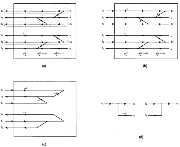
Given a pre-specified system represented as an interconnection of functions and a pair of terminal variables whose input-output configurations we wish to exchange, a convenient way of obtaining a behaviorally-equivalent system will specifically be to identify a functional path from the unmodified input to the unmodified output, and refer to this as the interconnecting system. Then the inputs and outputs to the interconnecting system are the overall input and output whose configurations we wish to exchange, in addition to the internal inputs and outputs connected to the functional path. The desired system can likewise be obtained by creating a behaviorally-equivalent path where the overall input and output configurations have been exchanged and the internal input and output configurations remain unmodified, using, e.g. the straightforward rules depicted in Fig. 2-7.

An example of the use of these rules in inverting the nonlinear system as discussed in [4, 7) is illustrated in Fig. 2-8. Referring to this figure, the elements along the

outlined path in Fig. 2-8(a) are replaced with the behaviorally-equivalent elements depicted in Fig. 2-7, resulting in the inverse system in Fig. 2-8(b).

(a)

(b)

NUM DEN

Figure 2-7: (a) Elements along a functionally-dependent path from an input to an out-put whose configurations are to be exchanged. (b) Behaviorally-equivalent elements that reverse the path.

(a)

(b)

c'[n] d'[n]

Figure 2-8: (a) Nonlinear system illustrating the functional path, or interconnecting system, from c[n] to d[n] that is used in exchanging the input-output configurations of these variables. (b) Behaviorally-equivalent system obtained by performing path reversal in the interconnecting system.

2.5

Partial taxonomy of 2-input, 2-output linear

systems

On a number of occasions related to viewing conservation principles under a change

of basis, we will be interested in implementing a linear transformation of the behavior

of a set of variables in a larger system. A specific sub-class of these transformations

that we will commonly encounter will be those corresponding to linear transformations

from R2 to R2. As the pertinent variables in the original system may be represented

in a number of possible input-output configurations, applying an appropriate

trans-formation generally involves realizing the pertinent behavior in a system that has a

compatible input-output configuration.

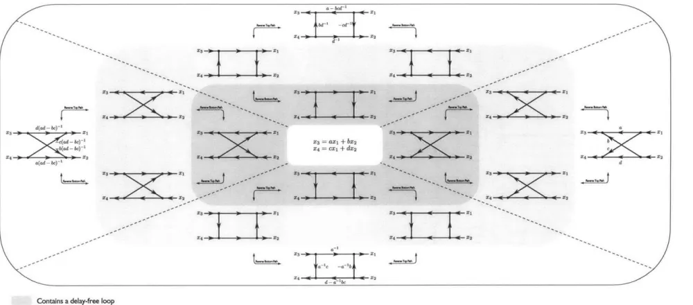
Toward these ends, Fig. 2-9 depicts a partial taxonomy of behaviorally-equivalent

linear signal-flow graphs that implement the linear transformation

X3 -

ax

+

(2.40)

X4 =

c

+

Referring to this figure, the signal-flow graphs were generated by beginning with

various implementations for the transformation specified in Eqns. 2.40-2.41, taking

x

and x

as inputs and x

and x

as outputs, and performing path reversal to realize

the depicted systems. The bent arrows in the figure indicate these manipulations.

Still referring to this figure, interconnections along upper-right, lower-left diagonals

have equivalent bottom branch configurations, and interconnections along upper-left,

lower-right diagonals have equivalent upper branch configurations.

Id-X3 1 d(ad -bc)-1 X3 1 42-3 :rz X, 3

z'zr:

zT

0

1M

:zizr:-

X

Contains a delay-free loop

Has multiple paths from an input to an output Has exactly one path from every input to every output

Figure 2-9: Partial taxonomy of behaviorally-equivalent 2-input, 2-output, linear, memoryless interconnections. The white

region contains interconnections in four input-output configurations, and the bent arrows indicate manipulations that can be

made by reversing the upper and lower input-output paths. Branch gains for the interconnections in the two gray regions may

be obtained using path reversal and are omitted here for clarity. Interconnections along upper-right, lower-left diagonals have

equivalent bottom branch configurations, and interconnections along upper-left, lower-right diagonals have equivalent upper

branch configurations.

X3 M 1

d

X 3 XI

Chapter 3

Conservation framework

As was previously mentioned, we are concerned in this thesis with conservation laws reminiscent of Eq. 1.1, with the general motivating problems being

e the design of signal processing algorithms for which a conservation law of the form of Eq. 1.1 is obeyed,

e the identification of conservation laws of the form of Eq. 1.1 in existing signal processing algorithms, and

e the role of these conservation laws in obtaining new and useful results.

Toward these ends, we focus in this chapter on gaining further insight into the fun-damental principles of conservation laws that take the form of Eq. 1.1.

In particular, we explore the question of what properties the left-hand side of Eq. 1.1 has, in addition to that of what causes the right-hand side of Eq. 1.1 evaluate to zero, laying much of the groundwork needed to address the remaining issues regarding the synthesis, identification, and use of conservation in signal processing algorithms. The details uncovered in doing so will in turn form a foundation for the remainder of the thesis. As the principles developed in this chapter will apply in a number of essentially unrelated applications, they will be viewed as a unifying framework within which to discuss conservation in signal processing systems.

A common theme in the remainder of the thesis will be that conservation is a prop-erty of a linear interconnecting system, and the results in this chapter form a very

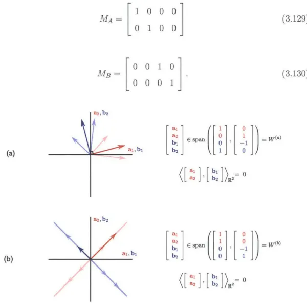
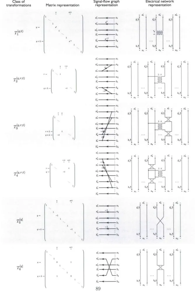
general foundation for applications such as this. We begin the chapter by formalizing the pertinent notion of conservation, introducing what we will refer to as an organized variable space (OVS) and illustrating its use by describing known conservation princi-ples in existing classes of signal processing algorithms. In cases where conservation is a result of variables lying in a vector space, we draw a distinction between whether an equation of the form of Eq. 1.1 corresponds to pairwise orthogonality of vectors or to orthogonality of vector subspaces, and we present a theorem establishing conditions on which this distinction may equivalently be based. We conclude the chapter by showing that the set of all conservative vector spaces forms a smooth manifold, in the process writing the generating set of matrices for the Lie group that can be used to move between them.

3.1

Organized variable spaces

In physical systems where conservation laws of the form of Eq. 1.1 hold, the corre-sponding conjugate variables may represent two of a wide range of different quantities. In these systems, a natural way to define conjugate variables in turn often involves identifying variables that can generically be thought of as efforts and flows. In signal processing systems, however, the system variables may be unitless or may have no par-ticular physical meaning. Although an effort-flow classification may still be effective in certain cases, e.g. for signal processing systems that simulate electrical networks or that move along continuous trajectories as in [21], it ultimately has the potential to lead to misguided or ambiguous concepts. For example, describing a quantity as a flow implies that something has been differentiated with respect to time, a notion that may require further clarification within the context of a discrete-time system. The concept of conjugate variables in this thesis therefore explicitly does not make use of this type of distinction.

A natural question, then, is that of how we might expect to identify candidate

variables that may potentially result in a conservation principle of the form of Eq. 1.1. This thesis takes the viewpoint that the critical issue is not what the variables

rep-resent, but rather the way that they are organized in giving rise to an expression akin to the left-hand side of Eq. 1.1, and that the behavior of the underlying signal processing system is what leads to the right-hand side of the equation evaluating to zero. These ideas are formalized in this thesis using an idea that we refer to as an

organized variable space (OVS).

3.1.1

The correspondence map

The central idea behind the OVS is to organize a collection of system variables, and to do so using the tools of linear algebra. The motivation behind the use of linear algebra is to allow conjugate variables to be defined as linear combinations of system variables, a property that will allow conservation in systems such as wave-digital filters to be placed on equal footing with conservation in, e.g., electrical networks. The interpretation will be that the values of the variables in a signal processing system can be thought of as coefficients in a basis expansion of a vector that lies in a finite-dimensional inner product space (V, (.,.)), defined over the real numbers, and that a quadratic form of a specific class can be used to map these coefficients to a real number. If the underlying signal processing system constrains its system variables so that the quadratic form evaluates to 0, the OVS will be said to be conservative for the behavior of the system.

A good reference for the basic principles in the theory of quadratic forms is [27],

and an attempt will be made in this thesis to formulate the key ideas in a way that does not require such a reference. One reason is that as the theory of quadratic forms is a rich topic in its own right, some of the accepted terminology in that field coincides with familiar concepts in inner product spaces. For example, an "orthogonal decomposition of a vector space" in the theory of quadratic forms does not generally have the usual inner-product space interpretation. Our approach will be to begin with an inner product space and use the inner product, in addition to a linear map, to define a quadratic form. This is indeed reminiscent of the usual progression in the theory of quadratic forms, where a bilinear form is first defined and is then used to create a quadratic form. However, the approach here in explicitly defining an inner

product will allow us to use the properties of inner products after the quadratic form has been defined, and to relate these back to the structure of the quadratic form in useful ways.

We will specifically be concerned with an even-dimensional inner product space

(V, (.,.)), where 2L = dimV > 2, in addition to an associated quadratic form

Q

V -+ R that is defined in terms of the inner product as

Q(X)

=

(Cx, x),

where C : V -> V is a linear map that will be assumed to be self-adjoint in this

definition without loss of generality, i.e. C* = C. The key restriction on C is that it

will be required to be invertible, with a total of L positive and L negative eigenvalues. The map C in this definition will be referred to as a correspondence map because in mapping V onto itself, it implicitly specifies a correspondence between any two vectors x, x' E V for which Cx = x'.

It is straightforward to verify that the quadratic form in the left-hand side of

'In this thesis, the adjoint of a linear map M V -- V on an inner product space (V, (.,.)) will

Eq. 1.1 has a valid correspondence map by writing it in the following way:

Q

/

/

,

with (.,.) denoting the standard inner product on R2K. In this equation, the matrix

C can be diagonalized as

C

S

-AS,

(3.3)