Compiling Array Computations
for the Fresh Breeze Parallel Processor
by
Igor Arkadiy Ginzburg
B.S. Computer Science and Engineering, Physics Massachusetts Institute of Technology, 2006
Submitted to the Department of Electrical Engineering and Computer Science in partial fulfillment of the requirements for the degree of
Master of Engineering in Electrical Engineering and Computer Science at the
MASSACHUSETTS INSTITUTE OF TECHNOLOGY
May 2007
)
M a s-c t
colg
©0 Massachusetts Institute of Technology 2007.
All rights reserved.Certified by ... Accepted by... MASSACHUSES INSTITUTE' OF TECHNOLOGY
OCT
0
3 2007
... .... .... . ..--Department of Electric IEngineeringidi Compircience
May 23, 2007
Jack Dennis -Professor Emeritus Th'sis, gpervisor
Arthur C. Smith Chairman, Department Committee on Graduate Students
Optimizing Array Manipulation
for the Fresh Breeze Parallel Processor
by
Igor Arkadiy Ginzburg
Submitted to the
Department of Electrical Engineering and Computer Science May 18, 2007
In partial fulfillment of the requirements for the degree of
Master of Engineering in Electrical Engineering and Computer Science
Abstract
Fresh Breeze is a highly parallel architecture currently under development, which strives to provide high performance scientific computing with simple programmability. The architecture provides for multithreaded determinate execution with a write-once shared memory system. In particular, Fresh Breeze data structures must be constructed from directed acyclic graphs of immutable fixed-size chunks of memory, rather than laid out in a mutable linear memory. While this model is well suited for executing functional programs, the goal of this thesis is to see if conventional programs can be efficiently compiled for this novel memory system and parallelization model, focusing specifically on array-based linear algebra computations. We compile a subset of Java, targeting the Fresh Breeze instruction set. The compiler, using a static data-flow graph intermediate representation, performs analysis and transformations which reduce communication with the shared memory and identify opportunities for parallelization.
Thesis Supervisor: Professor Jack Dennis Title: Professor Emeritus
Acknowledgements
I would like to thank Professor Jack Dennis for his advice and guidance when choosing the topic and implementing this project, and for his invaluable help and feedback with this document. I would also like to thank the National Science Foundation for supporting this work. Thank you to my family for your continual support.
Table of Contents
1. Introduction ... 9
2. Background ... 11
2.1. Fresh Breeze Architecture... 11
2.2. W riting Softw are for Fresh Breeze... 12
2.3. Fresh Breeze Arrays... 13
2.4. Parallelizing Array Com putation... 14
3. Com piler D esign ... 18
3.1. Functional Subset of Java ... 19
3.2. Functional Java w ith Arrays ... 22
3.3. Flat Representation ... 24
3.4. Data Flow Graph Representation... 26
3.4.1. D ata Flow Graphs ... 26
3.4.2. Com pound N odes... 27
3.4.3. Concrete Representation... 30
4. Com piler Im plem entation... 34
4.1. Flattening Byte Code ... 34
4.2. Constructing D ata Flow Graphs... 36
4.3. Data Flow Graph Transform ations... 38
4.3.1. N orm alizing the Representation ... 39
4.3.1.1. D ead Input Ports ... 39
4.3.1.2. D ead Output Ports... 40
4.3.1.3. Copy Propagation... 40
4.3.1.4. U nnecessary Loop Ports ... 41
4.3.1.5. Subtraction ... 42
4.3.2. Standard Optim izing Transform ations... 42
4.3.2.1. Constant Folding and Propagation... 43
4.3.2.2. D ead Code... 45
4.3.2.3. Com m on Sub-Expressions... 45
4.3.2.4. ining... 46
4.3.3. Fresh Breeze-Specific Transform ations... 47
4.3.3.1. Induction N odes... 48
4.3.3.2. In-Order Traversals... 49
4.3.3.3. Array Aliasing... 51
4.3.3.4. Parallelization ... 53
4.3.3.5. A ssociative Accum ulations... 54
4.3.4. Transform ation Fram ew ork... 55
5. Analysis... 58
6. Future W ork... 60
6.1. Choosing Array Representation... 60
6.2. Implem enting Code Generation... 61
6.3. Register Allocation ... 61
7. Conclusion...63
Appendix A: Test Cases...64
A .1 M atrix M ultiplication... 64
A.2 Cholesky D ecom position... 70
List of Figures
Figure 1: Executing Parallelizable Loops... 15
Figure 2: Parallelizable Loops ... 16
Figure 3: Compiler Design... 19
Figure 4: Limitations of Final Keyword ... 21
Figure 5: Default Functional Java Constructor... 21
Figure 6: Procedure Violating Secure Arguments Principle... 22
Figure 7: Satisfying Secure Arguments Principle but relying on Array Mutation ... 23
Figure 8: Array Syntax using Static Library methods ... 23
Figure 9: Functional Java Array Syntax ... 24
Figure 10: Flat IR Class Hierarchy and Structure... 25
Figure 11: Averaging 3 Inputs ... 26
Figure 12: Interesting DFG... 26
Figure 13: Constructing 1-Element Array ... 27
Figure 14: Retrieving Last Array Element... 27
Figure 15: DFG for Absolute Value ... 28
Figure 16: Code for Absolute Value... 28
Figure 17: DFG with Switch Node ... 29
Figure 18: Code with Switch Statement ... 29
Figure 19: DFG with Loop Node... 29
Figure 20: Code with Control Loop... 29
Figure 21: Conceptual DFG... 31
Figure 22: Concrete DFG... 31
Figure 23: DFG Class Hierarchy and Structure... 32
Figure 24: Simplifying Control Flow by introducing Boolean Variables ... 37
Figure 25: Compound Node with Dead Input... 39
Figure 26: Dead Input Port Removed ... 39
Figure 27: Eliminating Unused Outputs to Eliminate Unused Inputs ... 40
Figure 28: Copy Propagation leading to Dead Output Port Elimination... 40
Figure 29: Unnecessary Loop Port ... 41
Figure 31: Constant Folding Constant Inputs ... 43
Figure 32: Partial Constant Folding... 43
Figure 33: Constant Folding Compound Nodes ... 44
Figure 34: Propagating a Constant into a Compound Node enables Constant Folding... 44
Figure 35: Constant Folding generating opportunities for Dead Code Elimination... 45
Figure 36: Common Sub-Expression Elimination... 45
Figure 37: Inlining leading to Constant Folding... 46
Figure 38: Loop Invariant Code Motion... 47
Figure 39: Using Induction Nodes... 48
Figure 40: Method with an in-order array traversal... 50
Figure 41: Array Traversal Node Creation... 50
Figure 42: Array Construction Node Creation... 51
Figure 43: Method with input and output array having the same name ... 52
Figure 44: Array Get/Set Separation enables the creation of Array Construction Nodes and Array T raversal N odes ... . 52
Figure 45: Accumulation Node Creation... 55
Figure 46: Transformation Framework... 57
Figure 47: Functional Java Source Code for Matrix Multiplication... 64
Figure 48: Compiler Output for Matrix Multiplication ... 65
Figure 49: Innermost For All Node ... 67
Figure 50: Middle For All Node ... 68
Figure 51: Data Flow Graph for Matrix Multiply Method ... 69
Figure 52: Functional Java Source Code for Cholesky Decomposition... 71
Figure 53: Compiler Output for Cholesky Decomposition... 73
Figure 54: Functional Java Source Code for In-Place FFT ... 75
1.
Introduction
While feature sizes on silicon processor chips continue to shrink, allowing continued growth in the number of transistors per chip, concerns over power consumption have slowed the growth in clock speeds. These trends suggest the creation of parallel systems. Exploiting parallelism is essential, but difficult due to concerns over programmability. Fresh Breeze is a new multi-processor architecture designed in light of these trends, promising greater
performance for scientific computing while improving programmability.
Computations involving multi-dimensional arrays are important in scientific
computation. In "The Landscape of Parallel Computing Research: A View from Berkeley", [2] identify 12 common patterns of computation that have wide applications and serve as
benchmarks for parallel architectures. Three of these, including Dense Linear Algebra, Sparse Linear Algebra, and Spectral Methods, are commonly expressed as operations on arrays. Traditional implementations of these algorithms may manipulate these arrays in place, and in general assume a mutable, linear memory model.
One key aspect of the Fresh Breeze architecture is a write-once shared memory system. In this model, all data structures, including arrays, are represented by directed acyclic graphs of immutable fixed-size chunks of memory. So, Fresh Breeze arrays are neither mutable nor linear.
The goal of this work is to reconcile these two observations, allowing array-intensive programs written in a syntax that assumes the traditional memory model, to be efficiently executed on a Fresh Breeze computer. To that end, we have created a Fresh Breeze compiler, which compiles a subset of Java to the Fresh Breeze instruction set. The compiler is structured in several phases, with the majority of the analysis and transformations being performed on
intermediate representations that are independent of the specifics of either Java or the Fresh Breeze instructions set. The first phase converts Java byte code to a flat 3-operand intermediate representation (IR), enforcing some limitations on possible Java expressions. The second phase constructs Static Data Flow Graphs from the flat IR. This Data Flow Graph Representation is inspired by the intermediate representation of the Sisal compiler [8], and serves as the basis for a series of transformations. These include transformations that normalize the representation, standard optimizing transformations common to most compilers, and Fresh Breeze specific transformations that introduce nodes that make it easier to produce efficient, parallel Fresh Breeze code. The final phase of the compiler, which is still under development, will generate Fresh Breeze machine code from the Data Flow Graphs. The main contribution of this work is the design of the special Data Flow Graph nodes which describe opportunities for parallelization, and the implementation of Fresh Breeze-specific transformations which introduce these special nodes.
The remainder of this thesis is organized in six chapters. Chapter 2 gives background information on the Fresh Breeze architecture, the structure of Fresh Breeze arrays, and a strategy for parallelizing the execution of computations on Fresh Breeze arrays. Chapter 3 describes the design of the compiler, specifying the supported subset of Java, and detailing the intermediate representations. Chapter 4 describes the implementation of the compiler, including the
construction of Data Flow Graphs, and the specific analysis and transformations that are applied to generate the special nodes. In Chapter 5 we evaluate the compiler's output on several
representative linear-algebra routines. In Chapter 6 we propose future extensions to the compiler and discuss their implementation. Finally, in Chapter 7 we discuss the general conclusions of this work.
2. Background
2.1. Fresh Breeze Architecture
Fresh Breeze is a multiprocessor chip architecture which uses the ever-increasing numbers of available transistors for parallelism rather than complexity. By using a RISC instruction set and a simplified pipeline, multiple Multithreaded Processors (MP) can be placed on one chip. To create even more powerful systems, multiple MP chips may be connected together to create a highly parallel system [3].
Fresh Breeze differs from conventional computer architectures in several ways. A global shared address space is used to simplify communication between processors, and eliminate the need for a separation between "memory" and the file system. The shared memory holds
immutable 128-byte chunks, each addressed by a 64-bit Unique Identifier (UID). Chunks can be created and read, but not modified once created. This eliminates the cache-coherence problems that can add complexity to traditional multi-processor designs. A reference-count based garbage collector, implemented in hardware, is used to reclaim unused chunks, freeing the associated UIDs. This mechanism can be very efficient, but requires the heap to be cycle-free.
The Fresh Breeze instruction set facilitates the creation and use of these chunks. A ChunkCreate instruction allocates a new chunk returning its UID. New chunks are considered unsealed, meaning that they are mutable, and can be updated using the ChunkSet instruction. To prevent the formation of heap cycles, the ChunkSet instruction cannot place the UID of an unsealed chunk into another unsealed chunk. A chunk can be sealed, or made immutable, by a ChunkSeal instruction. Directed Acyclic Graphs (DAGs) of chunks can be created by placing UIDs of sealed chunks into newly-created unsealed chunks using the ChunkSet instruction. Data
structures in Fresh Breeze programs are represented using these chunk DAGs. Arithmetic operations cannot be performed on ULDs, preventing functions from accessing chunks that where not passed in as parameters and aren't reachable from pointers in the parameter chunks. Chunk data can be read using the ChunkGet instruction. Both the ChunkGet and ChunkSet instructions provide for bulk memory transfers by operating on a range of registers, rather than being
restricted to moving one word at a time.
This memory architecture allows for a novel model of execution, which provides for simultaneous multithreading while guaranteeing determinate behavior. The immutable nature of the memory guarantees that functions cannot modify their parameters, preventing them from
exhibiting side-effects. This enforces the secure-arguments principle of modular programming and eliminates race conditions, the major source of non-determinacy in traditional parallel
computation. Basic parallelism is achieved through a Spawn instruction, which starts the
execution of a slave thread, passing it some parameters, and leaving a "join ticket" as a handle on that thread. UIDs of unsealed chunks cannot be passed as parameters through Spawn calls, preventing multiple threads from modifying the same chunk. When the slave thread completes
its computation it returns a value using the EnterJoinResult instruction. The master thread can issue a ReadJoinResult instruction to retrieve the value returned by the slave. If the slave has not finished, the ReadJoinResult instruction stalls until the slave thread is done. By issuing several Spawn instructions before reading the join results, multiple parallel slave threads can be
instantiated. Other forms of parallelism, such as producer/consumer parallelism, as well as explicitly non-determinate computations are also supported [4], but are not relevant to the present work.
Software written for a Fresh Breeze system must be able to utilize the massive parallelism provided by the architecture, without creating cycles in the shared memory or mutating existing chunks. These requirements are met by functional programming languages. Purely functional programs do not allow mutation of data, and are therefore easy to parallelize, without creating race conditions or cycles in memory. Functional procedures create new output
data based on some input data, rather than updating the input data in place.
Although many functional languages exist, they have some drawbacks. Most, in an effort to support "stateful" programming, are biased towards execution on a sequential computer.
Others, like Val [7] and Sisal [6] have no available working front ends. Additionally, our main goal is to examine whether functional programs written within the constraints of a popular syntax, which assumes the standard linear, mutable memory model, can be efficiently compiled for Fresh Breeze. Therefore, the Fresh Breeze compiler is written to translate a new functional language, based on the Java language, called Functional Java.
Java is attractive for several reasons. Its primitive types are well suited for the Fresh Breeze RISC architecture. Its strong type system is helpful both for writing modular code, and for creating program graph models of that code. In addition, Java has a popular syntax, derived from C, and existing compilers and development environments. By using a language which is compatible with existing Java compilers, we avoid the task of building a compiler front end. 2.3. Fresh Breeze Arrays
Arrays are data structures mapping indices to values. On a conventional architecture with a linear, mutable memory, an array with n t-byte elements is usually represented by a contiguous region of n * t bytes in memory, starting at some memory address 1. The value at index i can be read or written by manipulating the t bytes at memory address 1+ i * t. This representation
affords fixed size, mutable arrays, matching the properties of Java's built in array class. Java arrays are intended to be implemented as a contiguous sequence of memory cells, providing constant time reads and writes to individual elements.
This representation is not possible on a Fresh Breeze system, where data is stored in chunks whose addresses are not subject to arithmetic operations. Fresh Breeze arrays, like all other Fresh Breeze data structures, must be represented as directed acyclic graphs of chunks. In
[3], a representation of Fresh Breeze arrays as fixed depth trees is proposed, where the elements
are stored in leaf chunks, and the order of the elements is specified by an in-order traversal of the tree.
An array with n 16-byte elements can be represented by a tree of depth k = floor(logl6n). While an individual element can be read in such an array (by traversing k chunks), its value cannot be mutated. Changing a value requires creating k new chunks, and produces a new array. The main challenge of the Fresh Breeze compiler is to achieve good performance in light of these properties.
2.4. Parallelizing Array Computation
In order to achieve good performance, we need to take advantage of the parallelism available on Fresh Breeze. This can be done by partitioning computation among different threads. Computations involving arrays are often performed in loops that read through existing arrays or construct new ones. If we can assign different iterations of a loop to different threads, we can greatly reduce computation time.
While not all loops in a Java program can be parallelized, many parallelizable loops are fairly easy to identify. In one such class of loops, each iteration computes a set of values which do not depend on the results of previous iterations, and then the values are combined to produce
the loop's outputs. These values can be combined as elements of a new array, or accumulated to produce a scalar result.
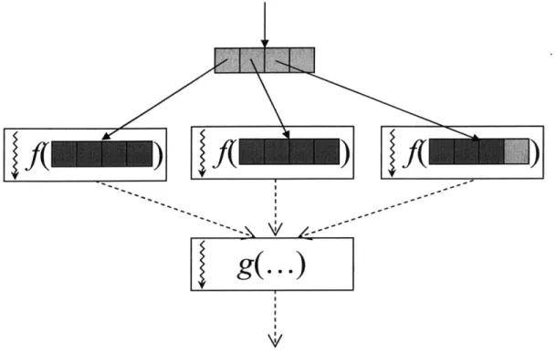
Figure 1: Executing Parallelizable Loops
Our plan for parallelization utilizes the Fresh Breeze primitives discussed in Section 2.1., and is depicted in Figure 1. When encountering a parallelizable loop, a master thread will partition the loop's iterations into a set of intervals, and issue a series of Spawn instructions creating a slave thread for each interval. Each slave thread will be passed its interval, and the inputs to the loop. If a slave thread will only need a subset of an input array's elements, then it can just be passed a sub-tree of the array, possibly just one leaf chunk, containing those
elements. The slave will then compute a set of output values. If the loop is constructing an array, then the slave's output will include a sub-tree of the array, or even just one leaf chunk of the array, depending on the granularity of the parallelization. The slave will place the output values on a chunk, and issue an EnterJoinResult instruction with the UID of that chunk. If there
is only one output value, then the slave can just enter that value directly. These computations by the slave threads are identified by the functionf in Figure 1.
After issuing all the Spawn instructions, the master thread will then retrieve the values computed by the slave threads by issuing a series of ReadJoinResult instructions. For scalar outputs, the master thread will use the corresponding operator to accumulate each result. For array outputs, the thread will build up an array tree out of the sub-trees returned by the slave threads. This computation by the master thread is denoted by the function g in Figure 1.
This parallelization plan has several consequences. First, the operators used to combine scalar values into a scalar output must be associative and commutative, to guarantee correctness when iterations are partitioned among slave threads. This is a general parallelization requirement not specific to Fresh Breeze. Second, when an output is a new array, the loop's iterations must produce the array elements in order, either first to last or last to first. Otherwise, the sub-trees returned by the slave threads might have overlapping index ranges, and the master thread will not be able to easily combine these overlapping sub-trees into a tree for the final array. In the
standard mutable memory model, this requirement can be relaxed to specifying that each array element is set by exactly one iteration, but they can be set in any order.
public static double dotProduct (double [ ] a, double[] b)
double sum = 0;
for (int i = 0; i < a.length; i++) {
sum += a[i] * b[i);
return sum;
public static double[] arraySum(double a[], double[] b)
double[] c = new double[a.length];
for (int i = 0; i < a.length; i++) {
c[i] = a[i] + b[i];
}
return c;
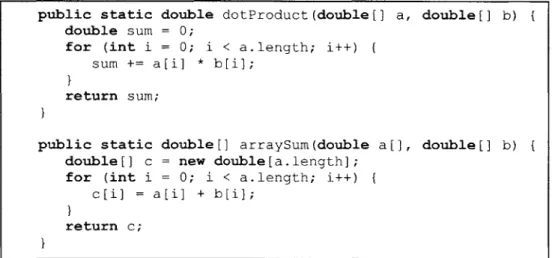
In Figure 2 we see two examples of loops that meet these requirements. In the
dotProducto example, the loop takes in two arrays and outputs a scalar value. The values can be
combined using double-precision floating point addition. While this operation is not strictly associative due to rounding errors, for any particular grouping it guarantees a consistent,
repeatable result. This is sufficient for us to treat float point addition like an associative operator.
If we describe the execution of dotProductO in terms of Figure 1, the functionf computed by
each slave thread would be a dot product of the vectors defined by a subinterval of the array indices. The function g computed by the master thread would be the summation of the values returned by the slaves.
In the arraySumO example a new array is constructed by adding the corresponding elements of two input arrays. Here, the slaves threads would be handed sub-trees of the input arrays, a and b. They would each construct and return the corresponding sub-tree of the output array, c. The master thread would then combine the returned sub-trees into a full tree to represent the output array.
In this discussion we have limited ourselves to the parallelization primitives described in Section 2.1. Fresh Breeze may also support additional kinds of spawn and join instructions which perform the associative accumulations or array constructions directly in hardware. Having the master thread issue one of these instructions, rather than a multiplicity of Spawns
followed by a series of ReadJoinResults, may greatly improve performance.
Specific details on how the compiler identifies and represents these parallelizable loops are found in Section 4.3.3, which describes the Fresh Breeze-specific analyses and
3. Compiler Design
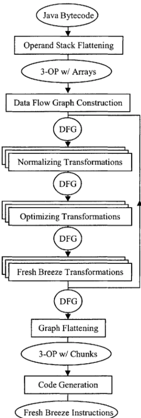
The compiler is designed such that the majority of the work is independent of the specifics of Java Bytecode and the Fresh Breeze instruction set, and will therefore be useful in other settings. To that end, the compiler consists of several phases which operate on different intermediate representations. The initial input is Java Bytecode, which can be generated using an existing Java compiler. In the first phase, the Bytecode is checked to satisfy the requirements of Functional Java and converted to a 3-Operand flat intermediate representation with explicit array manipulations operations. In the next phase Static Data Flow Graphs are constructed from the 3-Operand IR. The Data Flow Graph Representation is then subject to a series of analysis and transformations, including transformations that normalize the representation, standard optimizing transformations common to many compilers, and Fresh Breeze specific transformations that introduce nodes that make it easier to produce efficient, parallel Fresh Breeze code. These transformations are repeated until a fixed point is reached. The following phase flattens the Data Flow Graphs, producing a 3-Operand representation which manipulates chunks rather than arrays. Finally, in the last phase, Fresh Breeze instructions are generated from the 3-Operand representation. This structure can be seen in Figure 3.
Operand Stack Flattening
3-OP w/ Arrays
Data Flow Graph Construction
DFG Normalizing Transformations DFG Optimireze Transformations Graph Flattening 3-OP w/ Chunks Code Generation
Figure 3: Compiler Design
The remainder of this chapter describes the compiler's input language and intermediate representations. These include the Functional Java language, the 3-Operand Flat Representation, and the Data Flow Graph Representation.
Due to the reliance on existing Java compilers, Functional Java must be a subset of Java. In particular, it should be described by a set of rules stating which existing Java expressions are allowed and which are not. To give a better understanding of the constraints imposed by the Fresh Breeze memory architecture, we describe in this section a specification for Functional Java which includes Object types, even though our present compiler implementation does not allow their use.
The main requirements placed on Functional Java are that the generated code cannot mutate sealed Chunks or create reference cycles of Chunks. We will make several assumptions about how the generated code maps Java fields and Objects to Fresh Breeze memory structures. First, each Java object will reside on one or more Chunks. So, any Java object reference can be considered a reference to a Chunk. Additionally, any other globally accessible data will also reside on Chunks. These assumptions, when combined with the stated requirements, imply some general rules about Functional Java. First, all Object fields, of both reference and primitive type must be immutable, since they reside on immutable chunks. Similarly, static fields must also be immutable. Furthermore, it should not be possible to create reference cycles between Objects or allow Objects to contain a self-references, since this will create reference cycles in the shared memory. While a purely functional language may also require local variables to be immutable, this is not required to make Functional Java implementable on Fresh Breeze.
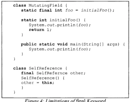
Java'sfinal keyword can be used enforce the immutability of both object fields and static fields. However, this alone does not prevent the formation of reference cycles and even some mutations. This is because a constructor can reference the generated object before setting its fields, and static field initializers can access the field before initializing its value. The code in
mutates a staticfinal field, and the class SelfReference which creates a self-reference using a final field.
class MutatingField
static final int foo = initialFoo();
static int initialFoo() {
System.out.println(foo); return 1;
public static void main(String[] args) System.out.println(foo);
class SelfReference
final SelfRefernce other; SelfReference()
other = this;
Figure 4: Limitations of final Keyword
To overcome these two limitations we impose additional constraints on Functional Java programs. First, we require that static fields are assigned solely constant (literal) values. Second, we enforce a default form for the constructor where each field value is passed in as a parameter. So, a class with N fields would have a constructor of the form shown in Figure 5.
Constructor(Typel fieldl, Type2 field2, ... , TypeN fieldN) {
this.fieldl = fieldl;
this.field2 = field2;
this.fieldN = fieldN;
Figure 5: Default Functional Java Constructor
The Java API is integrated with the language. For example, a large portion of the API can be reached by following the methods ofjava. lang. Object. The specifications of many of the Java API classes do not conform with the Functional Java requirements and would be difficult if not impossible to implement on Fresh Breeze. So, a separate designed Fresh Breeze API would be necessary to support a Fresh Breeze compiler which allowed for object types.
3.2. Functional Java with Arrays
Since this work is focused on compiling array manipulations, we ignore the aspects of Functional Java that deal with object types, and instead focus on arrays. Without object types, we are limited to a language which contains static methods, primitive types, and
multidimensional arrays of primitives. Fortunately these constructs are sufficient for expressing the types of computations that we wish to compile (Linear Algebra and Spectral Methods).
Now, since Fresh Breeze arrays are immutable, it may be difficult to generate code from programs that contain arbitrary Java array manipulations. For example, in the Java procedure in
Figure 6 an array is passed in as an argument and then mutated. Generating Fresh Breeze code
for this procedure while maintaining the semantics of Java would not be possible, since the chunks containing the array cannot be mutated.
void bad negate(int[ a) {
for (int i = 0; i < a.length; i++)
a[i] = -a[i];
Figure 6: Procedure Violating Secure Arguments Principle
By mutating its arguments the above procedure violates the Secure Arguments principle
of modular programming [3]. Such procedures can be prohibited from Functional Java, although in some cases, due to aliasing, additional analysis may be required to determine if a procedure is actually modifying its arguments. But, even if this restriction were enforced, it may not be sufficient to ensure simple code generation. Figure 7 contains a procedure that does not violate the Secure Arguments principle, but still makes Fresh Breeze code generation difficult.
int[] example(boolean x)
int a[] = new int[1l;
int b[] = new int[l];
if (x) I
a = b; a[0] = 1;
return b;
Figure 7: Satisfying Secure Arguments Principle but relying on Array Mutation By copying array references, the procedure makes it difficult to determine at code
generation which array references are affected by an assignment to an array element. One way to avoid this problem is to preclude array reference re-assignment, statements of the form "a =
b;" where a and b are arrays. This would be equivalent to marking all array declarations "final".
An alternative would be to allow array reference re-assignment, but disallow array element assignments, or statements of the form "a[i] = x;". Then Functional Java arrays would truly be immutable, closely matching the underlying Fresh Breeze arrays. A static library method would be provided for creating new arrays based on existing ones. Figure 8 contains a trivial example which exercises this syntax:
boolean alwaysTrue ()
long[] a = new long[10];
a = FBArray.set(a, a.length-1, 5);
return a[9] == 5;
}
Figure 8: Array Syntax using Static Library methods
While explicit in its interpretation and closely related to the underlying representation, the syntax in Figure 8 would be unfamiliar and awkward to programmers. So, we simplify array syntax by reinterpreting array element assignments to include a reassignment of the array
reference. This reinterpretation also resolves the parameter problem we exposed in Figure 6, since without mutation arrays are in essence passed by value.
int[] negate(int[] a) {
for (int i = 0; i < a.length; i++) {
a[i] -a[i];
return a;
}
Figure 9: Functional Java Array Syntax
While reinterpreting the meaning of array-element assignment preserves the general style of the code, in some cases it can make Functional Java execution inconsistent with Java. It should be possible to create an analyzer which statically determines if a particular program may give different results when interpreted as Functional Java rather than Java, and reject such programs from compilation. We did not implement such an analysis, leaving it up to the programmer to determine if the code is correct under the Functional Java interpretation of array element assignment. Designing such an analysis is an interesting avenue for future work. In practice, this array syntax and semantics worked well when implementing the tests and
benchmarks for the compiler. Figure 9 demonstrates how array negation may be written using the Functional Java array syntax.
3.3. Flat Representation
We use a generic flat representation of Functional Java methods to separate our work
from the specifics of both Java Bytecode and the Fresh Breeze instruction set. This makes the compiler more general and useful, making it possible to add support for additional source language feature or accommodate changes to the Fresh Breeze instruction set with minimal changes to the compiler. Additionally, by abstracting away irrelevant aspects of the source and destination languages, such as Bytecode's operand stack or Fresh Breeze's register layout, we can simplify the Data Flow Graph Construction and Graph Flattening phases of the compiler.
The Flat IR is a three operand representation, with statements that contain two input operands and 1 output operand. This matches Fresh Breeze's RISC instruction set, where most
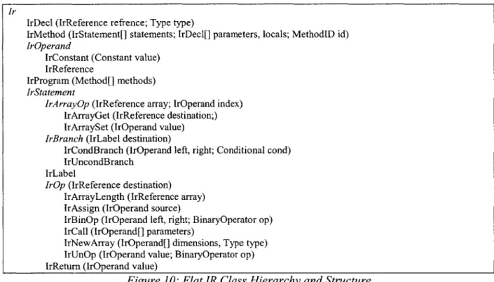
instructions generally have two sources and one destination register. The operands can be constant values or references to local variables. Local variables are typed, with types corresponding to the arithmetic types supported by Fresh Breeze (Int, Long, Float, Double). When constructed from Bytecode the Flat IR can contain Array types. The type of an array's elements is not included in the array's type information, but rather specified by the statements that construct and access arrays. Similarly, before being used to generate Fresh Breeze instructions, the Flat IR can contain Chunk types, whose sealed or unsealed status can be specified in the Type information.
Ir
IrDecl (IrReference refrence; Type type)
IrMethod (IrStatement[] statements; IrDecl[] parameters, locals; MethodlD id)
IrOperand
IrConstant (Constant value) IrReference
IrProgram (Method[] methods)
IrStatement
IrArrayOp (IrReference array; IrOperand index)
IrArrayGet (IrReference destination;) IrArraySet (IrOperand value)
IrBranch (IrLabel destination)
IrCondBranch (IrOperand left, right; Conditional cond) IrUncondBranch
IrLabel
IrOp (IrReference destination)
IrArrayLength (IrReference array) IrAssign (IrOperand source)
IrBinOp (IrOperand left, right; BinaryOperator op) IrCall (IrOperand[] parameters)
IrNewArray (IrOperand[] dimensions, Type type) IrUnOp (IrOperand value; BinaryOperator op) IrReturn (IrOperand value)
Figure 10: Flat IR Class Hierarchy and Structure
Figure 10 depicts the class hierarchy of the Flat IR. A program consists of a list of
methods. Each method is uniquely identified by package, class, name, parameter types, and return type. A method contains an ordered list of statements, and defines the types of its parameters and local variables. The statements take in operands, which are either constants or reference to temporaries. While most statements take in two operands, some like method calls
have a variable number of operands. Control flow is facilitated by branch statements that point to label statements. Conditional branches take two input operands and specify a comparison operator. The Flat IR is immutable and implements the visitor design pattern [5] to facilitate traversal.
3.4. Data Flow Graph Representation
The bulk of the analysis and transformations performed by the compiler are done on a Data Flow Graph Representation. This representation makes data dependencies explicit, simplifying many analyses. Data Flow Graphs assume that functions produce new output data from input data without mutation, complementing the Fresh Breeze memory model. This representation is inspired by the intermediate representation used in the Sisal compiler [8].
3.4.1. Data Flow Graphs
A Data Flow Graph is a labeled directed acyclic graph. The edges carry values, and the
nodes are labeled by functions which take in values from their incoming edges and compute new values for the outgoing edges. A set of edges are designated as input edges, and correspond to the inputs of the graph. Similarly, a different set of edges corresponds to the outputs.
Figure 11: Averaging 3 Inputs Figure 12: Interesting DFG
Figure 11 depicts a Data Flow Graph which computes the average of three numbers. The graph contains three input edges and one output edge. The inputs are summed using two-input
+ 3
addition nodes and then divided by three, a value produced by a no-input constant node. In general, Data Flow Graphs can have arbitrary numbers of inputs and outputs and the value computed by a single node can be used in multiple places. Values can also be carried from the graph's inputs to outputs directly, bypassing any intermediate nodes. Figure 12 depicts these possibilities.
0 [].length
new[] -1
Figure 13: Constructing 1-Element Array Figure 14: Retrieving Last Array Element In addition to computing standard arithmetic operations, Data Flow Graphs can represent operations on arrays. We utilize four kinds of nodes that operate on arrays: creating a new array given the size as input, outputting the length of an array, getting the value of an element at a particular index, and constructing a new array from an existing one by changing the value of one element at a given index. These nodes are shown in Figure 13 which depicts a graph that outputs a new one-element array containing the value "-1", and in Figure 14 with a graph that retrieves the last element of an input array. We use heavy lines for edges that contain array pointers.
3.4.2. Compound Nodes
In the Data Flow Graphs presented so far, each node is evaluated exactly once, corresponding to straight line code within a program. To represent computation with control
flow, we introduce compound nodes. These nodes contain, as part of their labeling, internal Data
Different kinds of compound nodes have different rules for which internal graph is evaluated and how values are passed into and out of that graph, allowing for conditionals, loops and other kinds of control flow. int abs(int x) if (x < 0){ return -x; } else { T F return x;
Figure 15: DFGfor Absolute Value Figure 16: Code for Absolute Value In general, the graphs within a compound node contain identical sets of input edges and identical sets output edges, both in number and type. The inputs to the node flow as inputs to the
graphs, and the outputs of the graphs flow as outputs of the node. A Conditional node is a kind of compound node that can be used to represent simple if/else statements. It contains two graphs, one for the true case and one for the false case. The node has two special inputs which do not
flow into its graphs, but are compared using a conditional operator to determine which graph gets evaluated. Figure 15 contains an example of a conditional node which computes absolute value (the corresponding Java code is shown in Figure 16). The node contains two input, one-output data flow graphs, one which negates its input and one which does not. The node has three inputs, two of which are compared using the "less than" operator, and one which is passed into both graphs. It has one output which is chosen from the graph corresponding to the result of the
int fibonacci (int x) switch (x) { case 0: return 0; case 1: case 2: return 1; case 3: return 2; V V V V V case 4: return 3; 0{} {1,2} {3} {4} {5}; case 5: return 5;
Figure 17: DFG with Switch Node Figure 18: Code with Switch Statement
While Conditional nodes are sufficient for representing any computation which does not contain loops in the control flow, other kinds of compound nodes can represent that computation more directly, making it simpler to generate quality code. A switch node is one such compound node that can be used to better represent Java switch statements. Each of a switch node's sub-graphs is associated with a disjoint set of integers, and the node takes one special input, an integer which selects the graph that is evaluated. Figure 17 contains a switch node which evaluates the first few terms of the Fibonacci sequence, and corresponds to the code in Figure
18. 1 int count(int x) int i = 0; do = + 1 } while (i <= x); return i;
Figure 19: DFG with Loop Node Figure 20: Code with Control Loop
In order to represent loops in control flow we need a different kind of compound node. A Loop node corresponds closely to Java's do{}whileo statement. A loop node contains one sub-graph, which is reevaluated for each iteration of the loop. The sub-graph has two special outputs
which are compared with a conditional operator to determine loop terminations. Other sub-graph outputs, designated as loop edges, are fed back into the inputs for the next iteration. The sub graph can have additional inputs which are not designated as loop edges, whose values always flow from the loop node's inputs. For the first iteration values for the sub-graph's loop inputs flow from the node's inputs, and after the final iteration the sub-graph's loop outputs flow as the loop node's outputs. Figure 19 contains a Data Flow Graph with a loop node which corresponds to the simple do(}whileO statement in Figure 20.
Loop nodes and Conditional nodes are sufficient for representing the control flow of arbitrary Functional Java programs. Logical operators like ANDs and ORs can be constructed
by combining Conditional nodes tied with edges carrying boolean values. Other kinds of loop
statements, likeforo(){} and whileo(){}, can be simulated by wrapping a Loop node in a Conditional node to condition the first iteration.
3.4.3. Concrete Representation
The specific Data Flow Graph Representation used by the compiler is based on the conceptual Data Flow Graphs defined above. The representation uses special nodes to identify a graph's input and output edges. A Data Flow Graph contains an input-less Source Node whose outputs determine the inputs to the graph, and an output-less Sink Node whose inputs determine the outputs of the graph. This design decision makes it possible to write code which analyzes or transforms data flow graphs without including special cases for a graph's input and output edges.
The nodes within a Data Flow Graph are ordered such that the Source Node is first, the Sink Node is last, and other nodes appear after the nodes they depend on. This invariant simplifies both the analysis of the graphs, and the graph flattening phase. Additionally, this invariant guarantees that the graphs are acyclic. While the conceptual Data Flow Graph
drawings omit type information, nodes in the concrete Data Flow Graph representation specify the types of their output ports. By enforcing consistency of this type information across
compound nodes it is possible to sanity-check the correctness of a Data Flow Graph after a transformation.
The edge information is stored in Use-Def format, where each node contains a
description of its input edges. So in the concrete representation, unlike the conceptual drawings, edges point from the node that uses a value to the node that defines it. Both nodes and their output ports are numbers, such that the start of an edge in the graph can be specified by a pair of numbers, the node number and port number.
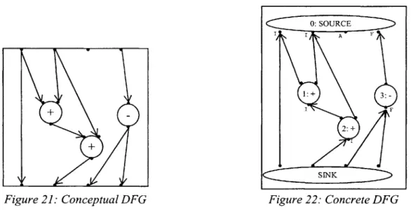
1:+ 3:
-+ _ F
2:+
Figure 21: Conceptual DFG Figure 22: Concrete DFG
The two figures above demonstrate the difference between the conceptual description of Data Flow Graphs and our concrete implementation. Figure 21 shows a sample conceptual Data Flow Graph, while Figure 22 show how it is represented by the compiler.
To maintain uniformity, compound nodes identify their special ports by specifying an input offset and an output offset. The input offset specifies a prefix of inputs that are not passed into the sub-graphs, while the output offset specifies a prefix of sink ports that are not passed from the sub-graphs to the compound node's output ports. So, for a Conditional node the input
offset is 2, for the two special inputs that are compared, and the output offset is 0. Similarly, for a Switch node the output offset is also 0, and the inputs offset is 1, for the integer input that selects the graph. The input offset for a loop node is 0 since all the inputs flow to the sub-graph, but the output offset is 2, for the two sink ports that are compared during each iteration. In addition to the input offset and output offset, loop nodes specify a loop port count identifying the number of sink edges whose values wrap around during each iteration of the loop.
Dfg
DfgGraph (DfgNode[] nodes)
DfgMethod (DfgGraph graph; MethodiD id) DfgProgram (DfgMethod[] methods)
DfgNode (Edge[] inEdges; Type[] outTypes)
DfgCompoundNode (DfgGraph[] graphs; int inputOffset, outputOffset)
DfgConditionalNode (Conditional cond)
DfgLoopNode (Conditional cond; int loopPortCount) DfgSwitchNode (Constant[][] cases)
DfgSimpleNode DfgArrayNode
DfgArrayGet DfgArrayLength DfgArraySet
DfgBinOpNode (BinaryOperator op) DfgConstantNode (Constant const) DfgMethodCall (MethodlD id) DfgNewArray (Type arrayType) DfgUnOpNode (UnaryOperator op) DfgGraph.SourceNode
DfgGraph.SinkNode Edge (int nodelndex, portlndex)
Figure 23: DFG Class Hierarchy and Structure
Figure 23 depicts the class hierarchy and structure of the Data Flow Graph
Representation. Like the Flat IR, a program consists of a list of named methods. A method contains a Data Flow Graph with a number of input edges corresponding to the method's parameters, and one output edge corresponding to the method's return value. A Data Flow Graph consists of a list of nodes, starting with a Source Node and ending with Sink Node. Each node has a list of incoming edges, each specified by a node index and a port index, and a list of output types. Simple nodes have one output port, while compound nodes contain a list of Data
Flow Graphs. The unary and binary operators, as well as conditionals, supported by the Data Flow Graph Representation are identical to those in the Flat IR. Data Flow Graphs and their nodes are immutable, and are traversed by dispatching on type using the instanceof operator.
The nodes listed in Figure 23 are sufficient for representing the structure of Functional Java programs. The compiler supports additional kinds of nodes which are created during the analysis and transformation phase. These additional nodes represent the information gathered by the analysis, and make it possible to generate improved Fresh Breeze code which better utilizes the Fresh Breeze memory model and takes advantage of the parallelism available in the Fresh Breeze architecture. These nodes are described in conjunction with their associated
4. Compiler Implementation
The goal of our compiler implementation is to demonstrate the feasibility of effectively compiling Functional Java for Fresh Breeze. While the implementation sets up a framework for a robust compiler, we focused our development efforts on the novel aspects of the compiler, specifically the non-standard transformations in the Data Flow Graph Transformation phase. More common phases, such as the Operand Stack Flattening and Data Flow Graph construction phases, have more skeletal implementation, which are sufficient for testing the Transformation phase, but are not necessarily robust or comprehensive enough for extensive use. Finally, the last few phases of the compiler, including the graph flattening and code generation phase have not been implement, and are described in Future Work (Chapter 6).
4.1. Flattening Byte Code
Rather than compiling Functional Java source files directly, we first use an existing Java compiler, such as Javac or the Eclipse Incremental Compiler, to generate Java class files. Class files contain Java Bytecode, a flat stack-based representation. The first phase of the compiler converts these Java class files into the 3-Operand Flat Intermediate Representation, while checking that the input confirms to the Functional Java specifications. This approach simplifies development effort, and provides compatibility for a wide range of Java language constructs.
The conversion from Bytecode to the Flat IR is based on previous work by Scott Beamer, who wrote a direct translator from Bytecode to Fresh Breeze instructions. Java Bytecode
assumes a fixed-sized array of local variables, and utilizes a stack of operands. Most Bytecode instructions pop their parameters from the operand stack, and push their output back onto the stack. Instructions are provided for moving operands to and from the local variable array and for
rearranging operands on the stack. Control flow is accomplished by branch instructions that specify the address of their destination. To simplify the conversion we assume that the operand stack is empty at the start and end of basic blocks. While this invariant is not required by the class file format, the assumption is mostly valid for Bytecode generated by Javac and the Eclipse Incremental Compiler. Without this assumption we would need to perform data-flow analysis on the Bytecode to determine the status of the operand stack.
Given the simplifying assumption, the conversion can proceed in one linear pass over the Bytecode. Each entry in the local variable table is assigned a temporary in the Flat IR, so a load or a store to a local variable becomes an access or an assignment to the temporary. The entries on the operand stack cannot be handled in the same way, since the same stack location can hold different data-types during execution. So, during the conversion, we statically simulate the stack contents, maintaining a stack of operands, which are either constants or references to temporaries in the Flat IR. While some Bytecode conditional branches specify the comparison operator, others rely on an earlier comparison instruction. Since the Flat IR does not have separate compare and branch instructions, we use static analysis to merge the separate Bytecode
instructions into one conditional branch. This requires allowing an additional kind of stack entry on our simulated operand stack, which stores the two operands of a comparison.
When converting a Bytecode instruction which loads a local variable onto the stack, either a reference to the variable's associated temporary can be pushed on the stack, or a new temporary can be pushed on the stack while an assignment to the new temporary is added to the generated Flat IR. If the local variable holds an array then creating a new temporary will change the meaning of the code, since the interpretation of array element assignments discussed in
not affect the value of the array in the local variable. On the other hand, there are several Bytecode instructions, such as iinc, which manipulate the values in the local variable table directly, bypassing the operand stack. If new temporaries are not created during loads, then these instructions will have the unintended consequence of changing the value of operands already pushed on the stack. Correct conversion is possible even in light of these contradicting observations, because none of the instructions that manipulate the local variable table directly operate on arrays. So, we create new temporaries only when loading primitive-typed local variables.
Our assumption about the contents of the operand stack at the end of basic blocks does
not hold in the case when Java's ternary operator (condition ? true Value :false Value) is
compiled. To deal with this special case, we create a new IR temporary for each such
conditional, maintaining a mapping from the Bytecode index where the two conditional cases merge to the associated temporary.
This implementation of the conversion from Bytecode to Flat IR meets ours goals. It is simple and reasonably efficient. The conversion is correct given that the Bytecode was
generated by the specific Java compiler it was designed for. While a more robust
implementation would be possible, and might at some point be added to the Fresh Breeze compiler, it is not necessary for this work, since the main focus of the thesis is on the Data Flow Graph Representation rather than the Flat Intermediate Representation.
4.2. Constructing Data Flow Graphs
The second phase of the compiler constructs Data Flow Graphs from the Flat
Intermediate Representation. After this point, the Flat IR is discarded and all transformations are done on the Data Flow Graph Representation directly. While the representation is general
enough to represent arbitrary computation, our goal was to develop a simple routine for converting most basic Functional Java programs.
boolean hasTrue(boolean[] [] bitMatrix)
for (int x = 0; x < bitMatrix.length; x++)
for (int y = 0; y < bitMatrix[x].iength; y++) {
if (bitMatrix[x][y]) {
return true;
return false;
boolean hasTrue equivalent(boolean[][] bitMatrix)
boolean returnFlag = false;;
for (int x = 0; !returnFlag && x < bitMatrix.length; x++)
for (int y = 0; !returnFlag && y < bitMatrix[x].length; y++)
if (bitMatrix[x][y])
returnFlag = true;
return returnFlag;
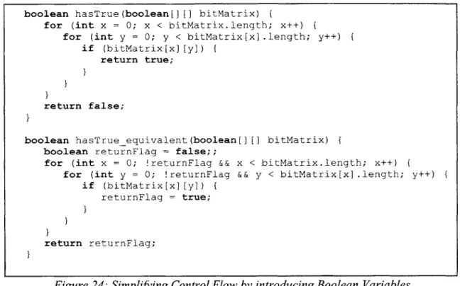
Figure 24: Simplifying Control Flow by introducing Boolean Variables
The conversion is similar to decompilation, since we are imposing structure on the control flow of low level instructions. But the conversion is more involved than just
decompilation, since some java constructs, such as return statements nested within loops, do not have strictly corresponding data flow graphs. Equivalent programs that do have directly
corresponding data flow graphs can be created by introducing additional boolean variables that carry information which is implicit in the original control flow. Figure 24 contains an example of such a Java method, has True, which iterates over a 2-dimensional array and has a return statement nested inside two loops. By introducing the returnFlag boolean variable we can convert hasTrue to an equivalent method which does not have this property. While this type of transformation is possible for all Functional Java constructs that do not have directly
constructs since they can be easily avoided. In addition to nested returns we don't handle nested continues or breaks, and compound logical operators. Future versions of the compiler may provide more complete support.
Data Flow Graph construction is implemented as a recursive procedure. The procedure takes in an index range over an array of Flat IR statements, and returns a Data Flow Graph corresponding to the statements within the range. The procedure fails if it encounters branch statements whose targets labels are outside of the range. A mapping is maintained from Flat IR temporaries to the Data Flow Graph edge that contains the temporary's current value. When control flow corresponding to an if(){}else{} statement is encountered, two recursive calls are made to construct a corresponding Conditional Node, one to generate each of the Conditional Node's sub-graphs. Similarly, when encountering a backwards branch corresponding to a Loop Node, a recursive call is made to generate a Data Flow Graph for the body of the loop. In both of these cases, it is assumed that any of the defined temporaries may be used by the recursive
calls, so the edges corresponding to all defined temporaries are given as inputs to the compound node under construction.
4.3. Data Flow Graph Transformations
In the third phase of the compiler a series of transformations are applied to the Data Flow Graph representation of the Functional Java program. Since the representation is immutable, each transformation creates a new program graph from a given program graph. There is a framework for applying the transformations, which cycles through a given set of transformations until a fixed point is reached and the program graph stops changing. The transformations are designed in such a way that a fix point will be reached for any input Functional Java program.
The compiler implements three kinds of transformations. Normalizing transformations reduce syntactic redundancy in the data flow graphs without changing their semantic meaning. Standard Optimizing transformations apply optimizations common to most compilers, improving the eventual performance of the generated code, and simplifying further analysis of the data flow graphs. Fresh Breeze-Specific Transformations identify opportunities for generating code which takes advantage of the Fresh Breeze memory model and model of execution, and introduce new kinds of nodes which describe these opportunities.
4.3.1. Normalizing the Representation
The Data Flow Graph representation defined in Section 3.4. allows for multiple representations of the same underlying computation. When performing analysis on Data Flow Graphs it may be useful to assume certain properties which are not guaranteed by the
specification of Data Flow Graphs. For example, it might be useful to assume that any value passed into a compound node is used within that node. The normalizing transformations
presented in this section provide these kinds of properties, by changing the syntactic structures of the graphs without affecting their semantic meaning.
4.3.1.1. Dead Input Ports
Figure 25: Compound Node with Dead Input Figure 26: Dead Input Port Removed The specification of Data Flow Graphs allows compound nodes to have inputs that are not used by any of their sub-graphs. In fact, the Data Flow Graph construction described in
Section 4.2. assumes that all available values are going to be needed, and generated compound nodes that take in every available edge. These unused, or dead, input ports generate unnecessary
dependencies in the Data Flow Graph, making further analysis of the graph less productive. The Dead Input Port Removal transformation identifies and removes input ports that are not used by any of a compound node's graphs. The transformation performs a traversal of each sub-graph to identify unused inputs. For Loop Nodes all loop ports are assumed to be used, or live, and are not removed by this transformation. Figure 25 shows a sample compound node with a dead input. Figure 26 has the node with the input removed.
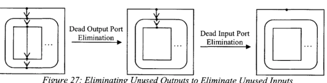
4.3.1.2. Dead Output Ports
Dead Output Port Dead Input Port
... Elimination Eliminatio.
Figure 27: Eliminating Unused Outputs to Eliminate Unused Inputs
In addition to unnecessary inputs, compound nodes can have unnecessary outputs. These are output ports that do not have any outgoing edges in the surrounding graph. Unnecessary, or dead, outputs can prevent the compiler from recognizing dead inputs, since the dead outputs preserve unnecessary edges in a compound node's sub-graphs. Figure 27 has an example of
such a compound node, where Dead Output Port Elimination is necessary, before Dead Input Port Elimination can proceed.
4.3.1.3. Copy Propagation
Dead Output Port
Copy Propagation Elimination
In traditional compilers, copy propagation replaced targets of direct assignments with their values. While Data Flow Graphs do not have assignment operators, and therefore don't need most types of copy propagation, there are circumstances under which a form of copy propagation can be applied. In particular, when an output from a compound is just a copy of one
of the inputs, we can bypass the compound node all together for that output value. This transformation is necessary because the Data Flow Graph Construction phase of the compiler passes all locals, even those that are not modified, through compound nodes. Figure 28 shows simple Data Flow Graph where Dead Output Port elimination cannot be performed without Copy Propagation. When combined with Dead Input Port elimination and Dead Output Port
elimination, Copy Propagation guarantees that inputs to compounds nodes are actually used within the nodes.
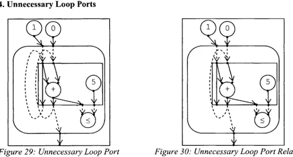
4.3.1.4. Unnecessary Loop Ports
5 5I
Figure 29: Unnecessary Loop Port Figure 30: Unnecessary Loop Port Relabeled Loop nodes specify a set of output ports whose values wrap around during each iteration of the loop. The Data Flow Graph construction phase conservatively labels all inputs to a Loop Node to be such loop ports. Many variables within a loop body do not change their value from one iteration to another, and therefore do not need to be labeled as loop ports. Unnecessary loop
ports stifle additional analysis and transformation, since they cannot be treated like normal inputs and outputs. For example, Dead Output Port elimination ignores loop ports, since their values may be reused within the Loop Node's sub-graph. The compiler identifies two types of unnecessary loop ports: those whose output value is a copy of the corresponding input value, and those whose output is a copy of input which is not a loop port. During Unnecessary Loop Port Elimination, the compiler removes the loop port label from input/output pairs that satisfy one of these conditions, leaving additional cleanup to the other normalizing transformations. The Loop Node in Figure 29 counts up from 0 to 5 in increments of 1, and contains an unnecessary loop port. The loop port is relabeled in Figure 30.
4.3.1.5. Subtraction
Another redundancy in the Data Flow Graph representation comes from the inclusion of both one-input negation operators and two-input subtraction operators. Excluding edge effects
and overflows, subtraction is equivalent to addition with one operand negated. So, the first transformation applied by the compiler is to replace all binary subtraction nodes with equivalent
combinations of binary addition and unary negation nodes. This transformation simplifies the implementation of subsequent analysis and transformation by reducing the number of binary operators. After all other transformations are complete, but before Data Flow Graph Flattening, the compiler reintroduces binary negation nodes, turning all additions where one of the operands
is negated into a subtraction. These simple transformations go a long way to simplifying the implementation of Constant Folding (Section 4.3.2.1), Induction Node Creation (Section 4.3.3.1.) and Accumulation Node Creation (Section 4.3.3.4.).