HAL Id: hal-01160579
https://hal.inria.fr/hal-01160579v2
Submitted on 3 Dec 2015
HAL is a multi-disciplinary open access
archive for the deposit and dissemination of
sci-entific research documents, whether they are
pub-lished or not. The documents may come from
teaching and research institutions in France or
abroad, or from public or private research centers.
L’archive ouverte pluridisciplinaire HAL, est
destinée au dépôt et à la diffusion de documents
scientifiques de niveau recherche, publiés ou non,
émanant des établissements d’enseignement et de
recherche français ou étrangers, des laboratoires
publics ou privés.
Polarised Intermediate Representation of Lambda
Calculus with Sums
Guillaume Munch-Maccagnoni, Gabriel Scherer
To cite this version:
Guillaume Munch-Maccagnoni, Gabriel Scherer. Polarised Intermediate Representation of Lambda
Calculus with Sums. Thirtieth Annual ACM/IEEE Symposium on Logic In Computer Science (LICS
2015), Jul 2015, Kyoto, Japan. �10.1109/LICS.2015.22�. �hal-01160579v2�
Polarised Intermediate Representation
of Lambda Calculus with Sums
Guillaume Munch-Maccagnoni
Computer Laboratory, University of Cambridge
Gabriel Scherer
Gallium, Inria Paris-Rocquencourt
Abstract—The theory of the 𝜆-calculus with extensional sums
is more complex than with only pairs and functions. We propose an untyped representation—an intermediate calculus—for the 𝜆-calculus with sums, based on the following principles: 1) Compu-tation is described as the reduction of pairs of an expression and a context; the context must be represented inside-out, 2) Operations are represented abstractly by their transition rule, 3) Positive and negative expressions are respectively eager and lazy; this polarity is an approximation of the type. We offer an introduction from the ground up to our approach, and we review the benefits.
A structure of alternating phases naturally emerges through the study of normal forms, offering a reconstruction of focusing. Considering further purity assumption, we obtain maximal
multi-focusing. As an application, we can deduce a syntax-directed
algorithm to decide the equivalence of normal forms in the simply-typed 𝜆-calculus with sums, and justify it with our intermediate calculus.
I. Introduction
The simply-typed 𝜆-calculus with extensional (or strong) sums, in equational form, is recalled in Figure1.
a) The rewriting theory of this calculus is more complex than with pairs and functions alone: As is well-known, the reduction relation on open terms requires additional commuta-tions, recalled in Figure2. But the complexity is also witnessed by the diversity of approaches to decide the 𝛽𝜂-equivalence of terms, proposed since 1995: based either on a non-immediate rewriting theory (Ghani [23]; Lindley [45]) or on normalisation by evaluation (Altenkirch, Dybjer, Hofmann, and Scott [3]; Balat, di Cosmo, and Fiore [6]).
Moreover, syntactic approaches are delicate, because there can be no 𝜆-calculus with sums à la Curry. Indeed, recall that cartesian closed categories with binary co-products and arbitrary fixed points are inconsistent (Lawvere [40]; Huwig and Poigné [33]). For the calculus in Figure1, this means that, in the absence of typing constraints, any two terms are equi-convertible (by a diagonal argument involving the fixed point of the function 𝜆𝑥.𝛿(𝑥, 𝑦.𝜄2(𝑦), 𝑦.𝜄1(𝑦)), see Dougherty [16] for
details).
b) On the side of proof theory: To begin with, sums become as simple as products once cast into Gentzen’s sequent calculus [22], perhaps because sequent calculus has an inherent symmetry that reflects the categorical duality between sums and products. For instance, commutations are not needed for reducing proofs. Thanks to abstract-machine-like calculi in the style of Curien and Herbelin [11], we can transfer the benefits of sequent calculus to term calculi.
The focusing discipline of proof theory provides a char-acterisation of cut-free, 𝜂-long proofs (Andreoli [4]). It has been applied to intuitionistic logic with sums by Liang and Miller [43, 44]. We continue the first author’s approach to focalisation [47], where the properties related to focusing are expressed as constraints to the reduction, rather than as restrictions to the rules of the system themselves.
𝑡, 𝑢, 𝑣 ⩴ 𝑥 | 𝜆𝑥.𝑡 | 𝑡 𝑢 | <𝑡; 𝑢> | 𝜋1(𝑡) | 𝜋2(𝑡) |
𝜄1(𝑡) | 𝜄2(𝑡) | 𝛿(𝑡, 𝑥.𝑢, 𝑦.𝑣) 𝐴, 𝐵 ⩴ 𝑋 | 𝐴 → 𝐵 | 𝐴 × 𝐵 | 𝐴 + 𝐵
(a) Terms and types — Γ, 𝑥 ∶ 𝐴 ⊢ 𝑥 ∶ 𝐴 Γ ⊢ 𝑡 ∶ 𝐴𝑖 —𝑖 ∈ {1, 2} Γ ⊢ 𝜄𝑖(𝑡) ∶ 𝐴1+ 𝐴2 Γ ⊢ 𝑡 ∶ 𝐴1+ 𝐴2 Γ, 𝑥𝑖∶ 𝐴𝑖⊢ 𝑢𝑖∶ 𝐵(∀𝑖∈{1,2}) — Γ ⊢ 𝛿(𝑡, 𝑥1.𝑢1, 𝑥2.𝑢2) ∶ 𝐵 Γ ⊢ 𝑡 ∶ 𝐴 Γ ⊢ 𝑢 ∶ 𝐵 — Γ ⊢ <𝑡; 𝑢> ∶ 𝐴 × 𝐵 Γ ⊢ 𝑡 ∶ 𝐴1× 𝐴2 —𝑖 ∈ {1, 2} Γ ⊢ 𝜋𝑖(𝑡) ∶ 𝐴𝑖 Γ, 𝑥 ∶ 𝐴 ⊢ 𝑡 ∶ 𝐵 — Γ ⊢ 𝜆𝑥.𝑡 ∶ 𝐴 → 𝐵 Γ ⊢ 𝑡 ∶ 𝐴 → 𝐵 Γ ⊢ 𝑢 ∶ 𝐴 — Γ ⊢ 𝑡 𝑢 ∶ 𝐵 (b) Typing rules (𝜆𝑥.𝑡) 𝑢 ≈ 𝑡[𝑢/𝑥] 𝜋𝑖(<𝑡1; 𝑡2>) ≈ 𝑡𝑖 𝛿(𝜄𝑖(𝑡), 𝑥1.𝑢1, 𝑥2.𝑢2) ≈ 𝑢𝑖[𝑡/𝑥𝑖] (c)𝛽-reductions 𝑡 ≈ 𝜆𝑥.(𝑡 𝑥) 𝑡 ≈ <𝜋1(𝑡); 𝜋2(𝑡)> 𝑢[𝑡/𝑦] ≈ 𝛿(𝑡, 𝑥1.𝑢[𝜄1(𝑥1)/𝑦], 𝑥2.𝑢[𝜄2(𝑥2)/𝑦]) (d)𝜂-expansions — Figure 1 –𝜆-calculus with sums
Our approach is inspired by Girard’s polarisation [24], which was introduced to circumvent another inconsistency of cartesian closed categories, in the presence of natural isomorphisms 𝐴 ≅ (𝐴 → 𝑅) → 𝑅. It consists in formally distinguishing the positive connectives from the negative ones, and in letting the reduction order be locally determined by this polarity, as it was later understood by Danos, Joinet, and Schellinx [13], and others (see [49]). In categorical terms, polarisation relaxes the hypothesis that composition is associative, in a meaningful way [50].
c) Contents of the article: In Section III, we combine abstract-machine-like calculi, polarisation, and the direct ap-proach to focusing, to propose a Curry-style calculus with extensional sums. In this article we refer to this new calculus as Lint. We show that the 𝜆-calculus with sums is isomorphic to depolarised Lint.
Then, in SectionIVwe describe a syntax-directed algorithm for deciding when untyped normal forms in Lintare equivalent
modulo normalization-preserving conversions. Then, assuming depolarisation, we refine the algorithm to decide the equiva-lence of normal forms in the simply-typed 𝜆-calculus with sums in a syntax-directed manner.
(𝜆𝑥.𝑡) 𝑢 ≻ 𝑡[𝑢/𝑥] 𝜋𝑖(<𝑡1; 𝑡2>) ≻ 𝑡𝑖 𝛿(𝜄𝑖(𝑡), 𝑥1.𝑢1, 𝑥2.𝑢2) ≻ 𝑢𝑖[𝑡/𝑥𝑖]
(a) Main reductions
𝛿(𝑡, 𝑥1.𝑢1, 𝑥2.𝑢2) 𝑣 ≻ 𝛿(𝑡, 𝑥1.(𝑢1𝑣), 𝑥2.(𝑢2𝑣)) 𝜋𝑖(𝛿(𝑡, 𝑥1.𝑢1, 𝑥2.𝑢2)) ≻ 𝛿(𝑡, 𝑥1.𝜋𝑖(𝑢1), 𝑥2.𝜋𝑖(𝑢2)) 𝛿𝑣(𝛿(𝑡, 𝑥1.𝑢1, 𝑥2.𝑢2)) ≻ 𝛿(𝑡, 𝑥1.𝛿𝑣(𝑢1), 𝑥2.𝛿𝑣(𝑢2)) where 𝛿𝑣(𝑡) = 𝛿(𝑡, 𝑦1.𝑣1, 𝑦2.𝑣2). (b) Commutations — Figure 2 – Reduction relation for the𝜆-calculus with sums
technique of abstract-machine-like calculi as it now stands. The novelty of this exposition is to show that these calculi derive from simple principles. Thanks to these principles, the article is rather self-contained, and furthermore in Section Vwe can better underline the differences with the related techniques of focusing and continuation-passing style (CPS).
A. Abstract-machine-like calculi (Section II)
Term syntax can benefit from the symmetry of sequent calcu-lus by following certain principles, such as treating seriously the duality between expressions and contexts, as discovered with Curien and Herbelin’s abstract-machine-like calculi [11]. These calculi describe computation as the reduction of an expression against a context, the latter being described in a grammar of its own.
Abstract-machine-like calculi evidence a correspondence between sequent calculus (Gentzen [22]), abstract machines (Landin [37,38]) and CPS (Van Wijngaarden [65] and others). In particular they illustrate the links that CPS has with cat-egorical duality (Filinski [21]; Thielecke [64]; Selinger [58]) and with abstract machines (Reus and Streicher [63]; Ager, Biernacki, Danvy, and Midtgaard [2]; Danvy and Millikin [14]). Curien-Herbelin’s calculi are however set in classical logic and include variants of Scheme’s call/cc control operator.
There are now abstract-machine-like calculi, with various applications, by various authors, that are based on the same technique [11,66,32,5,47,12,48,50,7,17,49,60]. The first goal of the article is to adapt abstract-machine-like calculi to the 𝜆-calculus with sums. We remove the full power of call/cc following an idea of Herbelin [32], already applied by Espírito Santo, Matthes, and Pinto [19] for the call-by-name 𝜆-calculus. In doing this adaptation, we first advocate in Section II that the abstract-machine-like calculi can be summarised with two principles: the inside-out representation of contexts is primitive and language constructs are the abstract solutions of equations given by their machine transitions. These principles lead us to a first calculus with sums in call-by-name referred to in this article as L⊝int.
Following the latter idea, not all the constructs of the 𝜆-calculus with sums are given as primitives of Lint. But, they are all retrieved in a systematic way, as we will see. Therefore we advocate that abstract-machine-like calculi should be seen as intermediate calculi that reveal the hidden structure of the terms—an analogy with intermediate representations used by compilers, which enable program transformation and analysis. In fact, abstract-machine-like calculi can be described as de-functionalised CPS in direct style, as we will explain (Section V-C).
This exposition complements Wadler’s introduction to term assignments for Gentzen’s classical sequent calculus LK [66], Curien and the first author’s reconstruction of LK from abstract machines [12], and Spiwak’s motivation of abstract-machine-like calculi for the programming language theory [60].
We leave expansions aside until SectionIII. B. Intuitionistic polarisation (Section III)
For our current purposes, polarisation corresponds to the principle that an expression is either positive or negative depending on the type; this polarity determines whether it reduces strictly or lazily.
We can assume that such polarities are involved in the validity of 𝜂-expansions in the 𝜆-calculus with sums. Indeed, according to Danos, Joinet and Schellinx [13] (although in the context of classical sequent calculus), connectives can be distinguished upon whether the 𝜂-expansion seems to force or to delay the reduction. For instance, expanding 𝑢[𝑡/𝑦] into 𝛿(𝑡, 𝑥1.𝑢[𝜄1(𝑥1)/𝑦], 𝑥2.𝑢[𝜄2(𝑥2)/𝑦]) forces the evaluation of 𝑡. They
show (with LK𝜂𝑝) how by making the reduction match, for
each connective, the behaviour thus dictated by possible 𝜂-expansions, one essentially finds back polarisation in the sense of Girard.
This is why declaring sums positive (strict) and functions negative (lazy) ensures that 𝜂-expansions do not modify the evaluation order. Other criteria can determine the polarity of more complex connectives, but this is out of the scope of the current article (for instance, subject reduction in the case of quantifiers and modalities).
Polarities only matter when call by value and call by name differ. In the context of the pure 𝜆-calculus, only non-termination can discriminate call by value from call by name. Polarisation therefore suggests a novel approach to typed 𝜆-calculi where associativity of composition is not seen as an axiom but as an external property, similar in status to normal-isation.
The polarised calculus Lint is introduced in SectionIII, and
it is a polarised abstract-machine-like calculus consistent with Girard’s [25, 27] and Liang and Miller’s [43,44] suggestions for a focalised intuitionistic sequent calculus. (We go back on Liang and Miller’s LJF in SectionV-A.) Lintalso determines an intuitionistic variant of Danos, Joinet and Schellinx’s LK𝜂𝑝 [13].
It is also meant to be a direct-style counterpart to (a variant of) Levy’s Call-by-push-value models [42], though a precise correspondence will be the subject of another work.
In the article, since we follow Curry’s style, terms are not annotated by their types. The polarity is therefore also the least amount of information that has to be added to the calculus so that the evaluation order is uniquely determined, before any reference is made to the types. (We follow the same technique as appeared previously by the first author [47,50,49].)
Finally, we establish the relationship with the 𝜆-calculus with sums under depolarisation, that is to say associativity of composition. This is the same notion of depolarisation as Melliès and Tabareau’s [46] for linear logic, see [50].
C. Focusing, and deciding equivalence on normal forms (Sec-tion IV)
In this article, focalisation is obtained as an emergent prop-erty of the reduction of terms, rather than as a restriction to structure of the proofs. In Section IV, we show how normal forms then have a syntactic structure of alternating
phases of constructors and abstractors. This indeed corresponds to focused proof disciplines, with Lint systematically using
abstractors to represent invertible rules, and constructors for non-invertible rules. (This usage recalls Zeilberger’s analogy between invertibility and pattern-matching [69, 70], see Sec-tionV-B.)
We describe an algorithm that decides (normalisation-preserving) 𝜂-equivalence which is not type-directed, but which inspects the syntactic structure of normal forms. It is inspired by Abel and Coquand’s techniques [10, 1], which deals with functions and (dependant) pairs, but not positive connectives like sums.
Then, variable and co-variable scoping fully determines the independence of neighbouring phases: if reordering two frag-ments of a normal form does not break any variable binding, it should be semantically correct. This is immediate for abstractor phases (which corresponds to the easy permutations of in-vertible steps), but requires explicit depolarisation assumptions for constructor phases. Rewriting phases according to their dependencies corresponds to the idea of maximal multi-focusing (Chaudhuri et al. [9,8]; the second author discusses its relation with the 𝛽𝜂-equivalence of sums in [57]). We give a fairly uniform syntactic definition of canonical forms as normal forms of phase-permuting and phase-merging rewriting relations. In particular, the 𝛽𝜂-equivalence of typed 𝜆-terms with sums can be decided by comparing these normal forms.
D. Notations
In the grammars that we define, a dot (.) indicates that variables before it are bound in what comes after. (For instance with 𝜇(𝑥⋅⋆).𝑐, the variables 𝑥 and ⋆ are bound in 𝑐.)
If ⊳ is a rewriting relation, then the compatible closure of ⊳ is denoted by → and the compatible equivalence relation (← ∪ →)∗ is denoted with ≃. Reductions are denoted with ⊳R and
expansions with ⊳E. In this context we define ⊳RE ≝ ⊳R∪ ⊳E, etc.
II. A Principled Introduction to Abstract-Machine-Like Calculi A. Abstract machines
Abstract machines are defined by a grammar of expressions 𝑡, a grammar of contexts 𝑒, and rewriting rules on pairs 𝑐 = ⟨𝑡‖𝑒⟩ (commands). A command ⟨ 𝑡 ‖ 𝑒 ⟩ represents the computa-tion of 𝑡 in the context 𝑒. Intuitively, contexts correspond to expressions with a hole: a distinguished variable □ that appears exactly once. For instance, the following extension of the Krivine abstract machine decomposes a term such as 𝛿((𝜆𝑥.𝜄1(𝑡)) 𝑢, 𝑦.𝑣, 𝑧.𝑤) into the context 𝛿(□, 𝑦.𝑣, 𝑧.𝑤) and the
redex (𝜆𝑥.𝜄1(𝑡)) 𝑢. The abstract machine therefore determines
an evaluation strategy—here, call by name—for reductions in Figure1c.
Contexts are for now stacks 𝑆 of the following form: (𝑒 =) 𝑆 ⩴ ⋆ | 𝑢⋅𝑆 | 𝜋1⋅𝑆 | 𝜋2⋅𝑆 | [𝑥.𝑢|𝑦.𝑣]⋅𝑆
The symbol ⋆ represents the empty context. The reduction relation ⊳R on commands is defined by two sets of reduction
rules:
• Main reductions: Variables are substituted, pairs are
pro-jected and branches are selected:
⟨𝜆𝑥.𝑡 ‖ 𝑢⋅𝑆⟩ ⊳R ⟨𝑡[𝑢/𝑥] ‖ 𝑆⟩ ⟨<𝑡1; 𝑡2> ‖ 𝜋𝑖⋅𝑆⟩ ⊳R ⟨𝑡𝑖‖ 𝑆⟩
⟨𝜄𝑖(𝑡) ‖ [𝑥1.𝑢1|𝑥2.𝑢2]⋅𝑆⟩ ⊳R ⟨𝑢𝑖[𝑡/𝑥𝑖] ‖ 𝑆⟩
• Adjoint reductions: Function applications, projections and
branching build up the context.
⟨𝑡 𝑢 ‖ 𝑆⟩ ⊳R ⟨𝑡 ‖ 𝑢⋅𝑆⟩ (1)
⟨𝜋𝑖(𝑢) ‖ 𝑆⟩ ⊳R ⟨𝑢 ‖ 𝜋𝑖⋅𝑆⟩
⟨𝛿(𝑡, 𝑥.𝑢, 𝑦.𝑣) ‖ 𝑆⟩ ⊳R ⟨𝑡 ‖ [𝑥.𝑢|𝑦.𝑣]⋅𝑆⟩ (2)
Notice that these reductions define ⊳R as a deterministic relation: if 𝑐 ⊳R 𝑐′ and 𝑐 ⊳R 𝑐′′ then 𝑐′= 𝑐′′.
The reductions that we call adjoint are all of the form: ⟨𝑓∗(𝑡) ‖ 𝑆⟩ ⊳R ⟨𝑡 ‖ 𝑓 (𝑆)⟩ (3) In other words, adjoint reductions state that the destructive operations of 𝜆-calculus are, by analogy with linear algebra, adjoint to the constructions on contexts (Girard [26]). As a consequence, they build the context inside-out, as in our example:
⟨𝛿((𝜆𝑥.𝜄1(𝑡)) 𝑢, 𝑦.𝑣, 𝑧.𝑤) ‖ ⋆⟩ ⊳R ⟨(𝜆𝑥.𝜄1(𝑡)) 𝑢 ‖ [𝑦.𝑣|𝑧.𝑤]⋅⋆⟩ ⊳R ⟨𝜆𝑥.𝜄1(𝑡) ‖ 𝑢⋅[𝑦.𝑣|𝑧.𝑤]⋅⋆⟩
⊳R ⟨𝜄1(𝑡[𝑢/𝑥]) ‖ [𝑦.𝑣|𝑧.𝑤]⋅⋆⟩ ⊳R ⟨𝑣[𝑡[𝑢/𝑥]/𝑦] ‖ ⋆⟩
In this example, the context 𝑢⋅[𝑦.𝑣|𝑧.𝑤]⋅⋆ corresponds to the expression with a hole 𝛿(□ 𝑢, 𝑦.𝑣, 𝑧.𝑤) read from the inside to the outside.
B. Solving equations for expressions
We would like to relate the evaluation of terms to their normalisation. Notice that the reductions from Figure1care not enough to simplify a term such as 𝛿(𝑥, 𝑦1.𝜆𝑧.𝑡, 𝑦2.𝜆𝑧.𝑢) 𝑧 into
𝛿(𝑥, 𝑦1.𝑡, 𝑦2.𝑢). This requires commutation rules coming from
natural deduction in logic (Figure2). A distinct solution, as we are going to see, is to represent the various constructs of the abstract machine abstractly—as the solutions to the equations given by their transition rules. Let us explain this latter idea.
Rephrase reductions (1) and (2) as mappings from stacks to commands:
𝑡 𝑢 ∶ 𝑆 ↦ ⟨𝑡 ‖ 𝑢⋅𝑆⟩ 𝛿(𝑡, 𝑥.𝑢, 𝑦.𝑣) ∶ 𝑆 ↦ ⟨𝑡 ‖ [𝑥.𝑢|𝑦.𝑣]⋅𝑆⟩ As explained by Curien and the first author [12], one can read definitions off these mappings. A binder 𝜇 is introduced for the purpose:
𝑡 𝑢 ≝ 𝜇⋆.⟨𝑡 ‖ 𝑢⋅⋆⟩ 𝛿(𝑡, 𝑥.𝑢, 𝑦.𝑣) ≝ 𝜇⋆.⟨𝑡 ‖ [𝑥.𝑢|𝑦.𝑣]⋅⋆⟩ That is, destructors are represented abstractly by their transi-tion rule in the machine. The expression 𝜇⋆.𝑐 maps stacks to commands thanks to the following reduction rule:
⟨𝜇⋆.𝑐 ‖ 𝑆⟩ ⊳R 𝑐[𝑆/⋆]
In fact, any equation of the form (3), assuming that 𝑓 is substitutive, can be solved in this way:
𝑓∗(𝑡) ≝ 𝜇⋆.⟨𝑡 ‖ 𝑓 (⋆)⟩
Let us pause on the idea of solving equations [48, 49]. This improved wording has two purposes:
• Emphasise the conscious step taken, to underline that
abstract-machine-like calculi do not serve as replacements for 𝜆-calculi—one still has to determine which equations are interesting to consider.
• Making us comfortable with the fact that, later in SectionIII, there may be two solutions, depending on the polarity.
𝑡, 𝑢, 𝑣 ⩴ 𝑥 | 𝜄𝑖(𝑡) | 𝜇⋆.𝑐 | 𝜇(𝑥⋅⋆).𝑐 | 𝜇<⋆.𝑐1; ⋆.𝑐2> 𝑐 ⩴ ⟨𝑡 ‖ 𝑒⟩
(𝑒 =) 𝑆 ⩴ ⋆ | 𝑢⋅𝑆 | 𝜋𝑖⋅𝑆 | [𝑥.𝑢|𝑦.𝑣]⋅𝑆 𝑖 ∈ {1, 2} (a) Expressions, contexts, and commands
⟨𝜇⋆.𝑐 ‖ 𝑆⟩ ⊳R 𝑐[𝑆/⋆] ⟨𝜇(𝑥⋅⋆).𝑐 ‖ 𝑡⋅𝑆⟩ ⊳R 𝑐[𝑡/𝑥, 𝑆/⋆] ⟨𝜇<⋆.𝑐1; ⋆.𝑐2> ‖ 𝜋𝑖⋅𝑆⟩ ⊳R 𝑐𝑖[𝑆/⋆] ⟨𝜄𝑖(𝑡) ‖ [𝑥1.𝑢1|𝑥2.𝑢2]⋅𝑆⟩ ⊳R ⟨𝑢𝑖[𝑡/𝑥] ‖ 𝑆⟩ (b) Reductions 𝜆𝑥.𝑡 ≝ 𝜇(𝑥⋅⋆).⟨𝑡 ‖ ⋆⟩ 𝑡 𝑢 ≝ 𝜇⋆.⟨𝑡 ‖ 𝑢⋅⋆⟩ <𝑡; 𝑢> ≝ 𝜇<⋆.⟨𝑡 ‖ ⋆⟩; ⋆.⟨𝑢 ‖ ⋆⟩> 𝜋𝑖(𝑡) ≝ 𝜇⋆.⟨𝑡 ‖ 𝜋𝑖⋅⋆⟩ 𝛿(𝑡, 𝑥.𝑢, 𝑦.𝑣) ≝ 𝜇⋆.⟨𝑡 ‖ [𝑥.𝑢|𝑦.𝑣]⋅⋆⟩ (c) Embedding the𝜆-calculus with sums
Γ ⊢ 𝑡 ∶ 𝐴 , Γ ∣ 𝑒 ∶ 𝐴 ⊢ Δ , ⟨𝑡 ‖ 𝑒⟩ ∶ (Γ ⊢ Δ) where Δ = ⋆ ∶ 𝐵 (d) Judgements — Γ, 𝑥 ∶ 𝐴 ⊢ 𝑥 ∶ 𝐴 —Γ ∣ ⋆ ∶ 𝐴 ⊢ ⋆ ∶ 𝐴 𝑐 ∶ (Γ ⊢ ⋆ ∶ 𝐴) — Γ ⊢ 𝜇⋆.𝑐 ∶ 𝐴 Γ ⊢ 𝑡 ∶ 𝐴 Γ ∣ 𝑒 ∶ 𝐴 ⊢ Δ — ⟨𝑡 ‖ 𝑒⟩ ∶ (Γ ⊢ Δ) Γ ⊢ 𝑡 ∶ 𝐴𝑖 —𝑖 ∈ {1, 2} Γ ⊢ 𝜄𝑖(𝑡) ∶ 𝐴1+ 𝐴2 𝑐 ∶ (Γ ⊢ ⋆ ∶ 𝐴) 𝑐′∶ (Γ ⊢ ⋆ ∶ 𝐵) — Γ ⊢ 𝜇<⋆.𝑐 ; ⋆.𝑐′> ∶ 𝐴 × 𝐵 𝑐 ∶ (Γ, 𝑥 ∶ 𝐴 ⊢ ⋆ ∶ 𝐵) — Γ ⊢ 𝜇(𝑥⋅⋆).𝑐 ∶ 𝐴 → 𝐵 Γ ∣ 𝑆 ∶ 𝐴𝑖⊢ Δ —𝑖 ∈ {1, 2} Γ ∣ 𝜋𝑖⋅𝑆 ∶ 𝐴1× 𝐴2⊢ Δ Γ ∣ 𝑆 ∶ 𝐶 ⊢ Δ Γ, 𝑥𝑖 ∶ 𝐴𝑖⊢ 𝑡𝑖∶ 𝐶(∀𝑖∈{1,2}) — Γ ∣ [𝑥1.𝑡1|𝑥2.𝑡2]⋅𝑆 ∶ 𝐴1+ 𝐴2⊢ Δ Γ ⊢ 𝑡 ∶ 𝐴 Γ ∣ 𝑆 ∶ 𝐵 ⊢ Δ — Γ ∣ 𝑡⋅𝑆 ∶ 𝐴 → 𝐵 ⊢ Δ (e) Typing of machines in Gentzen’s sequent calculus (wrong)
— Figure 3 – A first abstract-machine-like calculus with sums
The empty context ⋆ is now a context variable (or co-variable) bound in 𝜇⋆.𝑐 and is the only one that can be bound by 𝜇. Orig-inally, the notation 𝜇 comes from Parigot’s 𝜆𝜇-calculus [52], where different co-variables name the different conclusions of a classical sequent. The idea of restricting to a single co-variable for modelling intuitionistic sequents with one conclusion is due to Herbelin [32].
C. Compatible reduction and its confluence
The category 𝑐 is no longer restricted to occur at the top level: commands now have sub-commands. Therefore we can define the compatible closure →R of ⊳R in an immediate way: one has 𝑎 →R 𝑏 (for 𝑎 an expression, context, or command) whenever 𝑏 is obtained from 𝑎 by applying ⊳R on one of its sub-commands (possibly itself).
To relate this notion of compatible closure to the one of 𝜆-calculus we need a closure property similar to the following one:
if ⟨𝑡 ‖ ⋆⟩ →∗R ⟨𝑡′‖ ⋆⟩ then ⟨𝜆𝑥.𝑡 ‖ ⋆⟩ →∗R ⟨𝜆𝑥.𝑡′‖ ⋆⟩ (4) The solution is again to introduce an abstract notation for 𝜆 by solving the corresponding transition rule:
𝜆𝑥.𝑡 ∶ 𝑢⋅𝑆 ↦ ⟨𝑡[𝑢/𝑥] ‖ 𝑆⟩
𝜆𝑥.𝑡 ≝ 𝜇(𝑥⋅⋆).⟨𝑡 ‖ ⋆⟩ (⋆ ∉ fv(𝑡)) (5) Thus we extend 𝜇 to match patterns on stacks:
⟨𝜇(𝑥⋅⋆).𝑐 ‖ 𝑡⋅𝑆⟩ ⊳R 𝑐[𝑡/𝑥, 𝑆/⋆]
Thanks to the abstract definition of 𝜆, our streamlined definition of compatible closure implies the clause (4):
if ⟨𝑡 ‖ ⋆⟩ →∗R ⟨𝑡′‖ ⋆⟩ then 𝜇(𝑥⋅⋆).⟨𝑡 ‖ ⋆⟩ →∗R 𝜇(𝑥⋅⋆).⟨𝑡′‖ ⋆⟩ For the same reason, pairs <𝑡; 𝑢> are represented abstractly as a pair of transition rules:
<𝑡; 𝑢> ∶ 𝜋1⋅𝑆 ↦ ⟨𝑡 ‖ 𝑆⟩ , 𝜋2⋅𝑆 ↦ ⟨𝑢 ‖ 𝑆⟩
<𝑡; 𝑢> ≝ 𝜇<⋆.⟨𝑡 ‖ ⋆⟩; ⋆.⟨𝑢 ‖ ⋆⟩>
We summarise in Figure 3 the calculus that we obtain so far by adding 𝜇 to the abstract machine and by removing the constructs that can be defined. It is easy to notice that one has for all 𝑡, 𝑒, 𝑐: ⋆ ∈ fv(𝑒) and ⋆ ∈ fv(𝑐) but ⋆ ∉ fv(𝑡). In particular the proviso in (5) is always satisfied.
Thanks to the separation between expressions, contexts and commands, we have a reduction ⊳R which is left-linear and has no critical pair. As a consequence, →R is confluent, by ap-plication of Tait and Martin-Löf’s parallel reduction technique (see for instance Nipkow [51]). This argument will hold for all the abstract-machine-like calculi of the article.
D. Typing of machines
The typing of abstract-machine-like calculi in Gentzen’s sequent calculus is standard. (See Wadler [66], Curien and M.-M. [12], for introductions.)
We introduce the type system for the calculus considered so far in Figure 3e. The correspondence with sequent calculus is not obtained yet:
1) Left-introduction rules cannot be performed on arbitrary formulae; they stack.
2) The rule for [ 𝑥.𝑢|𝑦.𝑣 ]⋅𝑆 is still the one from natural deduction.
E. Solving equations for contexts
The calculus in Figure3still fails to normalize terms without using commutations, for instance in the following:
⟨𝛿(𝑥, 𝑦1.𝜆𝑧.𝑡, 𝑦2.𝜆𝑧.𝑢) 𝑧 ‖ ⋆⟩ ⊳∗R ⟨𝑥 ‖ [𝑦1.𝜆𝑧.𝑡|𝑦2.𝜆𝑧.𝑡]⋅𝑧⋅⋆⟩ The commutation on expressions is only rephrased as a similar commutation on contexts.
L⊝int consists in Figure3 extended as follows: 𝑆 ⩴ … | ̃𝜇[𝑥.𝑐|𝑦.𝑐′]
𝑒 ⩴ 𝑆 | ̃𝜇𝑥.𝑐 (a) Stacks and contexts
⟨𝑡 ‖ ̃𝜇𝑥.𝑐⟩ ⊳R𝑐[𝑡/𝑥] ⟨𝜄𝑖(𝑡) ‖ ̃𝜇[𝑥1.𝑐1|𝑥2.𝑐2]⟩ ⊳R𝑐𝑖[𝑡/𝑥𝑖]
(b) New reductions
[𝑥.𝑡|𝑦.𝑢]⋅𝑆 is removed from the grammar [𝑥.𝑡|𝑦.𝑢]⋅⋆ ≝ ̃𝜇[𝑥.⟨𝑢 ‖ ⋆⟩|𝑦.⟨𝑣 ‖ ⋆⟩] (c) Definition of branching 𝑐 ∶ (Γ, 𝑥 ∶ 𝐴 ⊢ Δ) — Γ ∣ ̃𝜇𝑥.𝑐 ∶ 𝐴 ⊢ Δ 𝑐 ∶ (Γ, 𝑥 ∶ 𝐴 ⊢ Δ) 𝑐′∶ (Γ, 𝑦 ∶ 𝐵 ⊢ Δ) — Γ ∣ ̃𝜇[𝑥.𝑐|𝑦.𝑐′] ∶ 𝐴 + 𝐵 ⊢ Δ (d) New rules Γ ⊢ 𝑡 ∶ 𝐴 Γ ∣ 𝑒 ∶ 𝐵 ⊢ Δ — — Γ ∣ 𝑡⋅𝑒 ∶ 𝐴 → 𝐵 ⊢ Δ Γ ∣ 𝑒 ∶ 𝐴 ⊢ Δ — — Γ ∣ 𝜋1⋅𝑒 ∶ 𝐴 × 𝐵 ⊢ Δ
(e) Derivable rules (modulo weakening)
— Figure 4 – The calculus L⊝int
Once again, let us describe the context [𝑥.𝑢|𝑦.𝑣]⋅𝑆 as a pair of mappings:
𝜄1(𝑥) ↦ ⟨𝑢 ‖ 𝑆⟩ , 𝜄2(𝑦) ↦ ⟨𝑣 ‖ 𝑆⟩ This suggests that the branching context can be written ab-stractly, by introducing a new binder ̃𝜇:
[𝑥.𝑢|𝑦.𝑣]⋅𝑆 = ̃𝜇[𝑥.⟨𝑢 ‖ 𝑆⟩|𝑦.⟨𝑣 ‖ 𝑆⟩] (6) The stack ̃𝜇[𝑥1.𝑐1|𝑥2.𝑐2] is symmetric in shape to the
construc-tor for pairs, and associates to any injection 𝜄𝑖 the appropriate
command 𝑐1or 𝑐2:
⟨𝜄𝑖(𝑡) ‖ ̃𝜇[𝑥1.𝑐1|𝑥2.𝑐2]⟩ ⊳R 𝑐𝑖[𝑡/𝑥𝑖] (∀𝑖 ∈ {1, 2})
In fact, we only consider the contexts [𝑥.𝑢|𝑦.𝑣]⋅⋆ in the definition of branching:
𝛿(𝑡, 𝑥.𝑢, 𝑦.𝑣) ≝ 𝜇⋆.⟨𝑡 ‖ ̃𝜇[𝑥.⟨𝑢 ‖ ⋆⟩|𝑦.⟨𝑣 ‖ ⋆⟩]⟩ (7) While 𝑆 was duplicated in (6), this definition is local.
We may as well consider the context 𝜇𝑥.𝑐 which can bẽ used to represent an arbitrary mapping from expressions to commands:
⟨𝑡 ‖ ̃𝜇𝑥.𝑐⟩ ⊳R 𝑐[𝑡/𝑥]
It is easy to see that a context 𝜇𝑥. ⟨𝑢 ‖ ⋆⟩ behaves like thẽ expression with a hole (𝜆𝑥.𝑢) □. Now, the existence of the command ⟨𝜇⋆.𝑐 ‖ ̃𝜇𝑥.𝑐′⟩ shows that we cannot consider the context ̃𝜇𝑥.𝑐 among the grammar of stacks 𝑆, since we do not want to introduce a critical pair in the reduction ⊳R. Therefore
we now make contexts a strict superset of stacks 𝑆—we arrive at Curien and Herbelin’s characterisation of call by name [11]. Notice that ̃𝜇[𝑥.𝑐|𝑦.𝑐′] belongs to the syntactic category 𝑆 of stacks. (It no longer describes stacks per se, but any context against which the 𝜇 reduces.) We may criticise the call-by-name bias for the first time, for introducing this arbitrary difference between ̃𝜇𝑥.𝑐 and ̃𝜇[𝑥1.𝑐1|𝑥2.𝑐2], while we motivated both in
the same way.
The calculus L⊝int(Figure4) summarises our development so far. Since ⊳R is still without critical pairs, →R is still confluent. F. Commutation rules are redundant
The term 𝛿(𝑥, 𝑦1.𝜆𝑧.𝑡, 𝑦2.𝜆𝑧.𝑢) 𝑧 now reduces as follows: ⟨𝛿(𝑥, 𝑦1.𝜆𝑧.𝑡, 𝑦2.𝜆𝑧.𝑢) 𝑧 ‖ 𝑆⟩
⊳R ⟨𝛿(𝑥, 𝑦1.𝜆𝑧.𝑡, 𝑦2.𝜆𝑧.𝑢) ‖ 𝑧⋅𝑆⟩
⊳R ⟨𝑥 ‖ ̃𝜇[𝑦1.⟨𝜆𝑧.𝑡 ‖ 𝑧⋅𝑆⟩|𝑦2.⟨𝜆𝑧.𝑢 ‖ 𝑧⋅𝑆⟩]⟩ →∗R ⟨𝑥 ‖ ̃𝜇[𝑦1.⟨𝑡 ‖ 𝑆⟩|𝑦2.⟨𝑢 ‖ 𝑆⟩]⟩
In particular, ⟨𝛿(𝑥, 𝑦1.𝜆𝑧.𝑡, 𝑦2.𝜆𝑧.𝑢) 𝑧 ‖ ⋆⟩ does not reduce to ⟨𝛿(𝑥, 𝑦1.𝑡, 𝑦2.𝑢) ‖ ⋆⟩ despite what commutation rules would prescribe. However, they have the following common reduct:
⟨𝑥 ‖ ̃𝜇[𝑦1.⟨𝑡 ‖ ⋆⟩|𝑦2.⟨𝑢 ‖ ⋆⟩]⟩
The same happens with the two other commutation rules. In other words, commutation rules are redundant in L⊝int, and at the same time L⊝int offers a novel reduction theory compared to the 𝜆-calculus with sums and commutations. In particular, normalisation in the proof theoretic sense is obtained with the compatible closure (→R) of evaluation (⊳R).
G. Focalisation
Any proof in the propositional intuitionistic sequent calculus can be retrieved as an L⊝int derivation. Indeed, the typing rule for ̃𝜇 (Figure4d) allows left-introduction rules to be performed on arbitrary formulae—in particular, contexts 𝑢⋅𝑒 and 𝜋𝑖⋅𝑒 corresponding to unrestricted left-introduction rules (Figure4e) can be defined, using 𝜇, as the solutions to the following̃ equations:
⟨𝑡 ‖ 𝑢⋅𝑒⟩ ⊳R ⟨𝜇⋆.⟨𝑡 ‖ 𝑢⋅⋆⟩ ‖ 𝑒⟩
⟨𝑡 ‖ 𝜋𝑖⋅𝑒⟩ ⊳R ⟨𝜇⋆.⟨𝑡 ‖ 𝜋𝑖⋅⋆⟩ ‖ 𝑒⟩
often called 𝜍-reductions. The rules from Figure 4eare deriv-able modulo weakening of the premiss 𝑒, which is admissible in the standard way. (For simplicity we did not formulate L⊝int in the multiplicative style with explicit weakening, which would let us state directly that the unrestricted rules are derivable.)
In words, unrestricted left-introduction rules in L⊝int hide cuts. We call focalisation this phenomenon by which certain introduction rules hide cuts. It is indeed responsible for the shape of synchronous phases in focusing.
H. Inside-out contexts are primitive
Every context 𝑒 corresponds to a term with a hole E𝑒[ ].
Thus, every command ⟨𝑡 ‖ 𝑒⟩ (or equivalently every expression 𝜇⋆.⟨𝑡 ‖ 𝑒⟩) corresponds to a 𝜆-term E𝑒[𝑡]. We map commands
to expressions as follows:
E⋆□ ≝ □ E𝜋𝑖⋅𝑆□ ≝ E𝑆[𝜋𝑖(□)]
E𝜇𝑥.⟨𝑡 ‖ 𝑒⟩̃ □ ≝ (𝜆𝑥.E𝑒[𝑡]) □ E𝑉 ⋅𝑆□ ≝ E𝑆[□ 𝑉 ]
E𝜇[𝑥.⟨𝑡 ‖ 𝑒⟩|𝑦.⟨𝑢 ‖ 𝑒̃ ′⟩]□ ≝ 𝛿(□, 𝑥.E𝑒[𝑡], 𝑦.E𝑒′[𝑢])
In words, a command ⟨𝑡 ‖ 𝑒⟩ is converted into an expression by rewinding the adjoint reductions leading to 𝑒 and by expressing
̃
𝜇 as 𝜆 or 𝛿. The definition ensures that □ appears exactly once in E𝑒[ ]—indeed an expression with a hole.
Conversely, in the presence of ̃𝜇, any expression with a hole 𝐸[ ] can be represented as 𝜇𝑥. ⟨𝐸[𝑥] ‖ ⋆⟩ . Furthermore, thẽ latter gets, after reduction, the canonical form that we expect. For instance, considering 𝐸1[ ] ≝ (𝜆𝑥.𝑡) □ and 𝐸2[ ] ≝ 𝛿(□ 𝑡,
𝑦.𝑢, 𝑧.𝑣), we have:
̃
𝜇𝑥.⟨𝐸1[𝑥] ‖ ⋆⟩ →∗R 𝜇𝑥.⟨𝑡 ‖ ⋆⟩̃
̃
where ̃𝜇𝑥.⟨𝑡 ‖ ⋆⟩ and 𝑡⋅ ̃𝜇[𝑦.⟨𝑢 ‖ ⋆⟩|𝑧.⟨𝑣 ‖ ⋆⟩] are the contexts that we can expect to obtain from (𝜆𝑥.𝑡) □ and 𝛿(□ 𝑡, 𝑦.𝑢, 𝑧.𝑣). In fact, provided that we refine the definition of abstraction as 𝜆𝑥.𝑡 ≝ 𝜇(𝑦⋅⋆). ⟨𝑦 ‖ ̃𝜇𝑥.⟨𝑡 ‖ ⋆⟩ ⟩ (as implied in Espírito Santo [18]), one has for any context 𝑒:
⟨E𝑒[𝑡] ‖ ⋆⟩ →∗R ⟨𝑡 ‖ 𝑒⟩
(It might matter in other contexts that the reduction is further-more a single parallel reduction step.)
In this sense, contexts are equivalent to expressions with a hole. But we argue that inside-out contexts are more primitive.
• When the reduction is directly defined on expressions 𝐸[𝑡],
an external property—the so-called unique context lemma— replaces the adjoint reductions in the role of reaching a main reduction.
• It is more difficult to express inside-out contexts as expres-sions with a hole than the contrary, as we have seen above, because it requires an external definition by induction. Inside-out contexts reveal intermediate steps in the reduction, which, once they are expressed as part of the formalism, render such external properties and definitions unnecessary.
III. Polarisation and Extensional Sums A. Introducing expansions
1) Conversions on expressions vs. on commands: In this section, we consider extensionality principles formulated as expansions ⊳E defined, unlike ⊳R, on expressions and on contexts. The following expansions are standard:
𝑡 ⊳E 𝜇⋆.⟨𝑡 ‖ ⋆⟩ , 𝑒 ⊳E𝜇𝑥.⟨𝑥 ‖ 𝑒⟩ (𝑥 ∉ fv(𝑒))̃
They enunciate that one has 𝑡 ≃RE 𝑢 if and only if for all 𝑒,
⟨𝑡‖𝑒⟩ ≃RE ⟨𝑢‖𝑒⟩ (and symmetrically for contexts): there is only
one notion of equivalence which coincides between expressions, contexts and commands.
2) Extensionality for sums with a regular shape: Converting, as described in Section II-H, contexts 𝑒 into expressions with a hole 𝐸[ ] (and conversely) shows that the following:
𝑒 ≃RE 𝜇[𝑥.⟨𝜄̃ 1(𝑥) ‖ 𝑒⟩|𝑦.⟨𝜄2(𝑦) ‖ 𝑒⟩]
is equivalent to the standard 𝜂-expansion of sums:
𝐸[𝑡] ≃RE 𝛿(𝑡, 𝑥.𝐸[𝜄1(𝑥)], 𝑦.𝐸[𝜄2(𝑦)]) . (8) In fact, the traditional 𝜂-expansions of sequent calculus suggests extensionality axioms that all have a regular shape:
𝑡 ⊳E𝜇(𝑥⋅⋆).⟨𝑡 ‖ 𝑥⋅⋆⟩
𝑡 ⊳E𝜇<⋆.⟨𝑡 ‖ 𝜋1⋅⋆⟩; ⋆.⟨𝑡 ‖ 𝜋2⋅⋆⟩>
𝑒 ⊳E𝜇[𝑥.⟨𝜄̃ 1(𝑥) ‖ 𝑒⟩|𝑦.⟨𝜄2(𝑦) ‖ 𝑒⟩] (9)
However, the degeneracy of 𝜆-calculus with extensional sums and fixed points mentioned in the introduction applies: in untyped L⊝int, one has 𝑡 ≃RE 𝑢 for any two expressions 𝑡 and 𝑢,
by an immediate adaptation of Dougherty [16].
3) Positive sums: Positive sums, unlike the sums of L⊝int, are called by value. A difference is therefore introduced, among expressions, between values 𝑉 (such as 𝜄1(𝑥)) and non-values
(such as 𝑡 𝑢), as follows:
• The reduction of ̃𝜇 is restricted to values:
⟨𝑉 ‖ ̃𝜇𝑥.𝑐⟩ ⊳R 𝑐[𝑉 /𝑥]
• The reduction of a non-value 𝜇⋆.𝑐 (including 𝑡 𝑢) takes
precedence over the one defined by the context; in other words every positive context is a stack.
As a consequence, the equation (9) no longer converts an arbitrary context into a stack. In addition, it becomes equivalent to the following 𝜂-expansion for sums restricted to values:
𝐸[𝑉 ] ≃RE𝛿(𝑉 , 𝑥.𝐸[𝜄1(𝑥)], 𝑦.𝐸[𝜄2(𝑦)])
Thus, when sums are positive, (as observed for the classical se-quent calculus [13],) the extensionality axiom does not interfere with the order of evaluation.
B. The polarised calculus Lint
Lint is a polarised variant of L⊝int introduced in Figure5. In addition to the negative connectives →, × it proposes positive pairs and sums (⊗, ⊕).
1) Polarisation as a locally-determined strategy: Polarisa-tion, unlike the call-by-value evaluation strategy, assigns a strict evaluation to sums without changing the evaluation order of the other connectives of L⊝int. The evaluation order is determined at the level of each command by a polarity 𝜀 ∈ {⊝, +} assigned to every expression and every context, impacting the reduction rules as follows:
Negative polarity Every expression is a value (CBN) Positive polarity Every context is a stack (CBV) Polarities in this sense are similar to Danos, Joinet and Schellinx’s [13] “𝑡/𝑞” annotations on the classical sequent calculus—Lint in fact determines an intuitionistic variant of
their polarised classical logic LK𝜂𝑝.
2) The subscript/superscript convention: The polarity of an expression (𝑡⊝ or 𝑡+) or a context (𝑒⊝ or 𝑒+) is defined in the Figures5cand5d. Whenever necessary, the polarity annotation is part of the grammar: that is variables (𝑥⊝, 𝑥+), binders (𝜇⊝⋆.𝑐, 𝜇+⋆.𝑐), and type variables (𝑋⊝, 𝑋+). These notations conform to the following convention for polarity annotations:
• a polarity in superscript (𝑥𝜀) indicates an annotation which
is part of the grammar,
• a polarity in subscript (𝑡𝜀) is not part of the grammar and
only asserts that the term has this polarity.
3) Polarisation as an approximation of types: A system of simple types, which corresponds to an intuitionistic sequent calculus, is provided on top of the Curry-style Lint. It is easy
to see that:
• if one has Γ ⊢ 𝑡 ∶ 𝐴𝜀 then 𝑡 has polarity 𝜀, • if one has Γ ∣ 𝑒 ∶ 𝐴𝜀 ⊢ Δ then 𝑒 has polarity 𝜀.
Therefore, for typeable terms, the type determines the order of evaluation.
Calculating on terms together with their typing derivations is tedious—it requires intimate knowledge of the properties of the type system (for instance subject reduction). With more complex type systems, such properties are even uncertain.
What we show with Lint is that all the information relevant for evaluation can be captured in a grammar, requiring no complete inspection of the terms, thanks to appropriate polarity annotations. We only needed to make sure that the conversion rules are grammatically well defined despite the presence of annotations, but this is easy to verify.
On the other hand, polarities are not types:
• like in the pure 𝜆 calculus, it is possible to define arbitrary
fixed-points, and in particular Lint is Turing-complete. • it is possible to obtain ill-formed commands ⟨𝑡⊝‖ 𝑒+⟩ by
reducing well-polarised (but ill-typed) commands such as ⟨𝜇(𝑥⊝⋅⋆).⟨𝑥⊝‖ ⋆⟩ ‖ 𝑡⊝⋅𝑒+⟩. Such mixed commands do not
… : Main additions to Figure 4 Refer to the subscript/superscript convention in SectionIII-B2 𝜀 ⩴ ⊝ | + (a) Polarities 𝑐 ⩴ ⟨𝑡 ‖ 𝑒⟩ (b) Commands 𝑡, 𝑢 { 𝑡⊝, 𝑢⊝ ⩴ 𝑥⊝| 𝜇⊝⋆.𝑐 | 𝜇(𝑥𝜀⋅⋆).𝑐 | 𝜇<⋆.𝑐 ; ⋆.𝑐′> 𝑡+, 𝑢+ ⩴ 𝑥+| (𝑉 , 𝑊 ) | 𝜄𝑖(𝑉 ) | 𝜇+⋆.𝑐 𝑉 , 𝑊 ⩴ 𝑥+| (𝑉 , 𝑊 ) | 𝜄𝑖(𝑉 ) | 𝑡⊝ (c) Expressions and values
𝑒{ 𝑒⊝ ⩴ ⋆ | 𝑉 ⋅𝑆 | 𝜋𝑖⋅𝑆 | ̃𝜇𝑥
⊝.𝑐
𝑒+ ⩴ ⋆ | ̃𝜇𝑥+.𝑐 | ̃𝜇(𝑥𝜀1, 𝑦𝜀2).𝑐 | ̃𝜇[𝑥𝜀1.𝑐|𝑦𝜀2.𝑐] 𝑆 ⩴ ⋆ | 𝑉 ⋅𝑆 | 𝜋𝑖⋅𝑆 | 𝑒+
(d) Contexts and stacks — (𝑅 ̃𝜇) ⟨ 𝑉𝜀 ‖ ̃𝜇𝑥𝜀.𝑐⟩ ⊳R 𝑐[𝑉𝜀/𝑥𝜀] (𝑅𝜇) ⟨𝜇𝜀⋆.𝑐 ‖ 𝑆⟩ ⊳R 𝑐[𝑆/⋆] (𝑅→) ⟨𝜇(𝑥𝜀⋅⋆).𝑐 ‖ 𝑉𝜀⋅𝑆⟩ ⊳R 𝑐[𝑉𝜀/𝑥𝜀, 𝑆/⋆] (𝑅×𝑖) ⟨𝜇<⋆.𝑐1; ⋆.𝑐2> ‖ 𝜋𝑖⋅𝑆⟩ ⊳R 𝑐𝑖[𝑆/⋆] (𝑅⊗) ⟨(𝑉𝜀1, 𝑊𝜀2) ‖ ̃𝜇(𝑥𝜀1, 𝑦𝜀2).𝑐⟩ ⊳ R 𝑐[𝑉𝜀1/𝑥 𝜀1, 𝑊 𝜀2/𝑦 𝜀2] (𝑅⊕𝑖) ⟨𝜄𝑖(𝑉𝜀𝑖) ‖ ̃𝜇[𝑥 𝜀1 1.𝑐1|𝑥 𝜀2 2.𝑐2]⟩ ⊳R 𝑐𝑖[𝑉𝜀𝑖/𝑥 𝜀𝑖 𝑖 ] (e) Reductions1 (𝐸𝜇) 𝑡𝜀 ⊳E 𝜇𝜀⋆.⟨𝑡𝜀‖ ⋆⟩ (𝐸→) 𝑡⊝ ⊳E 𝜇(𝑥⋅⋆).⟨𝑡⊝‖ 𝑥⋅⋆⟩ (𝐸×) 𝑡⊝ ⊳E 𝜇<⋆.⟨𝑡⊝‖ 𝜋1⋅⋆⟩; ⋆.⟨𝑡⊝‖ 𝜋2⋅⋆⟩> (𝐸 ̃𝜇) 𝑒𝜀 ⊳E 𝜇𝑥̃ 𝜀.⟨𝑥𝜀‖ 𝑒𝜀⟩ (𝐸⊗) 𝑒+ ⊳E 𝜇(𝑥, 𝑦).⟨(𝑥, 𝑦) ‖ 𝑒̃ +⟩ (𝐸⊕) 𝑒+ ⊳E 𝜇[𝑥.⟨𝜄̃ 1(𝑥) ‖ 𝑒+⟩|𝑦.⟨𝜄2(𝑦) ‖ 𝑒+⟩] (f) Expansions — 𝐴, 𝐵 { 𝐴⊝, 𝐵⊝ ⩴ 𝑋⊝| 𝐴 → 𝐵 | 𝐴 × 𝐵 𝐴+, 𝐵+ ⩴ 𝑋+| 𝐴 ⊗ 𝐵 | 𝐴 ⊕ 𝐵 𝑥 ∶ 𝐴 stands for 𝑥𝜀∶ 𝐴𝜀 (g) Types — Γ, 𝑥 ∶ 𝐴 ⊢ 𝑥 ∶ 𝐴 𝑐 ∶ (Γ, 𝑥 ∶ 𝐴 ⊢ Δ) — Γ ∣ ̃𝜇𝑥.𝑐 ∶ 𝐴 ⊢ Δ —Γ ⊢ 𝑡 ∶ 𝐴 Γ ∣ 𝑒 ∶ 𝐴 ⊢ Δ ⟨𝑡 ‖ 𝑒⟩ ∶ (Γ ⊢ Δ) — Γ ∣ ⋆ ∶ 𝐴 ⊢ ⋆ ∶ 𝐴 𝑐 ∶ (Γ ⊢ ⋆ ∶ 𝐴𝜀) — Γ ⊢ 𝜇𝜀⋆.𝑐 ∶ 𝐴𝜀 (h) Identity 𝑐 ∶ (Γ, 𝑥 ∶ 𝐴 ⊢ ⋆ ∶ 𝐵) — Γ ⊢ 𝜇(𝑥⋅⋆).𝑐 ∶ 𝐴 → 𝐵 𝑐𝑖∶ (Γ ⊢ ⋆ ∶ 𝐴𝑖) (∀𝑖∈{1,2}) — Γ ⊢ 𝜇<⋆.𝑐1; ⋆.𝑐2> ∶ 𝐴1× 𝐴2 Γ ⊢ 𝑉 ∶ 𝐴 Γ ⊢ 𝑊 ∶ 𝐵 — Γ ⊢ (𝑉 , 𝑊 ) ∶ 𝐴 ⊗ 𝐵 Γ ⊢ 𝑉 ∶ 𝐴𝑖 — Γ ⊢ 𝜄𝑖(𝑉 ) ∶ 𝐴1⊕ 𝐴2 Γ ⊢ 𝑉 ∶ 𝐴 Γ ∣ 𝑆 ∶ 𝐵 ⊢ Δ — Γ ∣ 𝑉 ⋅𝑆 ∶ 𝐴 → 𝐵 ⊢ Δ Γ ∣ 𝑆 ∶ 𝐴𝑖⊢ Δ — Γ ∣ 𝜋𝑖⋅𝑆 ∶ 𝐴1× 𝐴2⊢ Δ 𝑐 ∶ (Γ, 𝑥 ∶ 𝐴, 𝑦 ∶ 𝐵 ⊢ Δ) — Γ ∣ ̃𝜇(𝑥, 𝑦).𝑐 ∶ 𝐴 ⊗ 𝐵 ⊢ Δ 𝑐𝑖∶ (Γ, 𝑥𝑖∶ 𝐴𝑖⊢ Δ) (∀𝑖∈{1,2}) — Γ ∣ ̃𝜇[𝑥1.𝑐1|𝑥2.𝑐2] ∶ 𝐴1⊕ 𝐴2⊢ Δ (i) Logic — Figure 5 – Lint: grammar (top) — conversions (middle) — simple types (bottom)
reduce, and the reader should not expect to see them appear in the rest of the article.
4) Confluence: Notice that an expression is never both positive and negative, and only the empty context (⋆) is both positive and negative. In particular, 𝜇+⋆.𝑐 is never a value, and
̃
𝜇𝑥⊝.𝑐 is never a stack. With this observation in mind, it is easy to see that once again ⊳R has no critical pairs. Therefore →R
is confluent.
→RE is not confluent given the possibility of ill-typed expansions, and we only conjecture the consistency of ≃RE. It is already known that the extensional 𝜆-calculus with surjective pairs is consistent, with interesting proofs from denotational se-mantics (Lambek and Scott [36]) and rewriting (Støvring [61]). Extending either technique is interesting, and one reason why this has not been done before can be that relaxing the associa-tivity of composition might not seem natural at first.
5) Adjoint equations have two solutions: Since there are now two distinct binders 𝜇⊝⋆.𝑐 and 𝜇+⋆.𝑐, adjoint equations
1The rule (𝑅𝜇) appeared in print as ⟨𝜇𝜀⋆.𝑐 ‖𝑆
𝜀⟩ ⊳R𝑐[𝑆𝜀/⋆] (with the extra
polarity constraint on 𝑆). This extra constraint was incorrect, as it invalidated the closure under substitutions [𝑆/⋆]. (Added December 2015.)
⟨𝑓∗(𝑡) ‖ 𝑆 ⟩ ⊳R ⟨𝑡 ‖ 𝑓 (𝑆)⟩ for substitutive 𝑓 now have two
solutions depending on the polarity of 𝑆: 𝑓∗(𝑡)𝜀 ≝ 𝜇𝜀⋆.⟨𝑡 ‖ 𝑓 (⋆)⟩
For instance there is actually one version of branching 𝛿(𝑡, 𝑥.𝑢, 𝑦.𝑣)𝜀 for each 𝜀 ∈ {⊝, +}, only one of which is a value (its evaluation is delayed), and similarly for function application: (𝑡 𝑢)𝜀.
This splitting reflects the fact that according to polarisation, 𝛿(𝑡, 𝑥.𝑢, 𝑦.𝑣) is either strict or lazy depending on whether 𝑢 and 𝑣 are strict or lazy. This observation has several implications studied elsewhere:
• A 𝜆-calculus (or natural deduction) based on Lint would
define the polarity of an expression, such as a case or a let-binder, by a shallow inspection. Function application would require an explicit annotation that determines the polarity of the result; for a programming language, this information would be synthesised during type inference. (See [49], though in the context of classical logic.)
• One should not seek to model Lint in a category directly:
composition is not associative, but defines a pre-duploid [50]. The pre-duploid becomes a duploid once shifts ⇓ ⊣ ⇑ are added to Lint. We omitted such shifts in this article for
𝑥𝐴 ≝ 𝑥𝜀 𝜆𝑥𝐴.𝑡 ≝ 𝜇(𝑦𝜀⋅⋆).⟨𝑦𝜀‖ ̃𝜇𝑥𝜀.⟨𝑡‖ ⋆⟩⟩ (𝑡 𝑢𝐵)𝐴 ≝ 𝜇𝜀⋆.⟨𝑢 ‖ ̃𝜇𝑥𝜀2.⟨𝑡 ‖ 𝑥𝜀2⋅⋆⟩⟩ <𝑡; 𝑢> ≝ 𝜇<⋆.⟨𝑡 ‖ ⋆⟩; ⋆.⟨𝑢 ‖ ⋆⟩> 𝜋𝑖(𝑡)𝐴 ≝ 𝜇𝜀⋆.⟨𝑡 ‖ 𝜋𝑖⋅⋆⟩ 𝜄𝑖(𝑡𝐴) ≝†𝜇+⋆.⟨𝑡 ‖ ̃𝜇𝑥+.⟨𝜄𝑖(𝑥+) ‖ ⋆⟩⟩ 𝛿(𝑡, 𝑥.𝑢, 𝑦.𝑣)𝐴 ≝ 𝜇𝜀⋆.⟨𝑡 ‖ ̃𝜇[𝑥.⟨𝑢 ‖ ⋆⟩|𝑦.⟨𝑣 ‖ ⋆⟩]⟩ where 𝐴 has polarity 𝜀 and 𝐵 has polarity 𝜀2.
†: when 𝑡𝐴 is not a value.
(a) Definition in L⊢int of the operations ofΛ⊢, inducing a
translationS⟦⋅⟧ ∶ Λ⊢→L⊢int. N⟦𝑥𝐴⟧ ≝ 𝑥𝐴 N⟦𝜇𝐴⋆.𝑐⟧ ≝ N⟦𝑐⟧ N⟦𝜇(𝑥𝐴⋅⋆).𝑐⟧ ≝ 𝜆𝑥𝐴.N⟦𝑐⟧ N⟦𝜇<⋆.𝑐 ; ⋆.𝑐′>⟧ ≝ <N⟦𝑐⟧; N⟦𝑐′⟧> N⟦𝜄1(𝑉 )⟧ ≝ 𝜄𝑖(N⟦𝑉 ⟧) N⟦⟨𝑡 ‖ 𝑒⟩⟧ ≝ E𝑒[N⟦𝑡⟧] E⋆□ ≝ □ E𝜋𝑖⋅𝑆□ ≝ E𝑆[𝜋𝑖(□)] E𝑉 ⋅𝑆□ ≝ E𝑆[□ N⟦𝑉 ⟧] E𝜇𝑥̃ 𝐴.𝑐□ ≝ (𝜆𝑥𝐴.N⟦𝑐⟧) □ E𝜇[𝑥̃ 𝐴.𝑐|𝑦𝐵.𝑐′]□ ≝ 𝛿(□, 𝑥𝐴.N⟦𝑐⟧, 𝑦𝐵.N⟦𝑐′⟧) (b) TranslationN⟦⋅⟧ ∶L⊢int→ Λ⊢ — Figure 6 – Translations betweenΛ⊢and L⊢int
simplicity, they can be added exactly as in [50]. C. Relating Lint to the 𝜆-calculus with sums
We relate typed restrictions of Lint (minus the positive pair ⊗) and the 𝜆-calculus with sums. Let us denote with L⊢int and Λ⊢the simply-typed Lint(without ⊗) and 𝜆-calculus with
sums, that is to say restricted by the typing judgements from Figures 5 (minus the positive pair ⊗) and 1 respectively. For simplicity we will omit the typing judgements and may choose to write explicit type annotations (à la Church). We give these systems the same grammar of types by assuming that the set of type variables 𝑋 of Λ⊢ coincides with the set of positive and negative type variables 𝑋+, 𝑋⊝ of L⊢int and by identifying the connectives + and ⊕. In Figure 6we define two translations:
N⟦⋅⟧ ∶ L⊢int→ Λ⊢ , S⟦⋅⟧ ∶ Λ⊢→ L⊢int These translations are well defined: if Γ ⊢Lint 𝑡 ∶ 𝐴 then Γ ⊢Λ
N⟦𝑡⟧ ∶ 𝐴 and if Γ ⊢Λ𝑡 ∶ 𝐴 then Γ ⊢Lint S⟦𝑡⟧ ∶ 𝐴. In addition:
Proposition 1. 1) If Γ ⊢Lint𝑡 ∶ 𝐴 then 𝑡 ≃RE S⟦N⟦𝑡⟧⟧. 2) If Γ ⊢Λ𝑡 ∶ 𝐴 then 𝑡 ≈ N⟦S⟦𝑡⟧⟧.
3) If 𝑡 ≃RE 𝑢 in L⊢int then N⟦𝑡⟧ ≈ N⟦𝑢⟧.
Of course, it cannot be the case that 𝑡 ≈ 𝑢 in Λ⊢ implies S⟦𝑡⟧ ≃RE S⟦𝑢⟧ in L⊢int, unless Lint identifies all expressions.
Indeed, one would have (𝜆𝑥+.(𝑏⊝𝜆𝑎.𝑥+))(𝑦 𝑧)+≃RE𝑏⊝𝜆𝑎.(𝑦 𝑧)+ in Lint. For 𝑦 = 𝜆𝑧.𝑡+and 𝑏⊝= 𝜆𝑧⊝.𝜇⊝⋆.𝑐[(𝑧⊝𝑎)+/𝑓𝑥+] when 𝑡+and 𝑐 are arbitrary, this implies ⟨𝑡+‖ ̃𝜇𝑥+.𝑐⟩ ≃RE 𝑐[𝑡+/𝑓𝑥+]—
where the focalising substitution [ 𝑢+/𝑓𝑥+] is defined using
focalisation in the sense of Section II-G:
Definition 2. Unrestricted expressions and contexts are defined as follows (in addition to 𝜄𝑖(𝑡+) defined as in Figure6a):
𝑡+⋅𝑒 ≝†𝜇𝑥̃ ⊝.⟨𝑡+‖ ̃𝜇𝑦+.⟨𝑥⊝‖ 𝑦+⋅𝑒⟩⟩
𝑉 ⋅𝑒⊝ ≝‡𝜇𝑥̃ ⊝.⟨𝜇⊝⋆.⟨𝑥⊝‖ 𝑉 ⋅⋆⟩ ‖ 𝑒⊝⟩
𝜋𝑖⋅𝑒⊝ ≝‡𝜇𝑥̃ ⊝.⟨𝜇⊝⋆.⟨𝑥⊝‖ 𝜋𝑖⋅⋆⟩ ‖ 𝑒⊝⟩ (†: When 𝑡+is not a value—‡: When 𝑒⊝ is not a stack.)
Let us call depolarisation the following equation:
⟨𝑡+‖ ̃𝜇𝑥+.𝑐⟩ ⊳𝛽 𝑐[𝑡+/𝑓𝑥+] , (𝛽) which is equivalent to the associativity of the composition in Lint (see [50]).
In Lint one can already derive modulo ≃RE all the conver-sions of Λ⊢ with the following restriction: the arguments of 𝜆 and 𝛿 are restricted to values. Using (𝛽) one can substitute positive variables, which are values, with arbitrary positive expressions. Therefore, Λ⊢ and L⊢int are isomorphic modulo depolarisation:
Proposition 3. If 𝑡 ≈ 𝑢 in Λ⊢ then S⟦𝑡⟧ ≃RE𝛽 S⟦𝑢⟧ in L⊢int.
In fact in (untyped) Lintextended with (𝛽) one can apply the
same diagonal argument as in SectionIII-A2, and therefore we know that (𝛽) is incoherent in Lint, as we claimed. But, (𝛽) is
compatible with L⊢int at least in the following sense:
Proposition 4. L⊢int satisfies (𝛽) modulo ≃RE whenever 𝑡+ is
closed.
This is an immediate consequence of the following:
Lemma 5. Let 𝑡+ be an expression such that ⊢Lint 𝑡+ ∶ 𝐵+.
There exists a closed value 𝑉+such that ⟨𝑡+‖ ⋆⟩ ⊳∗R ⟨𝑉+‖ ⋆⟩,
and therefore 𝑡+≃RE 𝑉+.
The existence of 𝑉+ follows from polarised realizability, for instance (an immediate adaptation of) [47]. The second part is due to the linearity restriction on ⋆, which implies ⋆ ∉ fv(𝑡+, 𝑉+).
Stronger forms of Proposition 4, extended to open terms modulo observational equivalence, to more expressive logics, and to other positive connectives, is the subject of further work. There is an analogy between this approach and the dinatural approach [29] to “free theorems”: both rely on the fine knowledge of cut-elimination in sequent calculus, and on its termination, to work around the absence of a Curry-style 𝜆-calculus with extensional sums.
Here the novelty of polarisation is to offer a Curry-style approach to typed 𝜆-calculi where 𝜂-rules are valid a priori. For this we take the point of view that the associativity of composition in typed 𝜆-calculi is an external property similar to normalisation (rather than the 𝜂-rules themselves being obtained a posteriori). From this point of view we cannot be surprised that the rewriting theory of the 𝜆-calculus with exten-sional sums is complex, and that it can even be computationally inconsistent in the presence of fixed-points.
IV. The Structure of Normal Forms A. The phase structure of normal forms
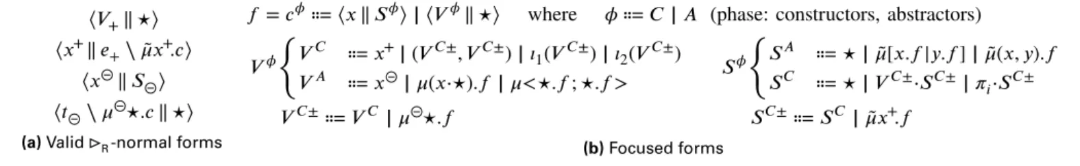
Figure 7a describes the syntax of valid ⊳R-normal forms,
where a constructor is never opposed to an abstractor for another connective. For example ⟨𝜄1(𝑡) ‖ ̃𝜇(𝑥, 𝑦).𝑐⟩ would be an invalid
normal form. A normal command of the form ⟨𝑉+‖ ⋆⟩ or
⟨𝑉+‖ ⋆⟩
⟨𝑥+‖ 𝑒+⧵ ̃𝜇𝑥+.𝑐⟩ ⟨𝑥⊝‖ 𝑆⊝⟩
⟨𝑡⊝⧵ 𝜇⊝⋆.𝑐 ‖ ⋆⟩
(a) Valid⊳R-normal forms
𝑓 = 𝑐𝜙⩴ ⟨𝑥 ‖ 𝑆𝜙⟩ | ⟨𝑉𝜙‖ ⋆⟩ where 𝜙 ⩴ 𝐶 | 𝐴 (phase: constructors, abstractors) 𝑉𝜙 { 𝑉𝐶 ⩴ 𝑥+| (𝑉𝐶±, 𝑉𝐶±) | 𝜄1(𝑉𝐶±) | 𝜄2(𝑉𝐶±) 𝑉𝐴 ⩴ 𝑥⊝| 𝜇(𝑥⋅⋆).𝑓 | 𝜇<⋆.𝑓 ; ⋆.𝑓 > 𝑉𝐶±⩴ 𝑉𝐶 | 𝜇⊝⋆.𝑓 𝑆𝜙 { 𝑆𝐴 ⩴ ⋆ | ̃𝜇[𝑥.𝑓|𝑦.𝑓 ] | ̃𝜇(𝑥, 𝑦).𝑓 𝑆𝐶 ⩴ ⋆ | 𝑉𝐶±⋅𝑆𝐶±| 𝜋𝑖⋅𝑆𝐶± 𝑆𝐶±⩴ 𝑆𝐶 | ̃𝜇𝑥+.𝑓 (b) Focused forms — Figure 7 – Normal and focused forms
A command of the form ⟨𝑥+‖ 𝑒+⧵ ̃𝜇𝑥+.𝑐 ⟩ (any 𝑒+ that is not a 𝜇𝑥̃ +.𝑐) or ⟨𝑡⊝⧵ 𝜇⊝⋆.𝑐 ‖ ⋆⟩ starts with an abstractor whose computation is blocked by the lack of information on the opposite side. We therefore decompose the structure of normal commands as a succession of phases, with constructor phases 𝑐𝐶 and abstractor phases 𝑐𝐴.
Figure 7b describes the structure of phase-separated →R -normal forms. We call them focused forms. A focused form 𝑓 is a focused command 𝑐𝜙 for some phase variable 𝜙, which is either 𝐶 or 𝐴—we will write ̄𝜙 for the phase opposite to 𝜙. A focused command 𝑐𝜙is either a focused value 𝑉𝜙against ⋆, or a focused stack 𝑆𝜙against some variable 𝑥. Constructor values 𝑉𝐶 start with a head expression constructor, followed by other head constructors until 𝜇⊝⋆.𝑓 or a variable is reached, ending the phase. Constructor stacks 𝑆𝐶 are non-empty compositions of stack constructors ended by a 𝜇𝑥̃ +.𝑓 . Abstractor values or stacks are either a variable or ⋆, or a 𝜇-form that immediately ends the phase.
This syntactic phase separation resembles focused proofs [4]. We work in an untyped calculus, so we cannot enforce that phases be maximally long; but otherwise constructor phases correspond to non-invertible, or synchronous rules, while ab-stractor phases correspond to invertible, or asynchronous infer-ence rules.
Not all →R-normal forms are focused forms in the sense
of Figure7b because they may not respect the constraint that phase change must be explicitly marked by a 𝜇 or 𝜇 (for̃ example with ⟨𝜄1(𝑥⊝) ‖ ⋆⟩). But a normal form can be easily
rewritten into a focused form by trivial (→E𝜇 ̃𝜇)-expansions
(⟨𝜄1(𝜇⊝⋆.⟨𝑥⊝‖ ⋆⟩) ‖ ⋆⟩ in our example).
Lemma 6. Any valid →R-normal form (→∗E
𝜇, ̃𝜇)-expands to a unique focused form 𝑓 .
B. Algorithmic equality for expansion rules
a) Restriction to SN terms: We study the equivalence of →R-normal forms modulo →R-strongly-normalising (SN) conversions. Therefore we set ourselves in the subset LSNint of SN terms of Lint. This is a more general alternative to studying
the equivalence modulo well-typed conversions for some type system. Notice that since →R is confluent, any SN term has a
unique →R-normal form.
LSNint is not closed under ≃RE, since any strongly-normalizable command is equivalent to some non-normalizable commands. We define ⊳SNR and ⊳SNE by restriction of ⊳R and ⊳E to LSNint. The SN-compatible closure →SN of ⊳SN is defined such that 𝑝 →SN𝑝′for 𝑝, 𝑝′two SN terms whenever 𝑝′is obtained from 𝑝 by application of ⊳SN on one of its sub-commands. Then ≃SN is defined as the equivalence closure of →SN.
b) Algorithmic equality: Now we show that ≃SNRE is de-cidable, by defining a form of algorithmic equality on normal forms, and we deduce that ≃SNRE is not inconsistent.
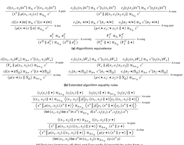
We define the algorithmic equality relation ≡A as a system
of inference rules on pairs of SN commands, which captures extensional equivalence: ≡A decides ≃SNE . If we had worked on typed normal forms, we could have performed some maximal, type-directed, →E-expansion. However, for the sake of
general-ity and its intrinsic interest, we work with Curry-style normal forms.
The purely syntactic approach performs, in both of the commands to be compared, the →E-expansions for the abstrac-tors that appear in either command. This untyped equivalence is inspired by previous works (Coquand [10]; Abel and Co-quand [1]) where the 𝜂-equivalence of 𝜆-terms is computed by looking at the terms only, by doing an 𝜂-expansion when either term starts with 𝜆.
In Figure 8a, we define ≡A on SN commands by mutual recursion with a sub-relation ≡A
𝑁, the latter of which only relates →R-normal forms.
We have omitted the symmetric counterparts for the abstrac-tor rules. In the last two cases, we consider that ≡A is defined on expressions and contexts as the congruence closure of ≡A on sub-commands. For example, 𝜄1(𝜇⋆.𝑐 ) ≡A 𝑡′ if and only if 𝑡′ is of the form 𝜄1(𝜇⋆.𝑐′) for some 𝑐′ such that 𝑐 ≡A 𝑐′.
We use the term algorithmic because this equivalence is almost syntax-directed. If both sides of the equivalence start with an abstractor application, there is a non-syntax-directed choice of which side to inspect first: for 𝑡, 𝑢 fixed there may be several distinct derivations of 𝑡 ≡A 𝑢.
Algorithmic equivalence is well-defined because since the commands in the conclusion of the form ≡A𝑁 are normal,
the commands in their premises are SN, hence they can be compared through ≡A. Indeed, whenever 𝑐 is a →R-normal
form, the substitutions applied by those rules (for instance 𝑐[ (𝑥1, 𝑥2)/𝑥+]) may create new redexes (for instance with
𝑐 = ⟨𝑥+‖ 𝜇(𝑦1, 𝑦2).𝑐′⟩ ), but contracting such redexes only
creates substitutions of variables for variables ([ 𝑥1/𝑦1] and
[𝑥2/𝑦2] in this example). In particular any reduction path has
a length of at most the number of occurrences of the variable (𝑥+in the example).
Lemma 7. Soundness of algorithmic equivalence: if 𝑡 ≡A 𝑢
then 𝑡 ≃SNRE 𝑢.
C. Completeness of algorithmic equality on normal forms Abel and Coquand [1] discuss the problem of transitivity of their syntax-directed algorithmic equality: while it morally captures our intuition of valid 𝜂-equivalences, it fails to account for some seemingly-absurd equivalences that can be derived on untyped terms, such as 𝜆𝑥.(𝑡 𝑥) ≃𝜂 <𝜋1𝑡; 𝜋2𝑡>, the transitive
𝑐 →∗R 𝑐1(↛) 𝑐1≡A𝑁 𝑐1′ (↚)𝑐1′←∗R 𝑐′ —A-R 𝑐 ≡A 𝑐′ 𝑐[(𝑥1, 𝑥2)/𝑥+] ≡A 𝑐′[(𝑥1, 𝑥2)/𝑥+] —A-pair ⟨𝑥+‖ 𝜇(𝑥1, 𝑥2).𝑐⟩ ≡A 𝑁 𝑐 ′ 𝑐1[𝜄1(𝑥1)/𝑥+] ≡A 𝑐′[𝜄1(𝑥1)/𝑥+] 𝑐2[𝜄2(𝑥2)/𝑥+] ≡A𝑐′[𝜄2(𝑥2)/𝑥+] —A-sum ⟨𝑥+‖ ̃𝜇[𝑥1.𝑐1|𝑥2.𝑐2]⟩ ≡A 𝑁 𝑐 ′ 𝑐[(𝑥⋅⋆)/𝛼] ≡A𝑐′[(𝑥⋅⋆)/⋆] —A-fun ⟨𝜇(𝑥⋅⋆).𝑐 ‖ 𝛼⟩ ≡A𝑁 𝑐′ 𝑐1[𝜋1⋅⋆/⋆] ≡A 𝑐′[𝜋1⋅⋆/⋆] 𝑐2[𝜋2⋅⋆/⋆] ≡A𝑐′[𝜋2⋅⋆/⋆] —A-neg-pair ⟨𝜇<⋆.𝑐1; ⋆.𝑐2> ‖ ⋆⟩ ≡A𝑁 𝑐′ 𝜋1𝐶 ≡A 𝜋2𝐶 —A-cocong ⟨𝑥⊝‖ 𝜋1𝐶⟩ ≡A 𝑁 ⟨𝑥 ⊝‖ 𝜋𝐶 2⟩ 𝑉1𝐶 ≡A 𝑉2𝐶 —A-cong ⟨𝑉1𝐶‖ ⋆⟩ ≡A 𝑁 ⟨𝑉 𝐶 2 ‖ ⋆⟩
(a) Algorithmic equivalence 𝑐[(𝑥1, 𝑥2)/𝑉+] ≡A+ 𝑐′[(𝑥1, 𝑥2)/𝑉+] —A+pair ⟨𝑉+‖ 𝜇(𝑥1, 𝑥2).𝑐⟩ ≡A+ 𝑁 𝑐 ′ 𝑐1[𝜄1(𝑥1)/𝑉+] ≡A𝑐′[𝜄1(𝑥1)/𝑉+] 𝑐2[𝜄2(𝑥1)/𝑉+] ≡A 𝑐′[𝜄2(𝑥1)/𝑉+] —A+sum ⟨𝑉+‖ ̃𝜇[𝑥1.𝑐1|𝑥2.𝑐2]⟩ ≡A+ 𝑁 𝑐 ′ 𝑐[(𝑥⋅⋆)/𝑆⊝] ≡A+𝑐′[(𝑥⋅⋆)/𝑆⊝] —A+fun ⟨𝜇(𝑥⋅⋆).𝑐 ‖ 𝑆⊝⟩ ≡A+ 𝑁 𝑐 ′ 𝑐1[𝜋1⋅⋆/𝑆⊝] ≡A+𝑐′[𝜋1⋅⋆/𝑆⊝] 𝑐1[𝜋2⋅⋆/𝑆⊝] ≡A+𝑐′[𝜋2⋅⋆/𝑆⊝] —A+negpair ⟨𝜇<⋆.𝑐1; ⋆.𝑐2> ‖ 𝑆⊝⟩ ≡A+ 𝑁 𝑐 ′
(b) Extended algorithm equality rules ⟨𝜄1(𝑦1) ‖ ⋆⟩ ≡A+ 𝑁 ⟨𝜄1(𝑦1) ‖ ⋆⟩ ⟨𝜄2(𝑦1) ‖ ⋆⟩ ≡A+𝑁 ⟨𝜄2(𝑦1) ‖ ⋆⟩ —A+sum ⟨(𝑥1, 𝑥2) ‖ ⋆⟩ ≡A+𝑁 ⟨(𝑥1, 𝑥2) ‖ ̃𝜇[𝑦1.⟨(𝑥1, 𝑥2) ‖ ⋆⟩|𝑦2.⟨(𝑥1, 𝑥2) ‖ ⋆⟩]⟩ —A+pair ⟨𝑥+‖ 𝜇(𝑥1, 𝑥2).⟨𝑥+‖ ⋆⟩⟩ ≡A+𝑁 ⟨𝑥+‖ ̃𝜇[𝑦1.⟨𝑥+‖ ⋆⟩|𝑦2.⟨𝑥+‖ ⋆⟩]⟩ — (let(𝑥1, 𝑥2)be𝑥+in𝑥+) ≡A+ 𝑁 𝛿(𝑥 +, 𝜄 1(𝑦1).𝑥+, 𝜄2(𝑦2).𝑥+) ⟨(𝑥1, 𝑥2) ‖ 𝑦⋅⋆⟩ ≡A+𝑁 ⟨(𝑥1, 𝑥2) ‖ 𝑦⋅⋆⟩ —A+pair ⟨𝑥+‖ 𝜇(𝑥1, 𝑥2).⟨(𝑥1, 𝑥2) ‖ 𝑦⋅⋆⟩⟩ ≡A+𝑁 ⟨𝑥+‖ 𝑦⋅⋆⟩ —A+fun ⟨𝑥+‖ 𝜇(𝑥1, 𝑥2).⟨(𝑥1, 𝑥2) ‖ ⋆⟩⟩ ≡A+𝑁 ⟨𝜇(𝑦⋅⋆).⟨𝑥+‖ 𝑦⋅⋆⟩ ‖ ⋆⟩ — (let(𝑥1, 𝑥2)be𝑥+in(𝑥1, 𝑥2)) ≡A+𝑁 𝜆𝑦.(𝑥+𝑦)
(c) Deriving (instances of) Abel and Coquand’s [1] transitivity rules from≡A+.
— Figure 8 – Algorithmic equivalence
combination of 𝜆𝑥.(𝑡 𝑥) ≃𝜂 𝑡 and 𝑡 ≃𝜂 <𝜋1𝑡; 𝜋2𝑡>. To account for those absurd equivalences, Abel and Coquand had to extend their relation with type-incorrect rules such as:
𝑡 ≡A𝑛 𝑥 𝜋1𝑛 ≡A𝑟 𝜋2𝑟 ≡A 𝑠
— 𝜆𝑥.(𝑡 𝑥) ≡A <𝑟; 𝑠>
This change suffices to regain transitivity and capture untyped 𝜂-conversion. Unfortunately, this technique requires a number of additional rules quadratic in the number of different construc-tors of the language. Our richer syntax allows the definition in Figure8bof an extended algorithmic equivalence ≡A+without
introducing any new rule. Instead, we extend each constructor rule A-fun, A-pair, etc., in a simple (but potentially type-incorrect) way.
We introduce the notation 𝑐[𝑡/𝑉 ] which substitutes syntactic occurrences of the term 𝑉 by 𝑡—there is a unique decomposi-tion of 𝑐 into 𝑐′[𝑉 /𝑥] with 𝑉 ∉ 𝑐′, and then 𝑐[𝑡/𝑉 ] is defined as 𝑐′[𝑡/𝑥]. On valid terms, this extended equivalence coincides with the previous algorithmic equivalence. Indeed, in the case of a normal command ⟨𝑉+‖ 𝜇(𝑥1, 𝑥2).𝑐⟩ for example, a valid
𝑉+ can only be a variable 𝑥+, in which case the rule A-pair
and A+pair are identical. The extension only applies when 𝑉+
has a head constructor that is not the pair, in which case the expression is in normal form but invalid.
Figure 8c shows that this extension subsumes the rules of Abel and Coquand. Notice how the inference following the leftmost leaf is obtained by the apparently-nonsensical substitution ⟨ (𝑥1, 𝑥2) ‖ ⋆ ⟩ [ 𝜄1𝑦1/(𝑥1, 𝑥2) ] produced by the
extended sum rule on an invalid command. Lemma 8 (Soundness). One has ≡A+⊆ ≃SNRE. Lemma 9 (Reflexivity). If 𝑡 is SN then 𝑡 ≡A+𝑡.
Lemma 10 (Transitivity). If 𝑡1 ≡A+ 𝑡2 and 𝑡2 ≡A+ 𝑡3 then
𝑡1≡A+𝑡3.
Lemma 11 (Completeness). If 𝑐 ≃SNRE 𝑐′then 𝑐 ≡A+𝑐′.
Theorem 12. 𝑐1≃SNRE 𝑐2if and only if 𝑐1≡A+𝑐2. Corollary 13. ≃SNRE is consistent.
Indeed, ⟨ 𝑥+ ‖ ⋆ ⟩ is not algorithmically equivalent to ⟨𝑦+‖ ⋆⟩. This result on ≃SNRE does not allow us to prove our conjecture that ≃RE is consistent: notice that in the case of the
untyped 𝜆-calculus with sums, the inconsistency indeed relies on non-normalizing intermediate conversion steps, involving the fixed point of 𝜆𝑥.𝛿(𝑥, 𝑦.𝜄2(𝑦), 𝑦.𝜄1(𝑦)) as we recalled in the