Conflict-Free Coloring of Graphs
The MIT Faculty has made this article openly available.
Please share
how this access benefits you. Your story matters.
Citation
Abel, Zachary et al. "Conflict-Free Coloring of Graphs." SIAM
Journal on Discrete Mathematics 32, 4 (2018): 2675–2702 © 2018
The Author(s)
As Published
http://dx.doi.org/10.1137/17m1146579
Publisher
Society for Industrial & Applied Mathematics
Version
Final published version
Citable link
https://hdl.handle.net/1721.1/122951
Terms of Use
Article is made available in accordance with the publisher's
policy and may be subject to US copyright law. Please refer to the
publisher's site for terms of use.
CONFLICT-FREE COLORING OF GRAPHS\ast
ZACHARY ABEL\dagger , VICTOR ALVAREZ\ddagger , ERIK D. DEMAINE\S , S \'ANDOR P. FEKETE\ddagger ,
AMAN GOUR\P , ADAM HESTERBERG\dagger , PHILLIP KELDENICH\ddagger , AND
CHRISTIAN SCHEFFER\ddagger
Abstract. A conflict-free k-coloring of a graph assigns one of k different colors to some of the vertices such that, for every vertex v, there is a color that is assigned to exactly one vertex among v and v's neighbors. Such colorings have applications in wireless networking, robotics, and geometry and are well studied in graph theory. Here we study the natural problem of the conflict-free chromatic number \chi CF(G) (the smallest k for which conflict-free k-colorings exist). We provide
results both for closed neighborhoods N [v], for which a vertex v is a member of its neighborhood, and for open neighborhoods N (v), for which vertex v is not a member of its neighborhood. For closed neighborhoods, we prove the conflict-free variant of the famous Hadwiger Conjecture: If an arbitrary graph G does not contain Kk+1as a minor, then \chi CF(G) \leq k. For planar graphs, we obtain a tight
worst-case bound: three colors are sometimes necessary and always sufficient. In addition, we give a complete characterization of the algorithmic/computational complexity of conflict-free coloring. It is NP-complete to decide whether a planar graph has a conflict-free coloring with one color, while for outerplanar graphs, this can be decided in polynomial time. Furthermore, it is NP-complete to decide whether a planar graph has a conflict-free coloring with two colors, while for outerplanar graphs, two colors always suffice. For the bicriteria problem of minimizing the number of colored vertices subject to a given bound k on the number of colors, we give a full algorithmic characterization in terms of complexity and approximation for outerplanar and planar graphs. For open neighborhoods, we show that every planar bipartite graph has a conflict-free coloring with at most four colors; on the other hand, we prove that for k \in \{ 1, 2, 3\} , it is NP-complete to decide whether a planar bipartite graph has a conflict-free k-coloring. Moreover, we establish that any general planar graph has a conflict-free coloring with at most eight colors.
Key words. conflict-free coloring, planar graphs, complexity, worst-case bounds AMS subject classifications. 05C10, 05C15, 05C69, 05C83
DOI. 10.1137/17M1146579
1. Introduction. Coloring the vertices of a graph is one of the fundamental
problems in graph theory, both scientifically and historically. Proving that four colors always suffice to color a planar graph [6, 7, 27] was a tantalizing open problem for more than 100 years; the quest for solving this challenge contributed to the development of graph theory, but also to computers in theorem proving [29]. A generalization that is still unsolved is the Hadwiger Conjecture [19]: A graph is k-colorable if it has no
Kk+1minor.
\ast Received by the editors September 7, 2017; accepted for publication (in revised form) September 10,
2018; published electronically November 27, 2018. An extended abstract containing major parts of this paper was entitled Three colors suffice: Conflict-free coloring of planar graphs and appeared in the Proceedings of the Twenty-Eighth Annual ACM-SIAM Symposium on Discrete Algorithms (SODA 2017) [2].
http://www.siam.org/journals/sidma/32-4/M114657.html
Funding: Work on this paper was partially supported by the DFG Research Unit Controlling Concurrent Change, funding number FOR 1800, project FE407/17-2, Conflict Resolution and Optimization.
\dagger Mathematics Department, MIT, Cambridge, MA 02139 ([email protected], achesterberg@gmail.
com).
\ddagger Department of Computer Science, Braunschweig University of Technology, 38106 Braunschweig,
Germany ([email protected], [email protected], [email protected], [email protected]).
\S CSAIL, MIT, Cambridge, MA 02139 ([email protected]).
\P Department of Computer Science and Engineering, IIT Bombay, Mumbai, India (amangour30@
gmail.com).
2675
Over the years, there have been many variations on coloring, often motivated by particular applications. One such context is wireless communication, where ``colors"" correspond to different frequencies. This also plays a role in robot navigation, where different beacons are used for providing direction. To this end, it is vital that in any given location, a robot is adjacent to a beacon with a frequency that is unique among the ones that can be received. This notion has been introduced as conflict-free coloring,
formalized as follows. For any vertex v\in V of a simple graph G = (V, E), the closed
neighborhood N [v] consists of all vertices adjacent to v and v itself. A conflict-free
k-coloring of G assigns one of k different colors to a (possibly proper) subset S\subseteq V
of vertices, such that for every vertex v \in V , there is a vertex y \in N[v], called the
conflict-free neighbor of v, such that the color of y is unique in the closed neighborhood
of v. The conflict-free chromatic number \chi CF(G) of G is the smallest k for which
a conflict-free coloring exists. Observe that \chi CF(G) is bounded from above by the
proper chromatic number \chi (G) because in a proper coloring, every vertex is its own conflict-free neighbor. Similar questions can be considered for open neighborhoods N (v) = N [v]\setminus \{ v\} .
Conflict-free coloring has received an increasing amount of attention. Because of the relationship to classic coloring, it is natural to investigate the conflict-free coloring of planar graphs. In addition, previous work has considered either general graphs and hypergraphs (e.g., see [26]) or geometric scenarios (e.g., see [21]); we give a more detailed overview in what follows. This adds to the relevance of conflict-free coloring of planar graphs, which constitute the intersection of general graphs and geometry. In addition, the subclass of outerplanar graphs is of interest, as it corresponds to subdividing simple polygons by chords.
There is a spectrum of different scientific challenges when studying conflict-free coloring. What are worst-case bounds on the necessary number of colors? When is it NP-hard to determine the existence of a conflict-free k-coloring? When is it polynomially solvable? What can be said about approximation? Are there sufficient conditions for more general graphs? And what can be said about the bicriteria problem, in which also the number of colored vertices is considered? We provide extensive answers for all of these aspects, basically providing a complete characterization for planar and outerplanar graphs.
1.1. Our contribution. We present the following results; items 1--7 are for
closed neighborhoods, while items 8--10 are for open neighborhoods.
1. For general graphs, we provide the conflict-free variant of the Hadwiger
Conjecture: If G does not contain Kk+1 as a minor, then \chi CF(G)\leq k.
2. It is NP-complete to decide whether a planar graph has a conflict-free coloring with one color. For outerplanar graphs, this question can be decided in polynomial time.
3. It is NP-complete to decide whether a planar graph has a conflict-free coloring with two colors. For outerplanar graphs, two colors always suffice.
4. Three colors are sometimes necessary and always sufficient for conflict-free coloring of a planar graph.
5. For the bicriteria problem of minimizing the number of colored vertices subject
to a given bound \chi CF(G)\leq k with k \in \{ 1, 2\} , we prove that the problem is
NP-hard for planar and polynomially solvable in outerplanar graphs. 6. For planar graphs and k = 3 colors, minimizing the number of colored vertices
does not have a constant-factor approximation unless P = NP.
7. For planar graphs and k\geq 4 colors, it is NP-complete to minimize the number of colored vertices. The problem is fixed-parameter tractable (FPT) and allows a polynomial-time approximation scheme (PTAS).
8. Four colors are sometimes necessary and always sufficient for conflict-free coloring with open neighborhoods of planar bipartite graphs.
9. It is NP-complete to decide whether a planar bipartite graph has a conflict-free
coloring with open neighborhoods with k colors for k\in \{ 1, 2, 3\} .
10. Eight colors always suffice for conflict-free coloring with open neighborhoods of planar graphs.
1.2. Related work. In a geometric context, the study of conflict-free coloring
was started by Even et al. [16] and Smorodinsky [28], who motivate the problem by frequency assignment in cellular networks: There, a set of n base stations is given, each covering some geometric region in the plane. The base stations service mobile clients that can be at any point in the total covered area. To avoid interference, there must be at least one base station in range using a unique frequency for every point in the entire covered area. The task is to assign a frequency to each base station minimizing the number of frequencies. On an abstract level, this induces a coloring problem on a hypergraph where the base stations correspond to the vertices and there is a hyperedge between some vertices if the range of the corresponding base stations has a nonempty common intersection.
If the hypergraph is induced by disks, Even et al. [16] prove that\scrO (log n) colors are
always sufficient. Alon and Smorodinsky [5] extend this by showing that each family of
disks, where each disk intersects at most k others, can be colored using\scrO (log3k) colors.
Furthermore, for unit disks, Lev-Tov and Peleg [24] present an\scrO (1)-approximation
algorithm for the number of colors. Horev, Krakovski, and Smorodinsky [22] extend
this by showing that any set of n disks can be colored with\scrO (k log n) colors, even if
every point must see k distinct unique colors. Abam, de Berg, and Poon [1] discuss the problem in the context of cellular networks where the network has to be reliable even if some number of base stations fail, giving worst-case bounds for the number of colors required.
For the dual problem of coloring a set of points such that each region from some family of regions contains at least one uniquely colored point, Har-Peled and Smorodinsky [20] prove that with respect to every family of pseudo-disks, every set
of points can be colored using\scrO (log n) colors. For rectangle ranges, Elbassioni and
Mustafa [15] show that it is possible to add a sublinear number of points such that
a conflict-free coloring with\scrO (n3/8\cdot (1+\varepsilon )) colors becomes possible. Ajwani et al. [3]
complement this by showing that coloring a set of points with respect to rectangle
ranges is always possible using \scrO (n0.382) colors. For coloring points on a line with
respect to intervals, Cheilaris et al. [11] present a 2-approximation algorithm, and a\bigl( 5 - 2
k\bigr) -approximation algorithm when every interval must see k uniquely colored
vertices. Hoffman et al. [21] give tight bounds for the conflict-free chromatic art gallery problem under rectangular visibility in orthogonal polygons: \Theta (log log n) are sometimes necessary and always sufficient. Chen et al. [14] consider the online version of the conflict-free coloring of a set of points on the line, where each newly inserted point must be assigned a color upon insertion, and at all times the coloring has to be conflict-free. Also in the online scenario, Bar-Noy et al. [10] consider a certain class of k-degenerate hypergraphs which sometimes arise as intersection graphs of geometric
objects, presenting an online algorithm using\scrO (k log n) colors.
On the combinatorial side, some authors consider the variant in which all vertices need to be colored; note that this does not change asymptotic results for general graphs and hypergraphs: it suffices to introduce one additional color for vertices that are left uncolored in our constructions. Regarding general hypergraphs, Ashok, Dudeja, and Kolay [8] prove that maximizing the number of conflict-freely colored edges in a hypergraph is FPT when parameterized by the number of conflict-free edges in the solution. Cheilaris, Smorodinsky, and Sulovsky [12] consider the case of hypergraphs induced by a set of planar Jordan regions and prove an asymptotically tight upper
bound of \scrO (log n) for the conflict-free list chromatic number of such hypergraphs.
They also consider hypergraphs induced by the simple paths of a planar graph and
prove an upper bound of \scrO (\surd n) for the conflict-free list chromatic number. For
hypergraphs induced by the paths of a simple graph G, Cheilaris and T\'oth [13] prove
that it is coNP-complete to decide whether a given coloring is conflict-free if the input is G. Regarding the case in which the hypergraph is induced by the neighborhoods of
a simple graph G, which resembles our scenario, Pach and T\'ardos [26] prove that the
conflict-free chromatic number of an n-vertex graph is in\scrO (log2n). Glebov, Szab\'o, and
Tardos [18] extend this from an extremal and probabilistic point of view by proving that
almost all G(n, p)-graphs have conflict-free chromatic number\scrO (log n) for p \in \omega (1/n),
and by giving a randomized construction for graphs having conflict-free chromatic
number \Theta (log2n). In more recent work, Gargano and Rescigno [17] show that finding
the conflict-free chromatic number for general graphs is NP-complete, and prove that the problem is FPT with respect to vertex cover or neighborhood diversity number.
2. Preliminaries. For every vertex v \in V , the open neighborhood of v in G is
denoted by NG(v) :=\{ w \in V (G) | vw \in E(G)\} , and the closed neighborhood is denoted
by NG[v] := NG(v)\cup \{ v\} . We sometimes write N(v) instead of NG(v) when G is clear
from the context.
A partial k-coloring of G is an assignment \chi : V\prime
\rightarrow \{ 1, . . . , k\} of colors to a subset V\prime
\subseteq V (G) of the vertices. \chi is called closed-neighborhood conflict-free k-coloring of G
iff, for each vertex v\in V , there is a vertex w \in NG[v]\cap V\prime such that \chi (w) is unique
in NG[v], i.e., for all other w\prime \in NG[v]\cap V\prime , \chi (w\prime )\not = \chi (w). We call w the conflict-free neighbor of v. Analogously, \chi is called open-neighborhood conflict-free k-coloring of G
iff, for each vertex v\in V , there is a conflict-free neighbor w \in NG(v).
In order to avoid confusion with proper k-colorings, i.e., colorings that color all vertices such that no adjacent vertices receive the same color, we use the term proper
coloring when referring to this kind of coloring. The minimum number of colors needed
for a proper coloring of G, also known as the chromatic number of G, is denoted by
\chi P(G), whereas the minimum number of colors required for a closed-neighborhood
conflict-free coloring of G (G's closed-neighborhood conflict-free chromatic number )
is written as \chi CF(G). The open-neighborhood conflict-free chromatic number of G is
\chi O(G). To improve readability we sometimes omit the type of neighborhood if it is
clear from the context.
Note that, because every vertex satisfies v \in N[v], every proper coloring of G
is also a closed-neighborhood conflict-free coloring of G, and thus \chi CF(G)\leq \chi P(G).
The same does not hold for open neighborhoods. There is no constant factor c1> 0
such that either c1\cdot \chi O(G)\leq \chi P(G) or c1\cdot \chi P(G)\leq \chi O(G) holds for all graphs G.
For closed neighborhoods, we define the conflict-free domination number \gamma k
CF(G)
of G to be the minimum number of vertices that have to be colored in a conflict-free
k-coloring of G. We set \gamma k
CF(G) = \infty if G is not conflict-free k-colorable. Because
the set of colored vertices is a dominating set, the conflict-free domination number
satisfies \gamma k
CF(G)\geq \gamma (G) for all k, where \gamma (G), the domination number of G, is the
size of a minimum dominating set of G. Moreover, for any graph, there is a k\leq \gamma (G)
such that \gamma k
CF(G) = \gamma (G).
We denote the complete graph on n vertices by Kn:= (\{ 1, . . . , n\} , \{ \{ u, v\} | u, v \in
\{ 1, . . . , n\} , u \not = v\} ), and the complete bipartite graph on n and m vertices as Kn,m.
We define the graph K - 3
n := (V (Kn), E(Kn)\setminus E(K3)), which is obtained by removing
any three edges forming a single triangle from a Kn.
We also provide a number of results for outerplanar graphs. An outerplanar graph is a graph that has a planar embedding for which all vertices belong to the outer face of the embedding. An outerplanar graph is called maximal iff no edges can be added to the graph without losing outerplanarity [9]. Maximal outerplanar graphs can also be characterized as the graphs having an embedding corresponding to a polygon triangulation, which illustrates their particular relevance in a geometric context. In addition, maximal outerplanar graphs exhibit a number of interesting graph-theoretic properties. Every maximal outerplanar graph is chordal, a 2-tree, and a series-parallel graph. Also, every maximal outerplanar graph is the visibility graph of a simple polygon.
For some of our NP-hardness proofs, we use a variant of the planar 3-SAT problem, called Positive Planar 1-in-3-SAT. This problem was introduced and shown to be NP-complete by Mulzer and Rote [25] and consists of deciding whether a given positive planar formula in conjunctive normal form with at most 3 literals per clause (3-CNF) allows a truth assignment such that in each clause, exactly one literal is true.
Definition 2.1 (positive planar formulas). A formula \phi in 3-CNF is called
positive planar iff it is both positive and backbone planar. A formula \phi is called positive iff it does not contain any negation, i.e., iff all occurring literals are positive.
A formula \phi , with clause set C =\{ c1, . . . , cl\} and variable set X = \{ x1, . . . , xn\} , is
called backbone planar iff its associated graph G(\phi ) := (X\cup C, E(\phi )) is planar, where
E(\phi ) is defined as follows:
\bullet xicj\in E(\phi ) for a clause cj \in C and a variable xi \in X iff xi occurs incj,
\bullet xixi+1\in E(\phi ) for all 1 \leq i < n.
The path formed by the latter edges is also called the backbone of the formula graph
G(\phi ).
3. Closed neighborhoods: Conflict-free coloring of general graphs. In
this section we consider the Conflict-Free k-Coloring problem on general simple graphs with respect to closed neighborhoods. In section 3.1, we prove that this
problem is NP-complete for any k\geq 1. In section 3.2, we provide a sufficient criterion
that guarantees free k-colorability. In section 3.3, we consider the
conflict-free domination number and prove that, for any k \geq 3, there is no constant-factor
approximation algorithm for \gamma k
CF.
3.1. Complexity.
Theorem 3.1. Conflict-Free k-Coloring is NP-complete for any fixed k\geq 1.
Membership in NP is clear. For k\geq 3, we prove NP-hardness using a reduction
from Proper k-Coloring. For k \in \{ 1, 2\} , refer to section 4, where we prove
Conflict-Free k-Coloring of planar graphs to be NP-complete for k\in \{ 1, 2\} .
Central to the proof is the following lemma, which enables us to enforce certain vertices to be colored, and both ends of an edge to be colored using distinct colors.
Lemma 3.2. Let G be any graph, u, v \in V (G), and vu = e \in E(G). If N(v)
contains two disjoint and independent copies of a graph H with \chi CF(H) = k, not
adjacent to any other vertex w\in G, every conflict-free k-coloring of G colors v. If
the same holds for u and, in addition, NG(u)\cap NG(v) contains two disjoint and
independent copies of a graphJ with \chi CF(J) = k - 1, not adjacent to any other vertex
w\in G, every conflict-free k-coloring of G colors u and v with different colors.
Proof. Assume towards a contradiction that there was a conflict-free k-coloring \chi
that avoids coloring v. Then, due to the copies of H being independent, disjoint, and not connected to any other vertex, the restriction of \chi to the vertices of each of the
two copies must induce a conflict-free coloring on H. As \chi CF(H) = k, this implies
that \chi uses k colors on each copy. Therefore, in the open neighborhood of v, there are at least two vertices colored with each color. This leads to a contradiction, because v cannot have a conflict-free neighbor.
For the second proposition, suppose there was a conflict-free coloring assigning the same color to u and v. Without loss of generality, let this color be 1. As every vertex of the two copies of J now sees two occurrences of color 1, color 1 cannot be the color of the unique neighbor of any vertex of J, and any occurrence of color 1 on the vertices of J can be removed. Therefore, we can assume each of the two copies of J to
be colored in a conflict-free manner using the colors\{ 2, . . . , k\} . Observe that, due to
\chi CF(J) = k - 1, each of these colors must be used at least once in each copy. This
implies that both u and v see each color at least twice: The two copies of J enforce
two occurrences of the colors\{ 2, . . . , k\} , and color 1 is assigned to both u and v, which
are connected by an edge. This is a contradiction, and therefore, both u and v must be colored with distinct colors.
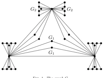
Next, we give an inductive construction of graphs, Gk, with \chi CF(Gk) = k. The
proof of NP-hardness relies on this hierarchy.
1. The first graph G1 of the hierarchy consists of a single isolated vertex. G2is
a K1,3 with one edge subdivided by another vertex, or, equivalently, a path of
length 3 with a leaf vertex attached to one of the inner vertices.
2. Given Gk and Gk - 1, Gk+1is constructed as follows for k\geq 2:
\bullet Take a complete graph G = Kk+1 on k + 1 vertices.
\bullet To each vertex v \in V (Kk+1), attach two disjoint and independent copies
of Gk, adding an edge from v to every vertex of both copies of Gk.
\bullet For each edge e = vw \in E(Kk+1), add two disjoint and independent
copies of Gk - 1, adding an edge from v and w to every vertex of both
copies.
The number of vertices of the graphs Gk obtained by the above construction satisfies
the recursive formula
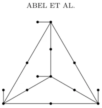
| G1| = 1, | G2| = 5, | Gk+1| = (k + 1) \cdot (2| Gk| + k| Gk - 1| + 1), which is in \Omega \bigl( 2k\bigr) and \scrO \bigl( 2k log k\bigr) . Figure 1 depicts the graph G
3, which in addition
to being planar is a series-parallel graph.
Lemma 3.3. For Gk constructed in this manner,\chi CF(Gk) = k.
Proof. The proof uses induction over k. Application of Lemma 3.2 implies that
all vertices of the Kk+1 underlying Gk+1 have to be colored using different colors.
Therefore, \chi CF(Gk+1)\geq k + 1. By coloring all k + 1 vertices of the underlying Kk+1
with a different color, we obtain a conflict-free (k + 1)-coloring of Gk+1, implying
\chi CF(Gk+1)\leq k + 1.
G2 G2
G1
G1
Fig. 1. The graph G3.
Lemma 3.4. For k\geq 2, k-Coloring \preccurlyeq Conflict-Free k-Coloring.
There-fore, fork\geq 3, Conflict-Free k-Coloring is NP-complete.
Proof. Given a graph G for which to decide proper k-colorability for a fixed k,
we construct a graph G\prime that is conflict-free k-colorable iff G is k-colorable. G\prime is
constructed from G by attaching two copies of Gk to each vertex v\in V (G), by adding
an edge from v to each vertex of the copies of Gk. For each edge uv\in E(G), we attach
two copies of Gk - 1 to both endpoints of uv by adding an edge from u and v to all
vertices of both copies. As k is fixed,| Gk| and | Gk - 1| are constant, implying that G\prime
can be constructed in polynomial time.
A proper k-coloring of G induces a conflict-free k-coloring of G\prime by leaving all
other vertices uncolored. On the other hand, by Lemma 3.2, a conflict-free k-coloring \chi of G\prime colors all vertices v
\in V (G) and for every edge, the colors of both endpoints are distinct. Therefore, the restriction of \chi to V (G) is a proper k-coloring of G.
3.2. A sufficient criterion for \bfitk -colorability. In this section we present a
sufficient criterion for conflict-free k-colorability together with an efficient heuristic that can be used to color graphs satisfying this criterion with k colors in a conflict-free manner. This heuristic is called iterated elimination of distance-3-sets and is detailed in Algorithm 3.1. The main idea of this heuristic is to iteratively compute maximal sets of vertices at pairwise (edge) distance at least 3, coloring all vertices in one of these sets using one color, and then removing these vertices and their neighbors until all that remains is a collection of disconnected paths, which can then be colored using one color.
Theorem 3.5. Let G be a graph and k \geq 1. If G has neither Kk+2 nor Kk+3 - 3
as a minor,G admits a conflict-free k-coloring that can be found in polynomial time
using iterated elimination of distance-3-sets.
Proof. For k = 1, a graph G with neither a K3 nor a K4 - 3= K1,3 minor consists
of a collection of isolated paths. A path on 3n vertices can be colored with one color by coloring the middle vertex of every three vertices. This does not color the vertices at either end, so up to two vertices can be removed from the path to get colorings for
paths on 3n - 1 and 3n - 2 vertices.
For k\geq 2, we use induction as follows: First, we color an inclusionwise maximal
subset D\subseteq V of vertices at pairwise distance at least 3 to each other using color 1.
Algorithm 3.1. Iterated elimination of distance-3-sets.
1: i\leftarrow 1, \chi \leftarrow \emptyset
2: Remove all isolated paths from G
3: while G is not empty do
4: D\leftarrow \emptyset
5: For each component of G, select some vertex v and add it to D
6: whilethere is a vertex w at distance\geq 3 from all vertices in D do
7: Choose w at distance exactly 3 from some vertex in D
8: D\leftarrow D \cup \{ w\}
9: \forall u \in D : \chi (u) \leftarrow i 10: i\leftarrow i + 1
11: Remove N [D] from G
12: Remove all isolated paths from G
13: Color all removed isolated paths using color i
This set D is chosen such that each vertex v \in D is at distance exactly 3 from some
v\prime \in D. Coloring D provides a conflict-free neighbor of color 1 to every vertex in N[D].
Therefore, the vertices in N [D] are covered and can be removed from the graph. The remaining graph consists of vertices at distance 2 to some vertex in D; we call these vertices unseen in the remainder of the proof. We show that the remaining graph has
no Kk+1and no Kk+2 - 3 as a minor. By induction, iterated elimination of distance-3-sets
requires k - 1 colors to color the remaining graph, and thus k colors suffice for G.
If the graph is disconnected, iterated elimination of distance-3-sets works on all components separately, so we can assume G to be connected. We claim that there is no set U of unseen vertices that is a cutset of G. Suppose there were such a cutset
U , and let H be any component of G\setminus U not containing v, the first selected vertex
during the construction of D. At least one vertex of H is colored: every vertex in U is at distance at least two from every colored vertex not in H; therefore, every vertex in H is at distance at least 3 from every colored vertex not in H. Consider the iteration where the first vertex w of H is added to the set of colored vertices D. At this point, w is at distance exactly 3 from some colored vertex not in H. However, this implies w is adjacent to some vertex from U , contradicting the fact that all vertices in U are unseen.
Now, suppose for the sake of contradiction that the set W of unseen vertices
contains a Kk+1or Kk+2 - 3 minor. W is not the whole graph, because at least one vertex
is colored, so there must be a vertex v not in the Kk+1 or Kk+2 - 3 minor. For every
vertex w\in W , there is a path from v to w that intersects W only at w. Otherwise,
W\setminus \{ w\} would be a cutset separating v from w. So, if the graph induced by W had
a Kk+1 or Kk+2 - 3 minor, we could contract G\setminus W to a single vertex, which would be
adjacent to all vertices in W , yielding a Kk+2 or Kk+3 - 3 minor of G, which does not
exist.
Observe that Gk+1contains a Kk+3 - 3 as a minor, but not a Kk+2, proving that just
excluding Kk+2as a minor does not suffice to guarantee k-colorability. Moreover, note
that Kk+1 is a minor of Kk+2and Kk+3 - 3 .
This yields the following corollary, which is the conflict-free variant of the Hadwiger Conjecture.
Corollary 3.6. All graphs that do not have Kk+1 as a minor are conflict-free k-colorable.
3.3. Conflict-free domination number. In this section we consider the
prob-lem of minimizing the number of colored vertices in a conflict-free k-coloring for a fixed
k, which is equivalent to computing \gamma k
CF. We call the corresponding decision problem
k-Conflict-Free Dominating Set. We show that approximating the conflict-free domination number in general graphs is hard for any fixed k. In section 5 we discuss the k-Conflict-Free Dominating Set problem for planar graphs.
Theorem 3.7. Unless P = NP, for any k \geq 3, there is no polynomial-time
approximation algorithm for\gamma k
CF(G) with constant approximation factor.
Proof. We use a reduction from proper k-Coloring for the proof. Assume
towards a contradiction that there was a polynomial-time approximation algorithm for \gamma k
CF(G) with approximation factor c\geq 1. Let G be a graph on n vertices for which we
want to decide k-colorability. For each vertex v of G, add M := (n + 1)(c + 1) vertices
uv to G and connect them to v. For each edge vw of G, add M vertices uvw to G
and connect them to both v and w. Let G\prime be the resulting graph. Clearly, the size
of G\prime is polynomial in the size of G. Additionally, G\prime is planar if G is, and G\prime has a
conflict-free k-coloring of size n iff G is properly k-colorable: Any proper k-coloring of
G is a conflict-free k-coloring of G\prime , as every vertex added to G is either adjacent to
two distinctly colored vertices of G, or adjacent to just one vertex of G. Conversely,
let \chi be a conflict-free coloring of G\prime , coloring just n vertices. If \chi did not assign a
color to some vertex v of G, it would have to color all M \geq n + 1 neighbors of v. If \chi
assigned the same color to any pair v, w of vertices adjacent in G, it would have to color all M vertices adjacent only to v and w. Therefore, \chi is a proper coloring of G.
Running a c-approximation algorithm\scrA for \gamma k
CF on G\prime results in an approximate value
\scrA (G\prime )
\leq c \cdot \gamma k
CF(G\prime ). We have\scrA (G\prime )\leq c \cdot n < M if G is k-colorable, and \scrA (G\prime )\geq M if G is not; thus we could decide proper k-colorability in polynomial time.
4. Closed neighborhoods: Planar conflict-free coloring. This section deals
with the Planar Conflict-Free k-Coloring problem, which consists of deciding conflict-free k-colorability for fixed k on planar graphs. Due to the 4-color theorem, we immediately know that every planar graph is conflict-free 4-colorable. This naturally leads to the question of whether there are planar graphs requiring 4 colors or whether fewer colors might already suffice for a conflict-free coloring, which we address in the following two sections.
4.1. Complexity. For k\in \{ 1, 2\} colors, we show that the problem of deciding
conflict-free k-colorability on planar graphs is NP-complete. This implies that 2 colors are not sufficient.
Theorem 4.1. Deciding planar conflict-free 1-colorability is NP-complete.
Proof. Membership in NP is obvious. The proof of NP-hardness is done by
reduction from the problem Positive Planar 1-in-3-SAT. From a positive planar
3-CNF formula \phi with clauses C =\{ c1, . . . , cl\} and variables X = \{ x1, . . . , xn\} we
construct in polynomial time a graph G1(\phi ) such that \phi is 1-in-3-satisfiable iff G1(\phi )
admits a conflict-free 1-coloring.
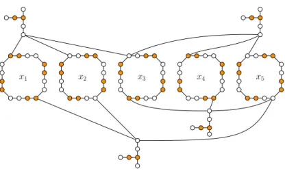
First, find and fix a planar embedding d of G(\phi ). G1(\phi ) is constructed from G(\phi )
and d as follows: For every variable xi, there is a cycle Zi = (zi,1, . . . , zi,12) of length
12. The vertices zi,1, zi,4, zi,7, zi,10 are referred to as true vertices of Zi; all other
vertices are false vertices. Moreover, vertices zi,1, zi,2, zi,3 are called upper vertices
of Zi, and vertices zi,7, zi,8, zi,9 are called lower vertices of Zi. Additionally, vertices
zi,4, zi,5, zi,6 are called right vertices of Zi, and zi,10, zi,11, zi,12 are called left vertices
of Zi.
For each clause cj, there is a cycle (cj,1, . . . , cj,4) of length 4 in G1(\phi ). To each
variable xi for i\in \{ 2, . . . , n - 1\} , we associate two disjoint sequences Ui =\bigl( uj\bigr)
| Ui|
j=1 and Li = \bigl( lj\bigr)
| Li|
j=1 of clauses xi appears in. The sequences are constructed using
a clockwise (with respect to d) enumeration of the edges of xi in G(\phi ), starting
with xi - 1xi. Let (xi - 1xi, xicj1, . . . , xicj\lambda , xixi+1, xicj\lambda +1, . . . , xicj\mu ) be the sequence of
edges encountered in this manner, and set Ui:= (cj1, . . . , cj\lambda ) and Li:= (cj\lambda +1, . . . , cj\mu ).
For i\in \{ 1, n\} , Liis empty and Uicontains all clauses xi appears in, again in clockwise
order. In G1(\phi ), the clauses and variables are connected such that for each clause cj
that xi occurs in, either the upper or the lower true vertex of xi is adjacent to cj,1.
More precisely, for variable xi, if cj = um, we add the edge cj,1zi,1 to connect the
upper true vertex to the clause. If cj= lm, we add cj,1zi,7 to connect the lower true
vertex to the clause. Because the order of edges around each vertex is preserved by
the construction, the graph G1(\phi ) obtained in this way can be embedded in the plane
by a suitable adaptation of d. See Figure 2 for an example of the construction.
x1 x2 x3 x4 x5 c1 c2 c3 c4 z1,1 c1,1 c1,3 z1,3
Fig. 2. A formula graph G(\phi ) (dashed) and the corresponding G1(\phi ) (solid).
Now we prove that G1(\phi ) is conflict-free 1-colorable iff \phi is 1-in-3-satisfiable.
Regarding necessity, a valid truth assignment b : X \rightarrow \BbbB yields a valid conflict-free
coloring by coloring the vertex cj,3of every clause, coloring all true vertices of variables
with b(xi) = 1, and coloring the false vertices zi,3, zi,6, zi,9, zi,12of all other variables.
Thus, in every cycle Zi, every third vertex is colored, providing a conflict-free neighbor
to every vertex of Zi. Moreover, in each clause, by virtue of cj,3 being colored, vertices
cj,2, cj,3, cj,4 have a conflict-free neighbor. Because b is a valid truth assignment, for
each clause, the vertex cj,1 is adjacent to exactly one colored true vertex. Therefore,
the coloring constructed in this way is conflict-free.
Regarding sufficiency, we first argue that the vertices cj,1, cj,2, cj,4 can never be
colored: If cj,1 receives a color, then cj,3 still enforces that one of cj,2, cj,3, cj,4 is
colored, leading to a contradiction in either case. If cj,2 receives a color, then cj,4
cannot have a conflict-free neighbor and vice versa. Therefore, no clause vertex can
be the conflict-free neighbor of any vertex of Zi. Thus, the conflict-free neighbor of
every vertex of Zi must itself be a vertex of Zi. Moreover, the conflict-free neighbor of
every vertex cj,1 must be a true vertex. Thus, there are exactly three ways to color
each cycle Zi: either by coloring the true vertices (one possibility), or by coloring
every other false vertex (two possibilities). A valid conflict-free 1-coloring of G1(\phi )
satisfies the property that for each clause cj, exactly one of the true vertices adjacent
to cj,1 is colored. Hence, a valid conflict-free 1-coloring of G1(\phi ) induces a valid truth
assignment b by setting b(xi) = 1 iff all true vertices of xi are colored.
Theorem 4.2. It is NP-complete to decide whether a planar graph admits a
conflict-free2-coloring.
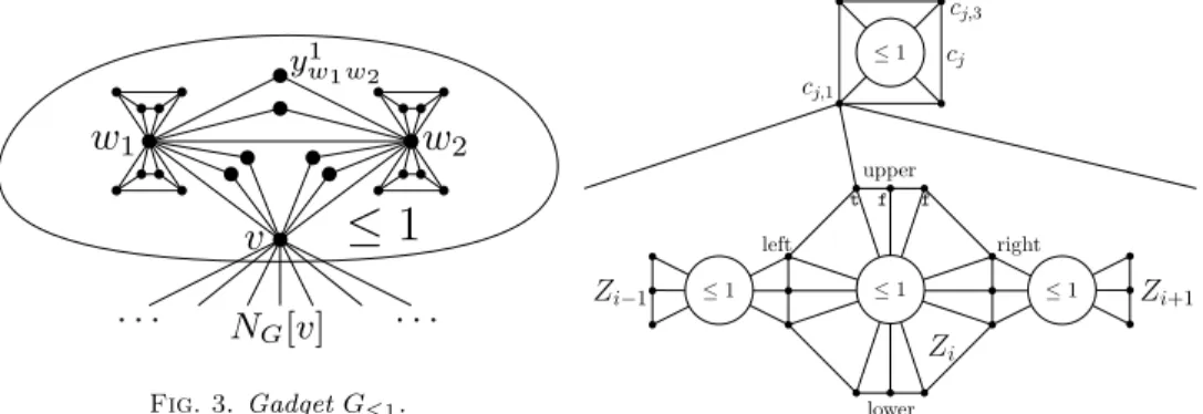
The proof requires the gadget G\leq 1 depicted in Figure 3. G\leq 1 consists of three
vertices v, w1, w2forming a triangle. Each edge ux of the triangle has two corresponding
vertices y1
ux, yux2 , each connected to u and x. Furthermore, both w1and w2are attached
to two copies of a cycle on four vertices, where every vertex of both cycles is adjacent
to the corresponding wi. G\leq 1 can be used to enforce that the vertices connected to
its central vertex v are colored using at most one distinct color.
Lemma 4.3. Let G = (V, E) be any graph, let v \in V , and let G\prime be the graph
resulting from adding a copy ofG\leq 1 toG by identifying v in G with v in G\leq 1. Then
(1) G\prime is planar ifG is, and (2) every conflict-free 2-coloring of G\prime leavesv uncolored
and uses at most one color onNG[v].
Proof. The planarity of G\prime follows from the planarity of G by the observation that
G\leq 1 is planar and can be embedded in any face incident to v in a planar embedding
of G. Now consider a conflict-free 2-coloring \chi of G\prime . \chi must color both w
1and w2.
Otherwise, \chi restricted to each of the two 4-cycles adjacent to wi must be a valid
conflict-free 2-coloring. However, as C4 requires at least two different colors, withen
sees two occurrences of both colors, and thus cannot have a conflict-free neighbor
anymore. Furthermore, \chi (w1)\not = \chi (w2), as otherwise y1w1w2 and y
2
w1w2 must both be
colored with the other color; but then, w1 and w2again see two occurrences of both
colors. By an analogous argument, \chi must not color v. Moreover, \chi cannot use more
than one color on NG[v], because v already sees one occurrence of each color, so adding
another occurrence of both colors would yield a conflict at v.
v
≤ 1
. . .
. . .
w
1w
2N
G[v]
yw11w2
Fig. 3. Gadget G\leq 1.
Zi ≤ 1 Zi+1 ≤ 1 ≤ 1 cj,3 cj,1 ≤ 1 cj Zi−1 upper lower left right t f f
Fig. 4. Clause and variable gadget for k = 2.
Proof of Theorem 4.2. NP-hardness is proven by constructing, in polynomial time,
a planar graph G2(\phi ) from the graph G1(\phi ) used in the hardness proof for k = 1, such
that G2(\phi ) is conflict-free 2-colorable iff G1(\phi ) is conflict-free 1-colorable.
The construction is carried out by adding a gadget G\leq 1 to every variable cycle Zi
of G1(\phi ), to every clause cycle, and between the right and left vertices of two adjacent
variable cycles Zi and Zi+1. This is depicted in Figure 4. More precisely, for every
cycle Zi, we add one copy of gadget G\leq 1and connect its central vertex v to all vertices
of the cycle. In a planar embedding of G2(\phi ), these gadgets can be embedded within
the face defined by the cycles Zi and thus do not harm planarity. By Lemma 4.3, this
enforces that on every cycle, only one color can be used. Moreover, for every edge
xixi+1 in G(\phi ), we add one copy of G\leq 1 that we connect to the right vertices of xi
and the left vertices of xi+1. This preserves planarity because these gadgets and the
added edges can be embedded in the face crossed by xixi+1 in some fixed embedding
d of G(\phi ). As one of the right vertices of xi and one of the left vertices of xi+1 must
be colored, this enforces that the same single color must be used to color all cycles Zi.
Finally, we add a copy of G\leq 1 to every clause cj and connect it to cj,1, . . . , cj,4. Again,
this preserves planarity because the gadget may be embedded in the face defined by (cj,1, . . . , cj,4).
We now argue that G2(\phi ) is conflict-free 2-colorable iff G1(\phi ) is conflict-free
1-colorable. A 1-coloring of G1(\phi ) induces a 2-coloring of G2(\phi ) by copying the color
assignment and coloring the internal vertices of the added gadgets as described in
the proof of Lemma 4.3. Now, let G2(\phi ) be conflict-free 2-colorable and fix a valid
2-coloring \chi . In each clause, \chi must color cj,3 and neither cj,1, nor cj,2, nor cj,4 can
be colored. Therefore, no clause vertex can be the conflict-free neighbor of any vertex
of Zi. Thus, the conflict-free neighbor of every vertex of Zi must itself be a vertex of
Zi. Moreover, the conflict-free neighbor of every vertex cj,1 must be a true vertex. As
there is only one color available to color all cycle vertices of all variables, the restriction
of \chi to the vertices of G1(\phi ) yields a valid 1-coloring except for the fact that some cj,3
might use a different color than the one used for the variables. However, this can be
fixed by simply replacing all occurring colors with one single color. Hence, G2(\phi ) is
conflict-free 2-colorable iff G1(\phi ) is conflict-free 1-colorable.
4.2. Sufficient number of colors. As shown above, it is NP-complete to decide
whether a planar graph has a conflict-free k-coloring for k\in \{ 1, 2\} . On the positive
side, we can establish the following result, which follows from the more general results discussed in section 3.2.
Corollary 4.4 (of Theorem 3.5). Every outerplanar graph is conflict-free
2-colorable, and every planar graph is conflict-free3-colorable. Moreover, such colorings
can be computed in polynomial time.
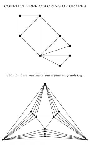
Outerplanar graphs are not the only interesting graph class for which one might suspect two colors to be sufficient. Two other interesting subclasses of planar graphs are series-parallel graphs and pseudomaximal planar graphs. However, each of these
classes contains graphs that do not admit a conflict-free 2-coloring: The graph G3
as defined in section 3 is an example of a series-parallel graph requiring three colors.
Figure 5 depicts a maximal outerplanar graph O9 satisfying \chi CF(O9) = 2. This graph
can be used to obtain a pseudomaximal planar graph M with \chi CF(M ) = 3 by adding
two copies of O9 to the neighborhood of every vertex of a triangle, similar to the
construction of G3, and adding gadgets on the inside of the triangle as depicted in
Figure 6.
Furthermore, observe that Theorem 4.4 does not hold if every vertex must be colored. In this case, there are outerplanar graphs requiring 3 colors for a conflict-free
Fig. 5. The maximal outerplanar graph O9.
Fig. 6. The pseudomaximal planar graph M , without the O9 gadgets.
coloring. One can obtain an example of such a graph by adding a chord to a cycle of length 5.
5. Closed neighborhoods: Planar conflict-free domination. In this
sec-tion we consider the decision problem k-Conflict-Free Dominating Set for planar
graphs. In section 5.1, we deal with the cases when k \in \{ 1, 2\} for planar and
out-erplanar graphs, and we give a polynomial-time algorithm to compute an optimal
conflict-free coloring of outerplanar graphs with k\in \{ 1, 2\} colors. Section 5.2 discusses
the problem for k\geq 3.
5.1. At most two colors. We start by pointing out that, for every conflict-free
1-colorable graph G, \gamma 1
CF(G) = \gamma (G) holds. Moreover, Corollary 5.1 discusses the
complexity of k-Conflict-Free Dominating Set, and Theorem 5.2 states positive results for outerplanar graphs.
Corollary 5.1 (of Theorems 4.1 and 4.2). k-Conflict-Free Dominating
Set is NP-complete for k\in \{ 1, 2\} for planar graphs.
Theorem 5.2. Let k\in \{ 1, 2\} , and let G be an outerplanar graph. We can decide
in polynomial time whether\chi CF(G)\leq k. Moreover, we can compute a conflict-free
k-coloring of G that minimizes the number of colored vertices in\scrO (n4k+1) time.
The proof of Theorem 5.2 relies on a polynomial-time algorithm that computes a k-coloring of the input outerplanar graph G if and only if such a coloring exists.
Intuitively speaking, our algorithm works as follows. For each vertex v \in G and
each edge vw\in G, we consider all possible assignments of conflict-free neighbors to v
and w and colors to these conflict-free neighbors. Each such assignment is called a
neighborhood configuration. Because the number of colors is constant and there is at most one conflict-free neighbor per color for each vertex, there are only polynomially many neighborhood configurations for each vertex or edge.
s w v V2 V1 N [s]
(a) An outerplanar graph G and an edge separator s = \{ v, w\} splitting G into components V1 and V2with a
neighbor-hood configuration of s (white and gray vertices). G[V2∪ s] w v G[V1∪ s] w v
(b) Colorings extending the neighborhood config-uration of s. These colorings are conflict-free on V1and V2 and can be combined to a conflict-free
coloring of G. Note that v /\in V1 does not need to
have a conflict-free neighbor in the coloring of V1.
Fig. 7. If we fix a neighborhood configuration of a separator of G and find conflict-free colorings of the separated components that extend this neighborhood configuration, we can combine these colorings to a conflict-free coloring ofG.
We decompose the outerplanar input graph at vertex separators (articulation points) and edge separators (edges shared by faces); removing the vertices of a separator splits the graph into several components. The following key property of this decomposition is the basis for our dynamic programming algorithm; see Figure 7. Let
s be a separator in our graph, and let V1, . . . , Vk be the vertex sets of the components
of G after removing s. If we fix a neighborhood configuration\scrC of s and find, for each
component G[Vi\cup s], a coloring extending \scrC that is conflict-free on Vi, then we can
combine these colorings to a coloring of G.
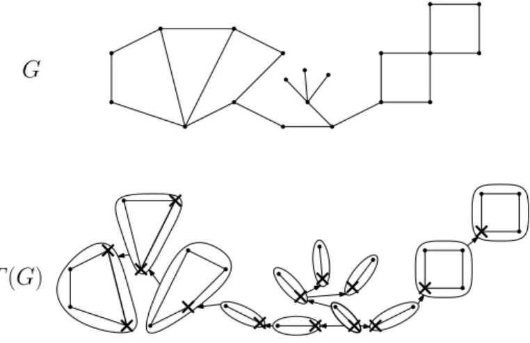
G
T (G)
Fig. 8. The arborescence T (G) (bottom) for an outerplanar graph G (top). The vertices of the incoming separator of each atom are marked \times ; incoming edge separators are drawn in bold. The root atom is drawn with bold outline and has an arbitrarily chosen vertex as incoming separator.
Our decomposition yields an arborescence of components as depicted in Figure 8, with edges between components that share a separator, using an arbitrary component
as root and directing all edges accordingly. In this arborescence, each component except the root has a unique incoming edge corresponding to a separator, called the
incoming separator of the component marked\times in Figure 8. Starting at the leaves,
we use dynamic programming on this arborescence as follows. For each component and each possible neighborhood configuration of the incoming separator, we compute a conflict-free k-coloring that extends the neighborhood configuration and minimizes the number of colored vertices, or find that this neighborhood configuration does not allow a conflict-free k-coloring. At the root, this allows us to determine whether the graph is conflict-free k-colorable. Moreover, if the graph is colorable, we can retrieve a coloring that minimizes the number of colored vertices. In the following, we give a detailed formal description of this algorithm, prove its correctness, and analyze its runtime.
5.1.1. Preliminaries. Let G = (V, E) be an outerplanar graph. W.l.o.g., we
assume that G is connected and has at least two vertices. Let \chi : V\prime \subseteq V (G) \rightarrow
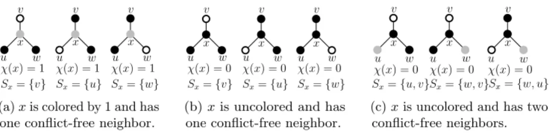
\{ 0, 1, . . . , k\} be a partial coloring of the vertices of G, and let v \in V . Observe that \chi defined like this modifies the definition given in the introduction by assigning color 0 to uncolored vertices. We begin by defining vertex neighborhood configurations. Intuitively speaking, a vertex neighborhood configuration assigns a color to v and lists all conflict-free neighbors of v together with their color; see Figure 9. In Figures 9, 10, and 11, black disks correspond to uncolored vertices, gray disks correspond to vertices colored by 1, and empty disks correspond to vertices colored by 2.
u v w x u v w x u v w x χ(x) = 1 χ(x) = 1 χ(x) = 1 Sx={v} Sx={u} Sx={w} (a) x is colored by 1 and has one conflict-free neighbor.
u v w x u v w x u v w x χ(x) = 0 χ(x) = 0 χ(x) = 0 Sx={w} Sx={v} Sx={u}
(b) x is uncolored and has one conflict-free neighbor.
u v w x u v w x u v w x χ(x) = 0 χ(x) = 0 χ(x) = 0 Sx={u, v}Sx={w, v}Sx={w, u} (c) x is uncolored and has two conflict-free neighbors. Fig. 9. A vertex x with three neighbors and the possible neighborhood configurations of s, modulo switching labels of the colors.
Definition 5.3 (vertex neighborhood configuration). A vertex neighborhood
configuration is a tuple\scrC v= [\chi (v), Sv, \rho v], where \chi (v)\in \{ 0, 1, . . . , k\} denotes the color
of v; if \chi (v) = 0, we regard v as uncolored; see Figure 9. The set \emptyset \not = Sv \subseteq N[v]
contains all conflict-free neighbors of v. Because there is at most one conflict-free
neighbor for each color,Sv contains at mostk elements. Finally, \rho v: Sv \rightarrow \{ 1, . . . , k\}
is an injective assignment of colors to the conflict-free neighbors ofv such that v\in Sv
implies\chi (v) = \rho v(v).
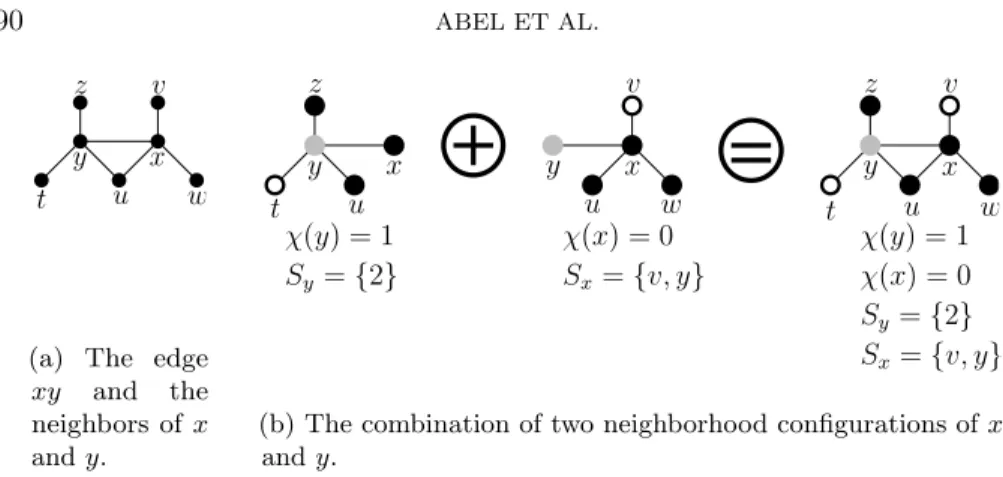
We call two vertex neighborhood configurations\scrC u,\scrC v for adjacent vertices u and
v compatible if they do not contradict each other in the following sense; see Figure 10. First, they must not assign different colors to the same vertex. Second, after combining
the partial colorings induced by \scrC u and \scrC v, all conflict-free neighbors specified in
the neighborhood configurations must remain conflict-free. An edge neighborhood configuration consists of two compatible vertex neighborhood configurations for its endpoints. Formally, we define this as follows.
u v w x y t z
(a) The edge xy and the neighbors of x and y. u v w x y t z u x y t z u v w x y χ(y) = 1 χ(x) = 0 χ(y) = 1 χ(x) = 0 Sy ={2} Sx={v, y} Sx={v, y} Sy={2}
(b) The combination of two neighborhood configurations of x and y.
Fig. 10. The combination of two neighborhood configurations of two adjacent vertices x and y results in a neighborhood configuration of the edgexy.
Definition 5.4 (edge neighborhood configuration). For an edge uv, we say that \scrC u= [\chi (u), Su, \rho u] and\scrC v= [\chi (v), Sv, \rho v] are compatible, denoted by \scrC u\updownarrow \scrC v, if the
following conditions hold; see Figure 10.
1. For every w\in Sv\cap Su, \rho u(w) = \rho v(w). If u is in Sv, then\chi (u) must be \rho v(u), and vice versa.
2. The combined coloring
\rho uv: Su\cup Sv\cup \{ u, v\} \rightarrow \{ 0, . . . , k\} , w \mapsto \rightarrow \left\{
\chi (w) ifw\in \{ u, v\} , \rho u(w) ifw\in Su,
\rho v(w) otherwise
must be injective onN [v] and N [u], with the exception that both u and v may
receive color0.
An edge neighborhood configuration of e = uv is a pair \scrC e= [\scrC u,\scrC v] of compatible
vertex neighborhood configurations. Forw\in \{ u, v\} , \scrC w
e shall denote the neighborhood
configuration ofw contained in \scrC e.
Observe that we can check in\scrO (k) time whether a pair of vertex neighborhood
configurations is compatible. For a pair of incident edges, we call a pair of edge neighborhood configurations compatible if the neighborhood configuration of v is the same in both neighborhood configurations; see Figure 11.
u v w x y t s z q r
(a) Two adjacent edges yx and xz and the neigh-bors of y, x, and z. u v w x y t z χ(y) = 1 χ(x) = 0 Sx={v, y} u v x w s z y r q χ(x) = 0 Sx={v, y} χ(z) = 0 Sz={q, r} u v w x y t s z Sy={t} q r χ(y) = 1 χ(x) = 0 χ(z) = 0 Sy={t} Sx={v, y} Sz={q, r}
(b) Two compatible neighborhood configurations of the two adjacent edges yx and xz.
Fig. 11. Compatible neighborhood configurations of adjacent edges.
Definition 5.5 (compatibility). If \scrC ev = \scrC ev\prime for a pair e = uv, e\prime = vw of
incident edges, then we say\scrC e\prime is compatible with\scrC e; see Figure 11.
We observe that if we have a neighborhood configuration for each edge and all these neighborhood configurations are pairwise compatible, the colors of all vertices are fixed in a consistent manner, and we can thus derive a conflict-free k-coloring from the neighborhood configurations.
Observation 5.6. Let\scrC be a set of edge neighborhood configurations containing
one neighborhood configuration\scrC efor each edge e. If\scrC eand\scrC e\prime are compatible for
every pair e = uv, e\prime = vw of incident edges, a conflict-free k-coloring can be obtained
from\scrC .
Our algorithm works by dynamic programming on an arborescence T (G) derived from a decomposition of G along vertex separators and edge separators into components called atoms.
Definition 5.7. A vertex separator of G is an articulation point of G, i.e., a
vertex whose removal disconnectsG. An edge separator of G is an edge uv of G such
that removingu and v disconnects G. An atom of G is either an edge atom (formed
by an edge) or a face atom (induced chord-free cycle ofG).
Observe that, because G is outerplanar, any connected induced subgraph of G with at least two vertices either is an atom or contains a separator. The vertex set V (T (G)) of the arborescence T (G) consists of atoms of G and is defined by induction
on the induced subgraphs G\prime of G as follows. If an induced subgraph G\prime of G is an
atom, V (T (G\prime )) =\{ G\prime
\} . If G\prime is no atom, let s =
\{ v\} be a vertex separator of G\prime if
one exists; otherwise, let s =\{ u, v\} be an edge separator of G\prime . Let V\prime
1, . . . , V\ell \prime be the
vertex sets of the connected components of G\prime
- s, and let G\prime
1, . . . , G\prime \ell be the subgraphs
induced by V\prime
1\cup s, . . . , V\ell \prime \cup s. Then V (T (G\prime )) = \bigcup
1\leq i\leq \ell V (T (G\prime i)) is the set of all
atoms obtained by further subdividing G\prime .
There is an arc between two vertices of T (G) if the two atoms share a separator. To avoid cycles in T (G), if more than two atoms share a vertex separator, instead of introducing an arc between every pair of them, we pick an arbitrary atom among them and connect it to all other atoms sharing the vertex separator. Because G is outerplanar, this yields a tree of atoms of G; we turn this tree into the arborescence T (G) by picking an arbitrary root vertex and orienting all edges away from this root. Each vertex a of T (G) except for the root has a unique incoming arc corresponding to a unique separator, called the incoming separator of the atom a. For the root atom r, we pick an arbitrary vertex of r as incoming separator; in this way, each
atom a has exactly one incoming separator sa. See Figure 8 for an example of the
construction. For an atom a\in T (G), we denote by T (G, a) the subtree of T (G) rooted
at a. Moreover, let S(G, a) be the subgraph of G induced by all vertices occurring in any atom in T (G, a).
5.1.2. Description of the algorithm. For each vertex and each edge, our
algorithm keeps a list of feasible neighborhood configurations. At any point in the algorithm, we know that any neighborhood configuration not on this list cannot be extended to a conflict-free k-coloring of G. Whenever we remove a neighborhood configuration from the list of feasible neighborhood configurations for a vertex, we also remove all corresponding neighborhood configurations from its incident edges. Similarly, when we remove the last neighborhood configuration of an edge that contains a certain vertex neighborhood configuration, we also remove that neighborhood configuration
from the list of feasible neighborhood configurations of the vertex. In this way, deleting a feasible neighborhood configuration may cause a cascade of further deletions; however,
a careful implementation of our algorithm can handle these deletions in \scrO (1) time
per deleted neighborhood configuration. Because each neighborhood configuration is deleted at most once, this does not affect our asymptotic running time.
e1 e2 e3 e4 e5 e6 Gf f
(a) A neighborhood con-figuration of a face f of G. Ce1 Ce2 Ce3 Ce4 Ce5 Ce6 T2 T3 T4 T5 T6 Df
(b) The neighborhood configuration graph of f and the cycle in the neighborhood configuration graph corresponding to the neighborhood configuration of Figure 12a.
Fig. 12. A face of G and the corresponding neighborhood configuration graph.
We initialize the lists of feasible neighborhood configurations by computing, for each vertex and each edge, the list of all possible neighborhood configurations according
to Definitions 5.3 and 5.4. We proceed by refining, for each atom a\in V (T (G)), the
list of feasible neighborhood configurations of the incoming separator sa. This process
starts in the leaves of T (G) and works its way up towards the root, terminating once
the root has been processed. Processing an atom a\in V (T (G)) means removing all
neighborhood configurations\scrC sa of its incoming separator that cannot be extended
to a conflict-free k-coloring of S(G, a). Note that in this conflict-free k-coloring, the
vertices of sa need not have conflict-free neighbors in S(G, a) if\scrC sa is such that all
their conflict-free neighbors are outside of S(G, a). Moreover, for each atom a and
each feasible neighborhood configuration\scrC sa, the algorithm computes and stores the
minimum number of colored vertices required for a conflict-free k-coloring of S(G, a) extending\scrC sa.
If the list of feasible neighborhood configurations of any vertex or edge becomes empty at any point, the algorithm aborts and reports that the graph is not conflict-free k-colorable. Otherwise, after processing the root r, the algorithm checks all feasible
neighborhood configurations of srto find a neighborhood configuration for which the
number of colored vertices is minimal. Starting with this neighborhood configuration,
the algorithm backtracks and reconstructs a conflict-free k-coloring of G with a minimal number of colored vertices.
It remains to describe how to process an atom of T (G). In case of a face atom f , the incoming separator can be either a vertex separator or an edge separator.
We assume that it is an edge separator e1 = uv; vertex separators can be handled
analogously. The face f may contain vertices and edges that are not part of any separator. For those vertices and edges, we have already computed the set of feasible neighborhood configurations in the first step of the algorithm. All other vertices and edges except for the incoming separator correspond to children of f in T (G); therefore, we have already computed the set of feasible neighborhood configurations for each of them.
For each neighborhood configuration\scrC e1 still in the list of feasible neighborhood
configurations of e1, we build the directed neighborhood configuration graph G\ast =
(V\ast , E\ast ) as depicted in Figure 12b.
The vertex set of G\ast consists of the neighborhood configuration
\scrC e1 and each
feasible neighborhood configuration\scrC ei of each edge ei \not = e1 of f . There is an edge
between two neighborhood configurations\scrC uv,\scrC vw iff they are compatible. We choose
a direction of the edges around the face and direct all edges in G\ast accordingly; see
Figure 12b. Each simple directed cycle Df in G\ast must contain\scrC e1 and thus corresponds
to a selection of one neighborhood configuration for each edge of f ; these neighborhood configurations are pairwise compatible. Therefore, there is a conflict-free k-coloring of
S(G, f ) extending\scrC e1 iff there is a simple directed cycle in G
\ast .
Moreover, we add weights to the edges of G\ast such that the weight of a simple
directed cycle corresponds to the minimum number of colored vertices in such a coloring. In order to compute the weights, for vertices and edges of f that are separators corresponding to children of f in T (G), we make use of the minimum number of colored vertices in their corresponding subtrees that we computed earlier.
We can find a minimum-weight cycle in G\ast or decide there is no such cycle in
time\scrO (| V\ast | + | E\ast
| ), using an algorithm similar to Dijkstra's shortest path algorithm. We can do this in linear time because we can expand the vertices in fixed order, expanding all vertices corresponding to an edge of f before moving on to all vertices of the next edge around the face. If our algorithm finds a minimum-weight cycle, we store its weight as the minimum number of vertices colored in any conflict-free
k-coloring of S(G, f ) extending \scrC e1. Otherwise, \scrC e1 is removed from the list of
feasible neighborhood configurations of e1. Repeating this procedure for each feasible
neighborhood configuration of e1 concludes the processing of a face atom f .
In the following, we describe how to handle an edge atom e \in V (T (G)). In
this case, the incoming separator seis a vertex separator v. For each neighborhood
configuration in the list of feasible neighborhood configurations of v, there is at least one neighborhood configuration in the list of feasible neighborhood configurations of e; otherwise, we would have already deleted the neighborhood configuration. To compute the minimum number of colored vertices in S(G, e) for some neighborhood
configuration \scrC v, we check for each neighborhood configuration of e containing\scrC v,
the minimum number of colored vertices, taking into account the color of u and the minimum number of vertices computed for the children of e in T (G). Repeating this for each feasible neighborhood configuration of v concludes the processing of an edge atom e.
5.1.3. Correctness of the algorithm. Next, we argue that our algorithm is
correct, i.e., it finds a conflict-free k-coloring with minimum number of colored vertices
iff one exists. In this section, we call a neighborhood configuration valid if it can be extended to a conflict-free k-coloring of G.
There are only two reasons for deleting a neighborhood configuration \scrC from a
list of feasible neighborhood configurations. In the first case, the deletion of\scrC is a
consequence of a deletion of another neighborhood configuration\scrC \prime . In this case,
\scrC is
deleted because deleting\scrC \prime has led to an incident vertex or edge without a feasible
neighborhood configuration compatible to\scrC . This can never cause a valid neighborhood
configuration to be deleted unless we deleted a valid neighborhood configuration\scrC \prime
first.
In the second case, the deleted neighborhood configuration \scrC belongs to an
incoming separator sf of a face atom f for which the algorithm finds that there is
no conflict-free k-coloring of S(G, a) extending it. By induction on T (G), we assume that when we start processing f , no valid neighborhood configurations have been deleted from the list of feasible neighborhood configurations for any vertex or edge
of f . Assume there was a valid neighborhood configuration \scrC of sf deleted by our
algorithm. Because\scrC is valid, there is a conflict-free k-coloring of S(G, f) extending
\scrC . This yields a set of compatible neighborhood configurations for the edges of f
and thus a cycle in the corresponding neighborhood configuration graph G\ast . This is
a contradiction, because the algorithm only deletes \scrC if there is no such cycle. We
conclude that no valid neighborhood configuration is ever deleted from the list of feasible neighborhood configurations of any vertex or edge. Therefore, the algorithm will always find the graph to be conflict-free k-colorable if it is. In a similar manner, we can argue that the number of colored vertices used by the coloring produced by our algorithm is minimal.
In the remainder of the section, we prove that our algorithm never produces an invalid conflict-free k-coloring of G. Again, the proof is by induction on T (G). We discuss an inductive step for the case that the current atom is a face f with an
incoming edge separator e1; the induction base and the remaining cases are analogous.
We assume by induction that for each neighborhood configuration\scrC sa of the incoming
separator sa of each child a of f , there is a conflict-free k-coloring of S(G, a) extending
\scrC sa. Let \scrC be a neighborhood configuration of e1 that remains feasible after the
processing of f . This is because there is a cycle in the corresponding neighborhood
configuration graph G\ast . This cycle corresponds to a set of pairwise compatible edge
neighborhood configurations. We can construct a conflict-free k-coloring of S(G, f ) by combining the colorings induced by these neighborhood configurations and the corresponding colorings of the graphs S(G, a) for children a of f . At the root r of T (G), this yields a conflict-free k-coloring of G, because all neighbors of the incoming separator of r are part of S(G, r) = G. Therefore, our algorithm never produces an invalid conflict-free coloring.
5.1.4. Runtime of the algorithm. Finally, we need to analyze the running
time of our dynamic programming approach. We begin by observing that T (G)
has \scrO (n) atoms. Moreover, we observe that the number of vertex neighborhood
configurations \scrC v = [\chi (v), Sv, \rho v] of a vertex v is in \scrO (nk), as there are at most
\bigl( | N [v]|
k \bigr) \cdot k! possibilities for Sv and \rho v. Therefore, the number of edge neighborhood
configurations\scrC e= [\scrC u,\scrC v] of an edge e\in E is in \scrO (n2k).
Let f = e1e2. . . em be a face atom; the running time for processing face atoms
dominates the running time for all other computation steps of the algorithm. For f ,
we build the neighborhood configuration graph G\ast that has
\scrO (n2k+1) vertices, because
f has at most n edges, each with\scrO (n2k) neighborhood configurations. The number of
edges between the neighborhood configurations of two incident edges ei= uv, ei+1= vw
along f is at most\scrO (n3k) because there are only
\scrO (nk) neighborhood configurations
for each of the vertices u, v, and w. Therefore, the number of edges in G\ast is
\scrO (n3k+1).
This leads to a running time of \scrO (n5k+2), because we run a graph scan on G\ast for each
of the\scrO (n2k) neighborhood configurations of the incoming separator and each of the
\scrO (n) face atoms.
Streamlining this approach leads to a runtime of \scrO (n4k+1). In particular, we
modify our subroutine processing a face atom f that has an incoming edge separator
e = uv as follows. For each neighborhood configuration \scrC v of v we extend the
neighborhood configuration graph G\ast of f by considering all feasible neighborhood
configurations \scrC e1 of e1 such that \scrC
v
e1 = \scrC v holds and compute minimum-weight
cycles in G\ast . For each neighborhood configuration\scrC e1 of e1 that is reached during an
application of the shortest path algorithm, we obtain the minimum number of vertices
colored in any conflict-free coloring of S(G, f ) extending \scrC e1. As the number of all
edge and vertex neighborhood configurations of G is\scrO (n3k+1), we obtain an overall
runtime of\scrO (n4k+1).
This concludes the proof of Theorem 5.2.
5.2. Approximability for three or more colors. In section 4.2 we stated that
every planar graph is conflict-free 3-colorable. In this section we deal with conflict-free 3-colorings of planar graphs that, additionally, minimize the number of colored vertices.
Theorem 5.8. Let k\geq 3, and let G be a planar graph. The following hold:
(1) Unless P = NP, there is no polynomial-time approximation algorithm providing
a constant-factor approximation of\gamma 3
CF(G) for planar graphs.
3-Conflict-Free Dominating Set is NP-complete for planar graphs.
(2) For k \geq 4, k-Conflict-Free Dominating Set is NP-complete. Also,
\gamma k
CF(G) = \gamma (G), and the problem is FPT with parameter \gamma CFk (G).
Further-more, there is a PTAS for\gamma k
CF(G).
(3) If G is outerplanar, then \gamma k
CF(G) = \gamma (G), and there is a linear-time algorithm
to compute \gamma k
CF(G).
The proof of Theorem 5.8 is based on the following polynomial-time algorithm, which transforms a dominating set D of a planar graph G into a conflict-free k-coloring of G, coloring only the vertices of D: Let D be a dominating set of a planar graph
G. Every vertex v\in V (G) \setminus D is adjacent to at least one vertex in D. Pick any such
vertex u\in D and contract the edge uv \in E(G) towards u. Repeat this until only the
vertices from D remain. Because G is planar, the graph G\prime = (D, E\prime ) obtained in this
way is planar, as G\prime is a minor of G. By the 4-coloring theorem, we can compute a
proper 4-coloring of G\prime .
Lemma 5.9. The 4-coloring generated by this procedure induces a conflict-free 4-coloring of G.
Proof. Every vertex u\in D is a conflict-free neighbor to itself as its color does not
appear in NG(u). Let v\in V (G) \setminus D be some uncolored vertex, and let u \in D be the
vertex that v was contracted towards by the algorithm. In G\prime , this contraction made
u adjacent to all other vertices in NG(v)\cap D, which guarantees that the color of u is
unique in NG(v)\cap D. As V (G) \setminus D remains uncolored, the color of u is thus unique in
NG[v].
Proof of Theorem 5.8. Proposition (1) follows from Theorem 3.7 of section 3.3:
The reduction used there preserves planarity and proper planar 3-coloring is