HAL Id: hal-03164528
https://hal.uca.fr/hal-03164528
Submitted on 10 Mar 2021
HAL is a multi-disciplinary open access
archive for the deposit and dissemination of sci-entific research documents, whether they are pub-lished or not. The documents may come from teaching and research institutions in France or abroad, or from public or private research centers.
L’archive ouverte pluridisciplinaire HAL, est destinée au dépôt et à la diffusion de documents scientifiques de niveau recherche, publiés ou non, émanant des établissements d’enseignement et de recherche français ou étrangers, des laboratoires publics ou privés.
Thermal conductivities of solid and molten silicates:
Implications for dynamos in mercury-like proto-planets
D. Freitas, J. Monteux, Denis Andrault, Geeth Manthilake, A. Mathieu,
Federica Schiavi, N. Cluzel
To cite this version:
D. Freitas, J. Monteux, Denis Andrault, Geeth Manthilake, A. Mathieu, et al.. Thermal conductivities of solid and molten silicates: Implications for dynamos in mercury-like proto-planets. Physics of the Earth and Planetary Interiors, Elsevier, 2021, 312, pp.106655. �10.1016/j.pepi.2021.106655�. �hal-03164528�
1
Thermal conductivities of solid and molten silicates: implications for
1
dynamos in Mercury-like proto-planets
23
D. Freitas1,$*, J. Monteux1, D. Andrault1, G. Manthilake1, A. Mathieu1, F. Schiavi1, N. Cluzel1 4
5
1Université Clermont Auvergne, CNRS, IRD, OPGC, Laboratoire Magmas et Volcans, F-6300 6
Clermont-Ferrand, France 7
$Now at School of Geosciences, Grant Institute, The King’s Buildings, The University of 8
Edinburgh, West Mains Road, Edinburgh EH9 3JW, United Kingdom 9
10 11
*Corresponding Author: Damien Freitas ([email protected])
12 13 14 Abstract 15 16
Remanent magnetization and active magnetic fields have been detected for several telluric 17
planetary bodies in the solar system (Earth, Mercury, Moon, Mars) suggesting the presence of core 18
dynamos active at the early stages of the planet formation and variable lifetimes. Among the factors 19
controlling the possibility of core dynamos generation, the dynamics of the surrounding silicate 20
mantle and its associated thermal properties are crucial. The mantle governs the heat evacuation from 21
the core and as a consequence the likeliness of an early thermally driven dynamo. In the case of 22
planets with a thick mantle (associated with supercritical Rayleigh numbers), the core heat is 23
efficiently removed by mantle convection and early thermally-driven dynamos are likely. At the 24
opposite, planets with a thin mantle (associated with subcritical Rayleigh numbers) might evacuate 25
their inner heat by diffusion only, making early thermally-driven dynamos difficult. Within the Solar 26
System, Mercury is a potential example of such a regime. Its small mantle thickness over the planet 27
radius ratio might be inherent to its small orbital semi-axis and hence, might be ubiquitous among the 28
terrestrial objects formed close to their star. 29
To constrain the likeliness of a thermally driven dynamo on “Mercury-like” planets (i.e. with 30
large Rc/R), we present new thermal diffusivity measurements of various solid, glassy and molten 31
samples. We applied the Angstrom method on cylindrical samples during multi-anvil apparatus 32
experiments at pressures of 2 GPa and temperatures up to 1700 K. Thermal diffusivities and 33
conductivities were estimated for solid and partially molten peridotites, with various melt fractions, 34
and for basaltic and rhyolitic glasses and melts. Our study demonstrates that melts have similar 35
thermal properties despite a broad range of composition investigated. The melts reveal much lower 36
thermal conductivities than the solids with almost an order of magnitude of decrease: 1.70 (±0.19) to 37
2.29 (±0.26) W/m/K against 0.18 (±0.01) to 0.41 (±0.03) W/m/K for peridotites at high temperatures 38
and various melts respectively. Partially molten samples lie in between and several predictive laws 39
are proposed as a function of the melt fraction and solid/melt texture. 40
Using our results into forward calculations of heat fluxes for dynamo generation for Mercury-41
like planets, we quantify the effect of mantle melting on the occurrence of thermally driven dynamos. 42
The presence of a mushy mantle and partial melting could significantly reduce the ability of the 43
mantle to evacuate the heat from the core and can prevent, shut or affect the presence of a planetary 44
magnetic field. The buoyancy and fate of molten material in such bodies can thus influence the 45
magnetic history of the planet. Future observations of Mercury-like planets accreted near their star 46
and the detections of their magnetic signatures could provide constraints on their inner state and 47
partial melting histories. 48
49
Keywords: Thermal diffusivity; thermal conductivity; melts; geodynamo; Mercury;
50
2 51
Author contributions:
52
GM, AM, DA and DF set up the MAA apparatus and heating system for Angström measurements. 53
DF and GM conceived the experiments. DF performed, processed and analyzed the experiments. FS 54
significantly contributed to Raman micro-analyses. NC helped for sample selections, analyses and 55
preparations prior experimental runs. JM, DA, GM and DF realized the modelling and discussion 56
section. DF, JM and DA wrote the manuscript. All of the authors have agreed and contributed to the 57 manuscript. 58 59 60 Introduction 61 62
The presence of internally generated magnetic fields is a variable feature among telluric bodies 63
in the inner solar system. While few are currently active, such as for Mercury and Earth, several are 64
now extinct, as observed for the Moon, Venus and Mars. On terrestrial planets currently exhibiting a 65
dynamo, the generated magnetic fields characteristics are very different. Earth’s magnetic field is 66
very intense 25-65 µT, originating from the core and present for at least 3.5 Ga (Tarduno et al. 2010). 67
Mercury’s field strength is much weaker, representing around a 1% of Earth’s one (Kabin et al. 2008; 68
Anderson et al., 2011) and its shape is also unique among the different detection in the solar system 69
(Tian et al., 2015). According to the remnant magnetization measured in the crust, it was proposed 70
that such weak magnetic activity occurred during the last 3.9 Ga (Johnson et al. 2015). The source of 71
such a weak-and-prolonged dynamo is still largely debated (Manthilake et al. 2019). In the meantime, 72
there are several evidences for an intrinsic dynamo during the early stages of both Mars and Moon 73
(Acuña et al., 1999; Hood et al., 2010). Their dynamo seems to cease around 4.1-3.9 Ga ago for Mars 74
(Johnson and Phillips, 2005; Lillis et al., 2008, Lillis et al., 2013) and exhibits a somewhat 75
complicated history for the Moon with a strong dynamo between 4.25 and 3.5 Ga, followed by a weak 76
persistence up to 2.5-2 Ga ago (Tikoo et al. 2014, Lawrence et al. 2008, Garrick-Bethell et al., 2009, 77
Mighani et al. 2020). For Venus, the early presence of a dynamo remains yet unconstrained but may 78
be detectable in future explorations (Nimmo et al. 2002; O’Rourke et al. 2019). More broadly, 79
evidences of paleomagnetic anomalies indicate that the angrite parent bodies, originating from inner 80
regions of the solar system, were subject to an early internally generated dynamo (Weiss et al. 2008). 81
All these elements suggest that transient dynamos might be a somewhat common feature in telluric 82
bodies (Monteux et al. 2011). 83
The presence of early dynamos is highly conditioned by the internal structure of the planet and 84
its capacity to release the heat accumulated during the accretion processes (accretion, metal/silicate 85
differentiation, core and mantle crystallization) as well as short-lived radiogenic heating. As heat 86
conduction is an inefficient heat transport process in silicates at high temperatures (Hofmeister and 87
Branlund, 2015), the onset of a mantle global convection is a crucial step in planet’s thermal history. 88
Convection starts when the Rayleigh number (Ra) of the terrestrial mantle is larger than the critical 89
Rayleigh number (Rac). The higher is Ra, the stronger the convection, and the more efficient the heat 90
transport. In contrast, heat is only transported by conduction for a terrestrial mantle with a Ra<Rac. 91
As Ra scales with mantle thickness (hmantle) as hmantle3, convection should take place easily in planets
92
with a thick silicate mantle, even after the solidification of the early magma ocean stage. 93
Consequences are efficient evacuation of the inner heat and the possible occurrence of a dynamo. At 94
the opposite, bodies with a thinner mantle lead to smaller Ra values, making convection unlikely and 95
dynamos more difficult to generate. 96
Mercury is the most interesting planet for our study. Indeed, its mantle is thin 420 ± 30 km (Hauck 97
et al. 2013) and its core occupies almost 55% of planet’s volume and 65% of the planet mass (Strom 98
and Spague, 2003; Charlier and Namur, 2019). Hence, the mantle of Mercury is controversially at the 99
limit between conductive and convective regimes (Breuer et al. 2007). Different scenarios could 100
3 explain the small hmantle/planet radius (R) ratio on Mercury (Charlier and Namur, 2019): (1) primordial 101
nebular processes, yielding to the enrichment of metal over silicate materials in the inner solar system 102
(Ebel and Grossman, 2000; Wurm et al. 2013; Weidenschilling 1978), (2) highly energetic accretional 103
collisions inducing a major loss of the silicate fraction (Benz et al. 1988, Asphaug and Reufer, 2014), 104
and (3) post–accretion scenarios, with major vaporization of the volatile and silicate elements from 105
the planet during magma ocean stage (Fegley and Cameron 1987; Boujibar et al., 2015). If scenarios 106
(1) and (3) are dominant, then "Mercury-like" planets with small hmantle/R ratio would be ubiquitous 107
within all planetary systems. Moreover, such a small ratio would be prevailing during the whole 108
accretionary processes. Mercury-like bodies could adopt a wide range of possible compositions 109
depending on their history. For example, bodies accreted from reduced enstatite and/or carbonaceous 110
bencubbinite chondrites (Malavergne et al. 2010) could present a mantle composition similar to 111
terrestrial lherzolite, but with a sulfur content potentially as high as 11 wt.% (Namur et al. 2016). 112
Accordingly, the diversity of the silicate samples found on Earth in the forms of rocks, melts and 113
glasses is a good proxy to decipher the properties of a range of mantle-relevant silicate compositions 114
on Mercury-like bodies. Depending on the planet size and the hmantle/R ratio, the internal pressure 115
ranges from a few MPa to several GPa. We note that extensive mantle melting likely occurred at 116
different stages of the history of such Mercury-like bodies. Major energy incomes are expected from 117
the vicinity to the young Sun (2500 to 3500 K according Charlier and Namur, 2019), internal energy 118
release (chemical and gravitational differentiation, core crystallization), and presence of short-period 119
radioactive elements (Al26, K40 etc.). The very high temperatures likely induce extensive melting of 120
the thin mantle up to the core-mantle boundary (CMB). 121
As mentioned above, dynamo generation could be difficult for Mercury-like planets, due to the 122
subcritical value of Ra possibly disabling mantle convection. In such case, heat transfer by conduction 123
would dominate the planet history and the thermal conductivity of the silicate mantle is a key 124
parameter governing the early core heat flow. Silicates thermal conduction properties are now well 125
characterized at ambient conditions (Hofmeister and Branlund, 2015). Among them, the most 126
common geological minerals were characterized in the forms of single crystal and polycrystalline 127
aggregates: olivine (Osako et al. 2004; Xu et al. 2004; Perterman and Hofmeister 2006; Gibert et al. 128
2005), periclase (Hofmeister and Branlund, 2015), feldspar (Pertermann et al. 2008; Hofmeister et al. 129
2009; Branlund and Hofmeister, 2012) and pyroxenes (Hofmeister 2012, Hofmeister and Pertermann 130
2008) as well as peridotite rocks (Gibert et al. 2005; Beck 1978), which have been extensively studied 131
due to their important geological implications. The thermal diffusivities of minerals are linked to the 132
characteristics of their lattice structure and modes of phonon generation and propagation as a function 133
of temperature. For silicates, lattice thermal diffusivities usually decrease with increasing temperature 134
following a 1/T dependence. At the opposite, the diffusivities increase while increasing pressure, 135
however, the temperature dependence is much greater than that of pressure over the considered ranges 136
for small planets. The resulting implication is that mantle rocks and minerals are poor thermal 137
conductors in planetary interiors. Recent measurements of thermal diffusivities of glasses and melts 138
at ambient pressure suggested that the non-crystalline silicates are even more insulating than the 139
minerals (Hofmeister et al. 2009, 2014, Romine et al. 2012). 140
Measurements of thermal diffusivities at relevant conditions of planetary mantles encompass 141
important difficulties, which were overcome by the use of different techniques (see Hofmeister and 142
Brandlund 2015 for a critical review). Measurements were reported over a wide P and T range for 143
large volume samples of olivine, periclase, bridgmanite using Angström or Pulse method in solid 144
pressure apparatus (Osako et al. 2004; Xu et al. 2004; Manthilake et al. 2011a and 2011b, Zhang et 145
al. 2019). Up to now, accurate measurements of geologically relevant silicate glass, partially molten 146
systems and melts at planetary interior conditions remain scarce if not absent. The available results 147
report a nearly flat evolution of thermal diffusivities with the temperature above 1000 K for silicates, 148
glass and melts (Hofmeister et al. 2014; Hofmeister and Banlund, 2015), suggesting that the 149
4 measurements above the melting temperature could be safely extrapolated to planetary P-T 150
conditions. 151
In this study, we aim at better constraining the thermal properties of Mercury–like protoplanets 152
where convection is unlikely and heat is mostly removed by diffusion. We perform HP-HT in situ 153
thermal diffusivities measurements of solid, partially molten and fully molten silicate for various 154
compositions in Multi-anvil apparatus and using Angström method. Then, we constrain the likeliness 155
of a thermally driven dynamo during the early stages of the evolution of a Mercury-like planet. We 156
consider a wide range of planet sizes (1 km < R < RMercury) and thermal states (with solid and partially 157
molten mantles) on the dynamo likeliness. 158
159 160
Experimental and analytical methods
161 162
High-pressure assemblies: 163
High-pressure and high-temperature experiments were performed using a 1500-ton Kawai type 164
Multi-anvil apparatus. All experiments were conducted at 2 GPa, based on a previous press-load vs 165
sample pressure calibration (Boujibar et al. 2014), providing an uncertainty of ~0.1 GPa at pressures 166
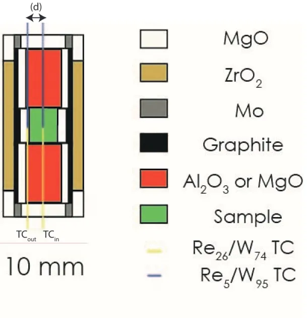
<5 GPa. We used octahedral pressure media with full length edges composed of MgO doped with 167
Cr2O3 (5 wt. %) in a 25/17 multi-anvil configuration (octahedron edge length / anvil truncation edge 168
length) (Figure 1). Our assembly was designed to accommodate the specific requirements for 169
measurements of thermal conductivity of relatively large samples (4 mm long for 4-3.5 mm diameter). 170
All ceramic parts of the cell assembly, including the pressure media, were fired at 1373 K prior 171
assembling in order to remove the absorbed moisture. Oxygen fugacity of the sample was not 172
controlled during the experiments but is expected to be quite reducing due to the presence of the 173
graphite furnace. The use of a steeped graphite furnace helped reducing thermal gradients. Thermal 174
loss from the sample zone was further reduced by the use of a thick zirconia (ZrO2) sleeve around the 175
furnace. Thermal gradients in our assembly were computed using the software developed by 176
Hernlund et al. 2006. The models show temperature gradients within the sample volume limited to 177
~7.5 K/mm vertically and even less radially/horizontally (Figure S1). On the other hand, uncertainties 178
of our thermocouple reading (i.e. where the conductivity measurement is performed, see below) are 179
less than 5 K on absolute and 0.1 K in relative temperatures. 180
Previous experimental studies described the difficulties to perform a good measurement of 181
thermal diffusivity for a molten sample, due to a potential sample deformation (Hofmeister et al. 182
2009, 2014; Romine et al. 2012). However, deformation remained minor in our experiments, as 183
evidenced by the good reproducibility of the measurements during the repeated cycles of heating and 184
cooling (Figures 1 and 2) as well as the shape of the recovered samples (Figures S6, S7 and S8). 185
Two tungsten-rhenium (W95Re5-W74Re26) thermocouples of 75 µm of diameter were used to 186
measure temperature oscillations at the center (in 300 and 600 µm drilled holes in solids and glasses, 187
respectively) and at the edge of the cylindrical sample. Special care was given to ensure that the 188
junction points of the two thermocouples were located in the same sample plane perpendicular to the 189
cylinder axis. Measurements of the thermal conductivity of melts and glasses have always been 190
particularly challenging due to the risk of thermocouple short circuit, because melts, even dry, are 191
good electrical conductors (Tyburczy and Waff, 1983; Ni et al. 2011). To prevent this effect, 192
thermocouples were inserted in alumina tubes of 0.6 mm diameter and 170 µm wall thickness. While 193
these tubes show good resistance to cold compression and almost no reaction with the samples, even 194
at very high temperature, some leakages for low viscosity basaltic melts have been identified. Their 195
occurrence was taken in account for thermal diffusivity estimations (see Supplementary Text S1 and 196
Figures S2 and S3). 197
198 199
5 Angström method for thermal diffusivity measurements
200
We aim at determining thermal diffusivities of geological samples such as peridotites, mafic and 201
felsic glasses and their melts at high pressure and high temperature using a double contact method: 202
the Angström method. Experimental configurations, assemblies and data treatment are similar to 203
several previous studies (Fujisawa et al. 1968; Kanamori et al. 1969; Katsura 1993; Xu et al. 2004; 204
Manthilake et al. 2011a and 2011b). Briefly, a temperature wave is generated radially in a cylindrical 205
sample by the surrounding heater sleeve of the multi-anvil assembly (Figure 1). Oscillations are 206
generated with controlled frequency and period by modulating the power supply. Periodic 207
temperature signals are recorded by two thermocouples fixed in the center and on the edge of the 208
sample cylinder. At frequencies higher than 1.5 Hz, the signal can get noisier due to a limited time 209
resolution of the recording system. 210
The recorded signals, for each thermocouple channel, are fitted by a nonlinear least square solver 211
(lsqcurvefit on Matlab© using Levenberg-Marquardt algorithm): 212
𝑇 = 𝐴0+ 𝐴1𝑡 + 𝐴2𝑠𝑖𝑛(2𝜋𝐴3𝑡 + 𝐴4𝜋 180) (1) 213
Following this method, we obtained the amplitude of the temperature variation (A2), frequency
214
(A3), and phase (A4) of the recorded wave as a function of time (t), for the two thermocouples. Errors
215
are quantified based on the residue on the non-linear curve fitting (the nlparci function in Matlab©). 216
To infer thermal diffusivity or conductivity from these parameters, the equation of conductive heat 217
transport has to be solved. Here we consider the sample as an infinite uniform cylinder and assume 218
that the heat flow is negligible in the vertical direction, thanks to a relatively long cylindrical heater. 219
The following equation, expressed in cylindrical coordinates by Carlsaw and Jaegger (1959), has to 220
be inverted in order to retrieve the diffusivity of the sample: 221 𝑑𝑇 𝑑𝑡 = 𝐷 ( 𝑑²𝑇 𝑑𝑟²+ 1 𝑟 𝑑𝑇 𝑑𝑟) (2) 222
where r is the radial distance from the axis, T the temperature, t the time, and D the thermal diffusivity. 223
The boundary condition of our setup is: 224
𝑑𝑇
𝑑𝑟 = 0, 𝑎𝑡 𝑟 = 0 (3) 225
If we consider harmonic excitation at a distance r = R from the axis in normal or complex form: 226
𝑇𝑅 = 𝐵0 + 𝐵1cos 𝑤𝑡 ↔ 𝑇𝑅 = 𝑏0+ 𝑏1Re (exp 𝑖𝑤𝑡) (4) 227
where 𝐵0, 𝐵1, 𝑏0 and 𝑏1 are constants and Re is the real part of the exponential. The solution of the 228
radial flow equation with the boundary conditions developed above can be expressed as: 229 𝑇𝑅 = 𝑏0 + 𝑏1⌈𝐽0(√−𝑖 ∗ 𝑥) ∗ exp (𝑖𝑤𝑡) 𝐽0(√−𝑖 ∗ 𝑙)⌉ (5) 230 where: 231 𝑙 = (𝑤 𝜅⁄ )1/2 𝑅 𝑎𝑛𝑑 𝑥 = (𝑤 𝜅⁄ )1/2𝑟 (6) 232
for 0 ≤ 𝑟 ≤ 𝑅, where w is the angular frequency and J0 is the Bessel function of the first kind (integer
233
order n = 0). At r = 0 and r = R we have: 234 𝑇0 = 𝑏0+ 𝑏1𝜃 cos(𝑤𝑡 − 𝜑) (7) 235 𝑇𝑅 = 𝑏0+ 𝑏1cos 𝑤𝑡 (8) 236 where: 237 𝜃 = 1 √𝑏𝑒𝑖(𝑢)2+ 𝑏𝑒𝑟(𝑢)2 (9) 238 𝜑 = tan−1(𝑏𝑒𝑖(𝑢) 𝑏𝑒𝑟(𝑢)) (10) 239
where 𝜃 is the amplitude ratio and 𝜑 the phase shift between the two harmonic temperature 240
measurements and bei and ber are imaginary and real parts of the Bessel function of the first kind, 241
respectively. The solution to the eq. (4) can be written using the dimensionless argument u, from 242
6 which thermal diffusivity (D) can be directly estimated knowing angular frequency (w) and sample 243
radius (d). 244
𝑢 = 𝑑(𝑤 𝐷⁄ )1/2 (11) 245
Thanks to the Eqs.9, 10, and 11, the diffusivity was then retrieved via forward Monte Carlo 246
simulation and neighborhood algorithm (Sambridge, 2002). In this step, different values of 247
diffusivities are generated and theoretical phase shifts and amplitude ratios are calculated. These 248
values are compared to the values measured in our experiments. When the differences between the 249
computed solution and the experimental determination tend to 0 (minimization step), the correct 250
diffusivity is then obtained if the sample radius (d) and angular frequency (w) are known. We note 251
that mathematical solutions appear every 360° for the phase shift. Such erroneous solutions are 252
checked manually and discarded. 253
For most of our experiments, we observe a significant variation of the refined raw-diffusivity 254
value as a function of the heat-source frequency. This effect was already reported in the literature. 255
Different equations were proposed to refine a real value of diffusivity, corresponding to the infinite 256
frequency asymptote, based on non-linear equations. While Manthilake et al. (2011b) used: 257 𝐷 = 𝐷∞+ 𝐴0𝑒𝑥 𝑝(𝐴1∗ 𝑓) (12) 258 Xu et al. (2004) used: 259 𝐷 = 𝐷∞+ 𝐴0𝑒𝑥𝑝 ( −𝑓 𝑓0 ) (13) 260
where D is diffusivity, f source frequency, f0 asymptote frequency and A0 and A1 constants. In these 261
equations, D∞, An and f0 are inverted parameters. For a better fit of our experimental data and to 262
minimize the uncertainties on the parameters, we adopt Eq. 13. On the other hand, for experiments 263
presenting no systematic dependence of the raw-diffusivity with frequency, we consider as real value 264
the average value between the raw-diffusivity values measured at all frequencies (Xu et al. 2004; 265 Manthilake et al. 2011b). 266 267 Experimental uncertainties 268
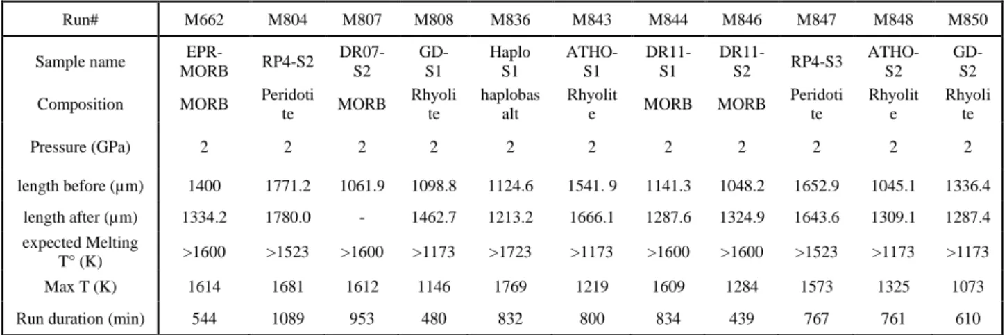
Experimental measurements of thermal diffusivities and their further transformation into 269
thermal conductivities generate uncertainties originating from the estimations of pressure, 270
temperature, sample dimensions and the data fitting itself. Experimental uncertainties on pressure and 271
temperature are presented above (~0.1 GPa and ~5 K, respectively). Sample lengths prior to the 272
sample loading (d0) and after the melting experiments were determined with a high precision digital
273
gauge (accuracy of ~1 µm) and using the Scanning Electron Microscope (FEG-SEM), respectively 274
(see Table 1). Then, the sample radius during the experiment at high pressure and temperature was 275 calculated using: 276 𝑑(𝑃, 𝑇) = 𝑑0∗ (1 − 𝛼(𝑇 − 298) + 𝑃 𝐾) −1 3⁄ (14) 277
where α is the thermal expansion and K the bulk modulus of the sample. For these calculations only 278
samples radii before experiments were considered, as post mortem measurements are affected by 279
decompression cracks (highlighted by the larger values measured after the experiments in Table 1). 280
Moreover, the distance between the two thermocouples could not be measured precisely for a few 281
samples. The values of all experimental parameters are provided in Supplementary Materials (Text 282
S4 and Figure S4). Altogether, final uncertainty on the sample length is between 5 and 10 µm. 283
There are other uncertainties associated with the procedure of data fitting for the determination 284
of raw thermal diffusivities. Experimental phase shifts and amplitude ratios (Eqs. 9 and 10) are 285
determined with a precision generally better than 1% and majored by 3% in the worst cases. In the 286
course of the Monte Carlo simulation, the differences between experimental and theoretical 287
diffusivities are recorded and used a posteriori to refine uncertainties within 1 errors. 288
Then, real thermal diffusivities are refined from the raw-diffusivities using either (i) the 289
asymptotic non-linear fit for experiments presenting a dependence in frequency (Eq. 13, which yields 290
7 important uncertainties on the refined parameters) or by averaging (see Methods). The error on 291 average (𝜎𝐴𝑉𝐺) is: 292 𝜎𝐴𝑉𝐺 = √( 1 𝑛) 2 ∗ ∑ 𝜎𝐷2 1:𝑛 (15) 293
where n is the number of diffusivity measurements performed at different frequencies and D is the 294
error on each diffusivity. Raw diffusivities recovered from Monte Carlo processing have errors of 295
~1%, similar to those of phase shift and amplitude ratio. If the fitting step is realized with Eq. 13, 296
errors of raw data are used as weights in the inversion. The standard deviations are usually between 297
1 and 10% of the real asymptotic diffusivity. If the averaging method is selected, the standard 298
deviation, estimated via Eq. 15, is usually about 1% of the final value. 299
A final source of uncertainties come from other technical issues and apparatus reproducibility, 300
which are inherent to such challenging experiments. We considered that final error must be majored 301
by 5 % of the value. The relative uncertainties become even higher after conversion into thermal 302
conductivities due to uncertainties and simplifications on the sample density and heat capacity at high 303
pressure and temperature (see Supplementary Text S4). 304
305
Experimental procedure: 306
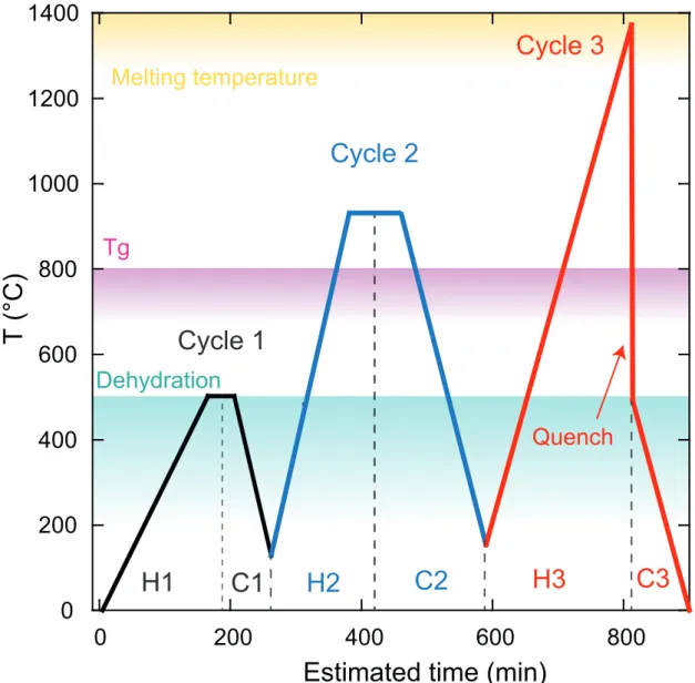
We performed a suite of three heating and cooling cycles to provide an important number of data 307
and maximize the quality of recovered data. A first cycle was run up to 500 °C for moisture removal 308
by 50°C steps (Figure. 2). The second cycle was run up to glass transition temperature (Tg) by 100°C 309
steps. Tg varies according to rock composition and its water content (Giordano et al., 2005). For our 310
dry samples, the temperature of 800°C happened to be above Tg for all our compositions. The 311
temperature was then decreased down to 150°C by 100°C steps. The quality of the measurement is 312
usually better during the cooling cycle once (1) the sample has thermally equilibrated with the 313
assembly, (2) moisture has been removed, and (3) a better contact was achieved between the sample 314
and the thermocouples due to local flow in the solid-state. The redistribution of matter under high 315
temperature cancels most of the potential artifacts associated with the presence of pores/voids 316
between the sample and the thermocouples (Hofmeister et al. 2009). Hence, data recorded during the 317
last cycles were considered for final values. 318
In the last cycle, we heated the sample up to its melting temperature by 100°C steps or 50°C near 319
the melting point. The sample was maintained above its melting point for less than 1 hour, to avoid 320
sample leakage and chemical reaction with the surrounding parts. The sample was then quenched to 321
600-550°C. This step produces a glassy sample from which measurements at low temperature are 322
performed. 323
Temperature oscillations of the two thermocouples were measured at each temperature step for 324
both heating and cooling cycles, at 12 different oscillating frequencies between 0.1 and 1.5 Hz. The 325
measurements were performed after at least 2 min of thermal equilibration to reach a stable regime 326
(the smaller is the frequency, the longer is the required equilibration time). Then, the recording 327
duration was 1 to 2 minutes or at least 10 oscillating periods. The measurement at the 12 frequencies 328
took between 20 to 30 minutes. Thus, the duration of each experiment was more than 12 hours. 329
330
Chemical and textural analyses: 331
Recovered samples were cut parallel and perpendicular to the cylindrical furnace and each 332
section was polished with great care. We could observe the position of the two thermocouples 333
junctions, measure the sample radius and perform the textural and chemical analyses (see 334
Supplementary Figures S6, S7, and S8). 335
Micro-textures were observed with a Scanning Electron Microscope (SEM) JEOL Jeol JSM-336
5910 LV using an accelerating voltage of 15 kV and a working distance of 11.4 mm. The 2D phase 337
proportions of our partially molten peridotite samples were obtained from the analyses of qualitative 338
8 chemical maps obtained by energy-dispersive X-ray spectroscopy (EDX) in the SEM. The images 339
were binarized and phases were individually separated allowing textural analyses with the FOAMS 340
software (Shea et al., 2010). A more detailed description is given in Freitas et al. (2019). On the other 341
hand, quantitative chemical analyses were performed on both our starting materials and experiment 342
products using the electron probe micro analyzer (EPMA). Chemical and textural analyses of starting 343
materials are reported in the Supplementary Text S2, Figures S6 to S13 and Tables S1, S2, S3 and 344
S4. Analyses of recovered runs are detailed in Supplementary Text S3, supplementary Figures S6 to 345
S7 and Tables S1, S2, S3 and S4. 346
Water contents were estimated using the ICP-AES for the peridotite starting materials and via 347
Raman spectroscopy for the recovered samples. Raman spectra were collected with a Renishaw InVia 348
confocal Raman micro spectrometer, equipped with a 532 nm diode laser and a Leica DM 2500M 349
optical microscope. Measurements were carried out using a 2400 grooves/mm grating, a 100×
350
microscope objective, a slit aperture set to either 20 µm or 65 µm and a laser power of 8 mW for 351
glasses and 16 or 75 mW for olivine. The resulting lateral and axial resolutions were of ~1 and 3 μm, 352
respectively, and the spectral resolution was better than 1 cm−1. Daily calibration of the spectrometer 353
was performed based on the 520.5 cm−1 peak of Si. Spectra were recorded from ~100 to 1300 cm−1 354
(alumino-silicate network domain) and from ~3000 to 3800 cm−1 (water domain), with variable 355
acquisition times ranging between 5 and 120 s for silicate bands and 120 and 240 s for water domain 356
depending on the water content (Figures S11 to S17). For water quantification in olivine and glass, 357
we followed the procedures reported by Bolfan-Casanova et al. (2014) and Schiavi et al. (2018). We 358
used both (1) the external calibration procedure, which is based on a set of hydrous olivine standards 359
from (Bolfan-Casanova et al. 2014) and different types of silicate glasses ranging from basaltic to 360
rhyolitic compositions (Schiavi et al., 2018; Médard and Grove, 2008), and (2) the internal calibration 361
procedure, based on the correlation between the water concentration in olivine or glass and the relative 362
areas of the water and silicate Raman bands (OH/Si integrated intensity ratio). The discrepancy 363
between the two methods is small. Water contents in the standard materials were previously 364
determined using the FTIR technique. 365
366
Results
367 368
We performed a total of 11 thermal diffusivity experiments on various chemical compositions, 369
using the Angström method (details in Table 1). In this section, we first describe phase shifts and 370
amplitude ratios between the two thermocouples and their conversion into thermal diffusivities and 371
conductivities. We detail the post-mortem chemical and textural analyses in the Supplementary Text 372
S3, Tables S1 to S4 and Figures S6 to S13. 373
374
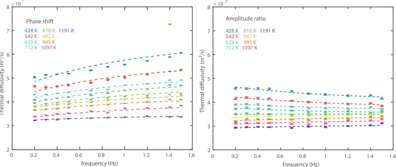
Phase shift, amplitude ratio and the refined raw-thermal diffusivities 375
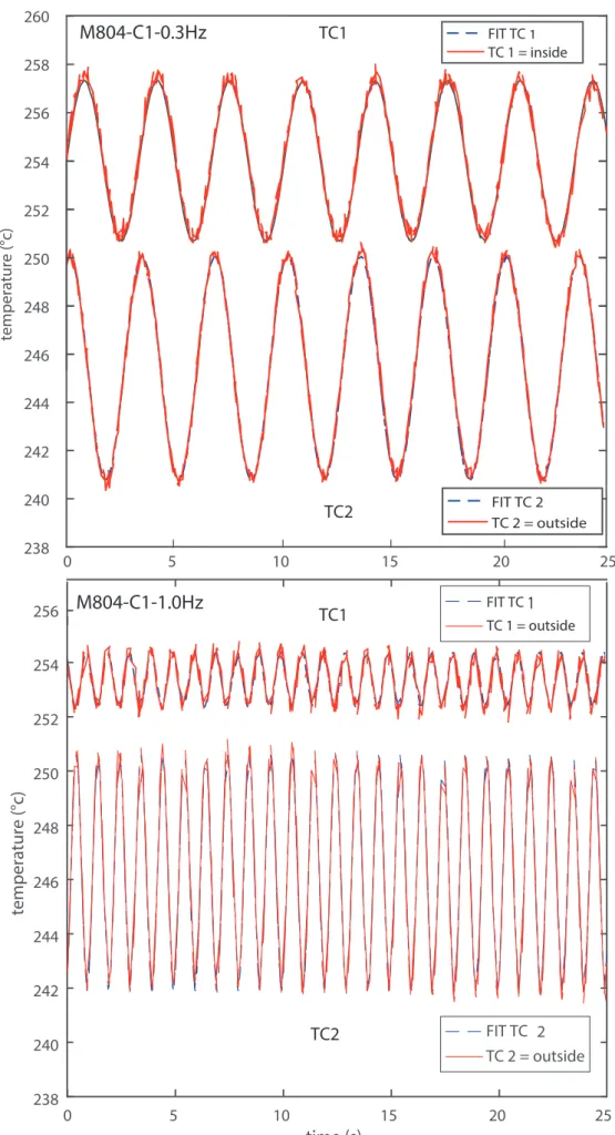
Signals recorded during the experiments are sinusoidal oscillations with varying frequencies. The 376
thermocouple located at the sample center (labeled TC1 in Figure 3) presents a phase delay and a 377
smaller amplitude compared to the thermocouple located at the sample edge (labeled TC2 in Figure 378
3). Typical raw signals and their fits are presented in Figure 3, while the refined (absolute) phase 379
shifts and amplitude ratio are reported in Figure 4. Both the magnitude of phase shift and amplitude 380
ratio change significantly with the type of sample and the experimental conditions, including the 381
source frequency. At a constant frequency, the phase shift increases with increasing temperature. At 382
a constant temperature, the phase shift increases with increasing the excitation frequency. The 383
amplitude ratio is decreasing with increasing frequency and temperature. 384
Globally, the refined thermal diffusivities present a comparable evolution of temperature at all 385
signal frequencies (see an example in Figure 5). When the frequency dependence is larger than the 386
experimental uncertainty (Figure 6), we use Eq. 13 to refine the true asymptotic value of the thermal 387
conductivity. Alternatively, when the temperature dependence is below the experimental uncertainty 388
9 or when no clear frequency trends is visible, we average the different raw-diffusivity values (see 389
Methods). In the wide majority of the cases, diffusivity values inferred from phase shifts appear to be 390
more robust and with a lesser degree of uncertainty, compared to values inferred from difference of 391
amplitude, in agreement with previous studies (Kanamori et al. 1969 and Xu et al. 2004). Hence, 392
despite similar values obtained with the two methods, values refined from phase shift were preferred. 393
394
Results for peridotite
395
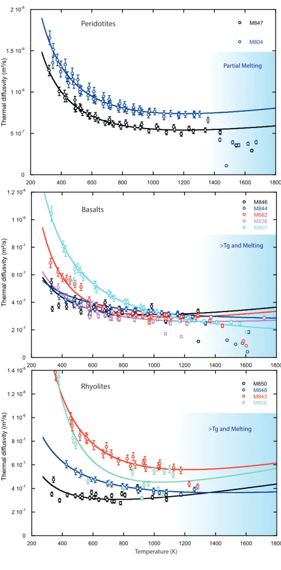
For peridotite, our two successful experiments present a smooth evolution with temperature, 396
yielding diffusivities values decreasing from 1.7(±0.1)e-6 to 7.5(±0.4)e-7 m²/s for sample M804 and 397
1.5(±0.8)e-6 to 5.5e-7 m²/s for sample M847 (Figure 6a), with an uncertainty of about 5 to 10% for 398
each sample. We attribute the relative discrepancy to a difference of sample mineralogy between the 399
two samples, due to the coarse grain size of the core drilled peridotite (see Supplementary Texts S2 400
and S3 and Figures S8 and S9). Olivine has a higher intrinsic thermal diffusivity than the other phases 401
present in peridotite such as pyroxenes and spinel (Hofmeister and Branlund, 2015). M804 may 402
contain more olivine, inducing higher diffusivities than M847. In this respect, the results for two 403
samples are thus compatible with each other and the differences are representative of the variability 404
of thermal diffusivity that can be expected among the compositional variability of peridotites (from 405
lherzolites to dunites). 406
Thermal diffusivities of our peridotite samples scale as a function of ~1/T, as expected from the 407
standard equation provided by Hofmeister and Branlund, 2015: 408
𝐷𝑙𝑎𝑡= 𝑎 ∗ 𝑇−𝑏+ 𝑐 ∗ 𝑇 (16) 409
where T is the temperature (K), and a, b and c are adjustable parameters (Table 2). The quality of the 410
fit is excellent up to a temperature of ~1300 K corresponding to the onset of peridotite melting. We 411
therefore exclude the data points above 1300 K to model the thermal properties of solid peridotite. 412
413
Results for basalts
414
For our basaltic samples, the measured diffusivities plot over a broad range of values, from 415
1.0(±0.1)e-6 to 3.0(±0.2)e-7 m²/s (Figure 6b), with an uncertainty of ~5% for each experiment. The 416
discrepancy is particularly important at low temperatures. Also, a same sample yields thermal 417
diffusivity values significantly different along the different cycles of the experimental procedure 418
(between C2, H3 and the final quench, see Figure S5). Samples with the highest diffusivities at low 419
temperatures present a rapid decrease of diffusivity with increasing temperature. On the other hand, 420
samples with the lowest diffusivities show very small temperature dependence. It yields to a 421
convergence of all diffusivity measurements at ~1000 K. Based on a study of rhyolitic glasses, 422
Romine et al. (2012) reported a moderate temperature dependence, similar to our samples presenting 423
a low diffusivity, and an increase of 0.0192 mm²/s of the glass diffusivity per percent of crystallinity. 424
For our starting materials with less than 5 vol.% of crystals (see Supplementary Text S2 and S3, 425
Figure S7), the effect of microlites could account for ~0.1 mm²/s of variation in our diffusivity values, 426
which correspond to less than ~10% of observed differences. However, the presence of 35 vol.% of 427
crystals in the recovered sample M807 would explain not only its high thermal diffusivity at low 428
temperature, but also its strong temperature dependence that is typical of crystals (see Beck et al., 429
1978; Romine et al. 2012; Hofmeister and Branlund 2015 and our peridotite trends in Figure 6a). The 430
recrystallization of M807 is not surprising, since the second cycle of annealing was performed above 431
its Tg (Figures 2 and S5). The crystallinity of other samples depends on the applied cycles of 432
annealing at a temperature eventually close to their Tg. Nonetheless, diffusivities of all samples 433
converge at increasing temperatures, because the conductivity of crystals is not much greater than 434
that of the glass at high temperature, especially if microlites are low diffusivity silicates such as 435
pyroxenes, plagioclase or spinels (see Hofmeister and Branlund 2015 for mineral diffusivity 436
compilations). Over the 5 basaltic samples investigated in this study, the diffusivity trends indicate 437
either significant recrystallization of M807 (DR07-MORB) and M662 (EPR-MORB), or negligible 438
10 crystallization of M844 and M846 (DR11-MORB) and M836 (synthetic haplobasalt). The sample 439
crystallization is likely to evolve during the thermal diffusivity measurements in step H3 (up to 440
melting point) of the experiments performed at a temperature significantly above the Tg. For this 441
reason, the crystallinity determined on the recovered samples is only a qualitative measurement of 442
the sample properties at high temperatures. 443
444
Results for rhyolites
445
Measured diffusivities of rhyolite samples also plot over a broad range of values from 1.4(±0.8)e -446
6 to 4.0(±0.2)e-7 m²/s, with an uncertainty of about 5% for each experiment (Figure 6c). The 447
discrepancy appears similar than for the basalt samples, as the sample presenting higher diffusivities 448
also show a major temperature dependence at low temperature. The presence of less than 2 vol.% of 449
crystals in the starting material could account for a diffusivity increase of 0.038 mm²/s at maximum 450
(Romine et al., 2012). Still, the diffusivity trends suggest a major recrystallization at high-temperature 451
for M808 (Güney Dag) and M843 (ATHO), some crystallization for M843 (ATHO), and negligible 452
crystallization for M850 (Güney Dag). 453
454
Properties of melts and partially molten samples
455
In addition to the evolutions described above, a strong decrease of the thermal diffusivity is 456
observed for most of our samples at the highest temperatures (Figure 6). The decrease occurs at 457
temperatures around 1300 K for peridotites, 1200 K for basalts and >1050 K for rhyolites. Such 458
temperatures are in agreement with the melting or glass transition temperatures, depending if the 459
sample is a peridotite or a glass, recrystallized or not. Similar changes were already reported at 460
temperatures above the glass transition (Hofmeister 2009, 2014, Romine et al. 2012). 461
The amplitude of the decrease is 45-50% in peridotites, which recovered samples present a degree 462
of partial melting (F) up to 23%, 35-70% for basalts and <30% for rhyolites samples. The more 463
pronounced decrease in molten peridotites is probably due to a more contrasted change of the local 464
structure at the melting point, between the minerals and the melt (see discussion). On the other hand, 465
the minor change of diffusivity for rhyolites at Tg could be related to their high SiO2-content, which 466
preserves a polymerized structure in the melt above the glass transition. 467
468
Thermal conductivities 469
Thermal conductivities (𝜅) can then be computed from thermal diffusivities following: 470
𝜅 (𝑃, 𝑇) = 𝐷(𝑃, 𝑇) ∗ 𝜌(𝑃, 𝑇) ∗ 𝐶𝑃(𝑃, 𝑇) (17) 471
where 𝜌(𝑃, 𝑇) and 𝐶𝑃(𝑃, 𝑇)are the sample density and heat capacity, respectively. For our calculations, 472
we considered and Cp values in standard conditions when the P and/or T dependences were not 473
available in the literature (see Supplementary Text S4 and Figure S4). 474
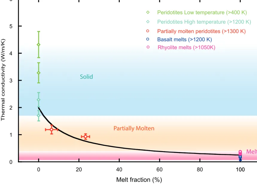
Conductivities calculated for peridotites evolve from 4.32 (±0.48) to 1.70 (±0.19) W/m/K with 475
increasing the temperature up to the melting point. Values for basalts range from 1.7 (±8.0e-2) to 0.5 476
(±4.0e-2) W/m/K, whereas those for rhyolite lie between 1.1 (±9.0e-2) and 0.3 (±3.0e-2) W/m/K for 477
low to high temperatures, respectively. At the melting temperature, our partially molten peridotites 478
display values of 1.19 (±0.16) to 0.93 (±0.10) W/m/K, whereas melts present relatively lower values 479
of 0.34 (±0.2) to 0.18 (±0.1) W/m/K for basaltic and 0.41 (±0.3) to 0.31 (±0.3) for rhyolitic 480
compositions (See Figure 7 and Table 3). We note that the important difference in conductivity 481
between basalts and rhyolites (Figure 7) is predominantly due to differences between their heat 482
capacities and densities, while their thermal diffusivities are found similar (Figure 6). 483
484
Interpretation of results
485 486
General Temperature dependence 487
11 For all compositions investigated in this study, thermal diffusivities decrease with increasing 488
temperature until reaching a plateau at temperatures between 700 and 1000 K. Based on experiments 489
performed at room pressure, it was observed that the plateau occurs at about the Debye temperature 490
of the mantle minerals (Hofmeister et al. 2009, 2014). For this reason, it was proposed that thermal 491
diffusivities vary largely with temperature until the complete activation of the vibration modes 492
(phonons in minerals). The temperature range observed in our study for the occurrence of a plateau 493
is fully compatible with this interpretation. 494
For basaltic glasses, a comparable but more moderate decrease of thermal diffusivity was 495
reported up to a saturation temperature corresponding well to the glass Tg (Hofmeister et al. 2009, 496
2014, Romine et al. 2012). In our experiments, the decrease is of ~30% to 60% over the investigated 497
temperature range, depending on the experiment. Such amplitude is compatible with the ~40% 498
decrease observed during the heating of pyroxene glasses (Hofmeister et al. 2009). 499
For rhyolite samples, the thermal conductivity increases slightly with increasing the temperature 500
(Figure 7). This is due to the heat capacity that increases more with temperature than the density 501
increases and diffusivity decreases (Eq. 17). The increase is, however, smaller than reported in 502
Romine et al. (2012), due to the use of a different Cp (Neuville et al. 1993) (see Supplementary Text 503
S4) and a stronger temperature dependence of thermal diffusivities observed in our experiments 504
because of different crystallizations states. 505
506
Effect of radiative conduction 507
Romine et al. (2012) reported an increase in thermal diffusivities of the melts at very high 508
temperatures at ambient pressure. They attributed this feature to an increased role of the radiative 509
component. Such a component can dominate the thermal diffusivity for a sample transparent to the 510
infrared and visible photons at high temperatures. For thin samples, this effect can become 511
problematic if the mean free path of photons is longer than the sample length (ballistic photons, see 512
Hofmeister and Branlund, 2015). No significant increase in thermal diffusivity and conductivity is 513
observed in our high-pressure experiments, except maybe for the rhyolitic samples (Figures 6 and 7). 514
The difference with the previous work is most probably related to the opacity of our basalts and 515
peridotites samples, hence limiting the radiative transfers. 516
517
Effect of glass/melt composition 518
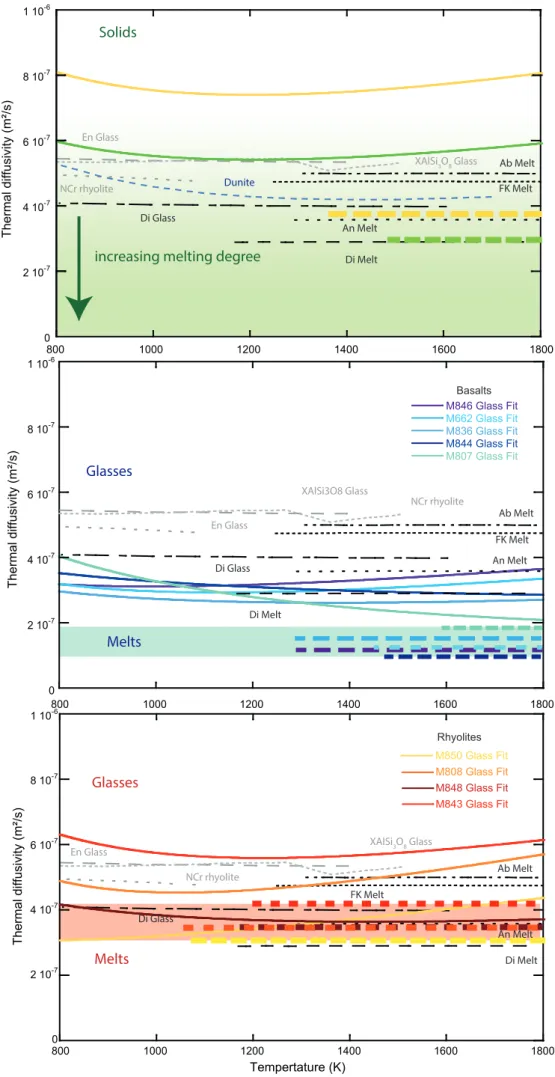
Overall, our conductivity values are compatible with the values available in the literature (see 519
Figure 8). Differences in absolute values are nonetheless present. Rhyolite melts (0.31-0.41 W/m/K) 520
are found slightly more conductive than basaltic ones (0.18-0.34 W/m/K). Within the same family of 521
glass, thermal conductivity varies by 0.10 to 0.15 W/m/K for rhyolitic and basaltic melts, respectively. 522
This is slightly larger (of at least 10%) than the experimental uncertainty, an effect possibly due to 523
larger uncertainties on the dimensions of the molten sample. No clear trend can be retrieved from the 524
comparison between our different basaltic or rhyolitic compositions. Among the major elements, iron 525
could be of major importance, due to its critical impact on glass/melt density. Indeed, the thermal 526
diffusivity of glasses was reported to decrease with increasing density (Hofmeister 2014). The 527
comparison between our rhyolites and basalts is coherent with such a trend. However, our haplobasalt 528
(M836) presents diffusivity values comparable with natural basalts (M662, M807, M844), as well as 529
Fe-bearing (M843 and M848) and Fe-free (M808 and M850) rhyolites (Figure 6), despite a variation 530
of the Fe-content from 0 to 10 wt.% in these different samples. Other elements could also impact the 531
melt thermal diffusivity, in particular Si and Al, which favor polymerization of the liquid (and alkali 532
elements for the opposite effect) (Ni et al. 2015). Still, within the experimental uncertainty, we 533
observe no clear trend related to these elements, despite a variation of the SiO2 content by more than 534
20%. Additionally, water, with a total content smaller than 1.10 wt.%, should have a negligible effect 535
on thermal conductivity (Romine et al. 2012, Ni et al. 2015). It could, however, impact the melt 536
density at a low degree of partial melting (Hofmeister 2014). As the water contents estimated in the 537
12 recovered samples are similar to the ones obtained in starting materials (see Supplementary Text S2 538
and S3), water should not induce any strong diffusivity variation in our data-set. We, therefore, 539
conclude that chemical effects are secondary compared to the structural ones. 540
541
Mixing models for thermal conductivities of partially molten peridotite 542
Our results show that peridotites, and to a lower extent the glasses, present higher thermal 543
diffusivities compared to the melts. This result is not surprising: thermal conductivity is strongly 544
dependent on the local structure and its vibrational properties. The disorder in the atomic structure 545
increases from solid, glasses to molten states (Hofmeister et al. 2014). The composition of the melt 546
appears to be of secondary importance. The final set of thermal diffusivities and conductivities values 547
selected for the applications are given in Tables 3, S5 and Figures 9 and S14. 548
To propose a predictive law for thermal conductivity of partially molten rocks several mixing 549
equations are now tested. Such equation generally describes the effect of a small amount of 550
conductive phase into an insulating matrix. For thermal conduction, the problem is reversed because 551
the melt is less conductive than the solid. In this section, we explore the different predictive models 552
of thermal conductivity of binary mixtures: 553
1) Linear mixing model consider parallel thermal resistor: 554
𝜅𝑏𝑢𝑙𝑘= 𝜅𝑠∗ (1 − 𝐹) + 𝐹𝜅𝑚(18) 555
Where s corresponds to the solid, m the melt and F the volume fraction of the melt. 556
2) tube / Ashbie model consider 1/3 of tubes of melt aligned in the heat flow direction (Grant and 557 West, 1965, Schmeling 1986): 558 𝜅𝑏𝑢𝑙𝑘= 1 3∗ 𝜅𝑠∗ (1 − 𝐹) + 𝐹𝜅𝑚 (19) 559
3) cube model (Waff, 1974) representing cubes of solids into a melt matrix 560
𝜅𝑏𝑢𝑙𝑘= [1 − 𝐹2/3] ∗ 𝜅𝑠 (20) 561
4) Archie’s law, an empirical relation developed for electrical conductivity (Watanabe and Kurita, 562
1983) 563
𝜅𝑏𝑢𝑙𝑘= 𝐶 ∗ (1 − 𝐹)𝑛∗ 𝜅𝑠(21) 564
Where C and n are constants. 565
5) Thermal resistors in series: 566 𝜅𝑏𝑢𝑙𝑘= 𝜅𝑠∗ 𝜅𝑚⁄𝜅𝑠 𝜅𝑚⁄𝜅𝑠+ 𝐹(1 − 𝜅𝑚⁄𝜅𝑠) (22) 567
6) Hashin Shtrikman lower bound (HS-), representing insulating melt spheres into a conductive solid 568 matrix: 569 𝜅𝑏𝑢𝑙𝑘= 𝜅𝑠∗ 𝐹 1/(𝜅𝑚⁄𝜅𝑠)+1 − 𝐹3𝜅 𝑠 (23) 570 7) Maxwell-Eucken relation: 571 𝜅𝑏𝑢𝑙𝑘= 𝜅𝑠∗ 𝜅𝑚+ 2𝜅𝑠+ 2𝐹(𝜅𝑚− 𝜅𝑠) 𝜅𝑚+ 2𝜅𝑠− 𝐹(𝜅𝑚− 𝜅𝑠) (24) 572 573
8) Landauer relation, based on resistors in series: 574 𝜅𝑏𝑢𝑙𝑘= 1 4∗ [𝜅𝑚(3𝐹 − 1) + 𝜅𝑠(2 − 3𝐹) + {(𝜅𝑚(3𝐹 − 1) + 𝜅𝑠(2 − 3𝐹))² + 8𝜅𝑠𝜅𝑚} 1 2] (25) 575 576 9) Russel-Rayleigh relation: 577 𝜅𝑏𝑢𝑙𝑘= 𝜅𝑠[𝜅𝑠+𝐹2/3(𝜅𝑚−𝜅𝑠)] 𝜅𝑠+ (𝜅𝑚− 𝜅𝑠)(𝜅𝑚 2 3− 𝐹) (26) 578 579
13 These equations provide a different evolution of the thermal conductivity with the fraction of melt 580
(F). In Figure S14, we present the results when either fixing 𝜅solid and 𝜅melt to the average value of our 581
measurements, or adjusting their values to minimize the misfit between the mixing models and our 582
results at varying F values (Table S5). Among the variety of fits obtained, it appears that the effect of 583
partial melting is underestimated in most of the cases. Only the thermal resistors in series is capable 584
to reproduce adequately the strong curvature observed experimentally at low F values, as well as the 585
end-member values of solid and melt conductivities. For this reason, we use series model (eq. 22) for 586
further discussions. 587
We note a lack of data points at high melt fractions, preventing to decipher more precisely the 588
mixing trend. At very high temperatures, the experimental measurements become difficult on natural 589
peridotite melting, in particular due to melt escape and chemical reactions with the experimental cell. 590
Complementary data could be acquired working with analog system such as basalt/olivine mixture 591
and could represent a further research direction. 592
593
Thermal conductivity of partially molten peridotite: influence of texture 594
The 3D solid/melt arrangement is known to influence significantly the geophysical properties 595
of partially molten systems (von Bargen and Waff, 1986; Laporte et al., 1997; Laporte and Provost, 596
2000, Minarik and Watson, 1995; Yoshino et al., 2005 Maumus et al. 2005; Ten Grotenhuis et al. 597
2005, Freitas et al. 2019). Their distribution is classically described using dihedral angle value, which 598
translates the ability of a liquid to wet the grain boundaries as a consequence of interfacial energies. 599
The dihedral angle decreases when increasing pressure, temperature, water content and decreasing 600
silica/alumina content of the melt (Yoshino et al. 2007, Mibe et al. 1998, 1999, Laporte et al., 1997, 601
Watson et al 1991). Several studies with similar basaltic or peridotite melts (dry) have shown that 602
basalt-like melts at mantle conditions have dihedral angles significantly lower than the 603
interconnection threshold of 60°, with values between 30-40° at 2 GPa (Laporte et al., 1997, Yoshino 604
et al. 2005, 2007). Our partially molten samples display a coherent texture and dihedral angles with 605
these observations. Dihedral angles of 23.3° and 19.0° were measured from our samples containing 606
6.4% and 23.3% of melt, respectively (Figure S15), in good agreement with previous data given that 607
these mafic melts are moderately hydrous (Table S3). For each melt fraction, a thin layer of melt 608
surround most of the grains, in particular olivines, which in 3D will result into the insulation of the 609
solid gains from their surroundings (Figure S9). This is very well visible on our low melt fraction 610
sample (F=6.4%) where the layers of melt are few microns thick (M804). Even if melt is more 611
abundant near clinopyroxenes and spinel sites in M847 (F=23.3%), the melt pockets are 612
interconnected with similar thin melt layers (<10 µm) (Figure S9). As a result, thermal conductivity 613
is expected to drop brutally in the first degrees of melting. Still, some grain boundaries should remain 614
un-wetted until the melt fraction rise significantly. For this reason, thermal conductivity should only 615
stabilize at melt fraction corresponding to solid grains completely isolated from each other. This trend 616
is visible in our data and parallel model (Figures 9 and S14) with a strong decrease in the first 10% 617
of melting highlighted by M804, the change of slope seems to occur around 15% and values decease 618
more slowly in the 15-50% range as seen in M847, to stabilize and display near-melt values above 619
50%. The complete isolation of solids should occur at “packing” threshold, which is a function of the 620
solid shapes and size distribution and is expected to occur between 40 to 60% of melting. Thus, the 621
first degrees of melting are very crucial in the case of a wetting liquid and affecting importantly the 622
thermal properties. 623
624
Thermal conductivity of peridotite: effect of the grain size 625
The modelling of thermal conductivity of peridotites and low F molten peridotites should also 626
take in account the effect of grain boundaries thermal resistances as grain size may vary in the 627
different geological contexts (from 100 µm to >1 cm), as seen in natural meteoritic examples, (Barrat 628
et al. 1999, Busek, 1977, Keil, 2010, Floran et al. 1978). Indeed, grain boundary scattering could be 629
14 important when the mean free paths of phonons approach the grain size. This effect, which only 630
concerns solids and low fractions of melt, can be quantified with the following equation (Smith et al. 631 2003, Smith et al. 2013): 632 1 𝜅𝑝𝑜𝑙𝑦 = 1 𝜅𝑠𝑖𝑛𝑔𝑙𝑒 + 𝑛𝑅𝑏𝑜𝑢𝑛𝑑𝑎𝑟𝑦(27) 633
Where 𝜅𝑝𝑜𝑙𝑦 is the thermal conductivity of the polycrystalline sample, 𝜅𝑠𝑖𝑛𝑔𝑙𝑒 the thermal 634
conductivity of a reference single crystal (average from olivine data of Hofmeister et al. 2016, Table 635
3), n represents the surface of grain boundaries along the heat flow direction per unit length, and 636
Rboundary the thermal resistance of grain boundary plane. The n value should be almost constant with
637
temperature (Smith et al. 2013) and is estimated between 4e-4 and 7e-3 m for our two peridotite 638
samples via analyses of SEM images (grain size ranging from 25 to 140 µm, see Table S4 for textural 639
parameters). We calculate Rboundary values between 1.9e-6 and 5.9e-6 W/m²/K for M804 and 9.3e-6 and
640
3.2e-5 W/m²/K for M847. These values are compatible or slightly higher than hydrous polycrystalline 641
olivine samples (Zhang et al. 2019). 642
As a result, the thermal conductivities quantified in our experiments are underestimations of 643
natural ones as the grain size is <100 µm, in experiments compared to grain sizes of 100 µm up to >1 644
cm typical of mantle peridotites and reduced meteorites (which could be relic of bodies interiors, 645
from cumulates (Floran et al. 1978), enstatite chondrite/achondrite (Keil, 2010), diogenite (Barrat et 646
al. 1999) to pallasite (Busek, 1977)). Melts and high F partially molten systems are not affected by 647
such effect, thus the observed decrease of thermal conductivity at the melting temperature is probably 648
smaller in our experiments. 649
650
Implications for geodynamos on Mercury-like proto-planets
651 652
Suitable conditions for a dynamo 653
For a thermally driven dynamo to operate in a terrestrial planet, four conditions were found to be 654
necessary (e.g., Monteux et al., 2011): the core heat flow must be at least adiabatic (1), the thermal 655
convection within the core has to supply enough power to compensate the losses due to ohmic 656
dissipation (2), the Reynolds magnetic number must be supercritical (complex turbulent convection) 657
(3) and the mantle heat flow has to overcome the core heat flow needed to induce a dynamo (4). These 658
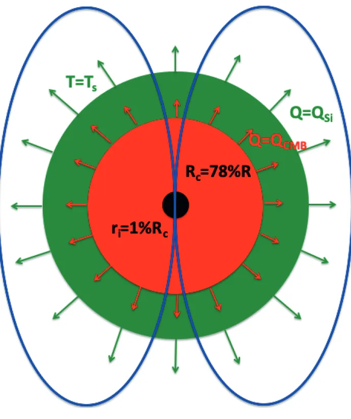
conditions can be expressed in terms of heat flow balance (See Figure 10 for a schematic 659
representation) and are detailed here: 660
661
(1) The metallic core has to convect, meaning that the heat flow out of the core needs to overcome
662
the adiabatic heat flow (Stevenson et al., 1983).
663
For this, the core thermal conductivity (𝜅core) is a dominant parameter. A large 𝜅core value 664
increases the heat flux along the core adiabat and reduces the lifetime of a thermally driven dynamo 665
(Breuer et al., 2015). Several laboratory measurements suggested that the thermal conductivity of 666
polycrystalline iron at Mercury's core conditions is 113–125 W/m/K (see Deng et al., 2013 and 667
references therein). However, such values for Mercury are recently challenged with several recent 668
studies proposing a much lower conductivity. In a first one, the conductivity of pure Fe and Fe-Si 669
alloys is reported at 30-40 W/m/K and 35-40 W/m/K, respectively (Sibert et al. 2019). Then, it is 670
proposed that the thermal conductivity of Fe‐S at the P-T conditions of Mercury's core is as low as 671
~4 W/m/K, thus 1-2 orders of magnitude lower than that of pure iron (Pommier et al. 2019, 672
Manthilake et al. 2019). 673
This first condition can be expressed as: 674 675 𝑄𝐶𝑀𝐵> 𝑄𝐴𝑑= 𝜅𝑐𝛼𝑐𝑔𝑐𝑇𝐶𝑀𝐵 𝐶𝑝,𝑐 4𝜋𝑅𝑐2 (28) 676
15 To estimate this flux, we assume that TCMB is the melting temperature of pure iron at PCMB. This 677
assumption gives a conservative value of the core heat flow in comparison with considering TICB 678
since the core liquidus is steeper that the core adiabat. We estimate the relation between the melting 679
temperature of pure iron and the pressure using the following expression obtained by fitting the 680
experimental results from Anzellini et al. 2013 with a Simon and Glatzel equation: 681 𝑇𝑚,𝐹𝑒 = 1800 ( 𝑃𝐶𝑀𝐵 27.9 + 1) 1/2.08 (29) 682
Such a melting temperature typically lies between the solidus and liquidus of a chondritic mantle 683
for the same pressure conditions (Monteux et al. 2020 and references therein). We also assume that 684
𝑘𝑐, 𝛼𝑐 and 𝐶𝑝,𝑐 are constant (see values in Table 4) and 𝑃𝐶𝑀𝐵 is calculated as follows (Monteux and 685 Arkani-Hamed, 2014): 686 𝑃𝐶𝑀𝐵= 𝑃(𝑟 = 𝑅𝑐) = 2 3𝜋𝐺𝜌𝑐 2(𝑅 𝑐2− 𝑟2) + 2 3𝜋𝐺𝜌𝑆𝑖 2(𝑅2− 𝑅 𝑐2) + 4 3𝜋𝐺𝜌𝑆𝑖𝑅𝑐 3(𝜌 𝑐− 𝜌𝑆𝑖) ( 1 𝑅𝑐 −1 𝑅) (30) 687 688
(2) The energy supplied by thermal convection to the geodynamo has to compensate for the loss due
689
to ohmic decay (Buffett, 2002).
690
This imposes a condition on the core heat flow at the CMB. In fact, core heat flow will need to 691
overcome a critical value. Assuming that dynamo is generated only by thermal convection in the core, 692 we can write: 693 𝑄𝐶𝑀𝐵 > 𝑄𝐴𝑑+ 4𝜐𝑐𝐵̅2𝐶𝑝,𝑐 0.8𝜇𝑐𝛼𝑐𝐺𝜌𝑐𝑅𝑐 (31) 694
This heat flux is estimated by considering that the characteristic magnetic length scale equals the 695
radius of the core. The parameter 𝐵̅ is the average strength of the magnetic field inside the core and 696
was estimated using a scaling from Christensen and Aubert (2006): 697 𝐵̅ = 0.9𝜇𝑐 1 2𝜌𝑐 1 6(𝑔𝑐𝑄𝐵(𝑅𝑐− 𝑟𝑖) 4𝜋𝑅𝑐𝑟𝑖 ) 1 3 (32) 698
With 𝑄𝐵 = 𝛼𝑐𝑄𝐶𝑀𝐵/𝐶𝑝,𝑐 the buoyancy flux and ri the radius of the inner core. In the scaling from
699
Christensen and Aubert (2006), the inner core size cannot be set to 0. On Mercury the size of the 700
inner core is currently not well constrained even if recent constraints via geodetic analysis (Genova 701
et al. 2018) suggest its presence and a possible important size (ri/Rc between 0.3 and 0.7). As we focus
702
here on the effect of thermal cooling on dynamo generation (i.e. we do not consider the effect of 703
compositional convection related to inner core growth), we consider a small inner core with 𝑟𝑖/𝑅𝑐 = 704
0.01. The scaling law used to calculate the average strength of the magnetic field inside the core (Eq. 705
32) is valid for the Earth but overestimates 𝐵̅ in the case of thin shell dynamos such as the one 706
operating within Mercury (Christensen and Aubert (2006)). Mariner 10 spacecraft measurements 707
showed that Mercury’s magnetic field was 100 times weaker than the Earth’s one. To account for this 708
discrepancy, we consider that the average strength of the magnetic field is 1%𝐵̅ obtained from Eq. 32 709
when solving Eq. 31. We also consider that 𝜐𝑐, 𝜇𝑐 and 𝜌𝑐 are constants (see values in Tab. 4). We 710
note that most of the power needed to overcome the criterion related to Eq. 31 can be supplied by 711
thermal core convection (i.e. criterion related to Eq. 28) especially for large metallic cores. 712
713
(3) The magnetic Reynolds number (Rem) must be supercritical in order to have convective motions,
714
inducing a complex structure needed to carry the magnetic field lines (U. R. Christensen and Aubert,
715
2006).
716
Reynolds magnetic number is calculated using Christensen and Aubert, 2006 formulation’s and 717
assuming that the characteristic magnetic length scale is the radius of the core: 718 𝑅𝑒𝑚 = ( 𝑄𝐶𝑀𝐵𝐺𝛼𝑐 3𝐶𝑝,𝑐 ) 1/3 𝑅𝑐 𝜐𝑐 > 10 − 100 (33) 719