Adaptive Concretization for Parallel Program Synthesis
The MIT Faculty has made this article openly available.
Please share
how this access benefits you. Your story matters.
Citation
Jeon, Jinseong, et al. “Adaptive Concretization for Parallel Program
Synthesis.” Lecture Notes in Computer Science (2015): 377–394. ©
2015 Springer International Publishing Switzerland
As Published
http://dx.doi.org/10.1007/978-3-319-21668-3_22
Publisher
Springer-Verlag
Version
Author's final manuscript
Citable link
http://hdl.handle.net/1721.1/111033
Terms of Use
Creative Commons Attribution-Noncommercial-Share Alike
Adaptive Concretization for
Parallel Program Synthesis
?Jinseong Jeon1, Xiaokang Qiu2,
Armando Solar-Lezama2, and Jeffrey S. Foster1
1 University of Maryland, College Park 2
Massachusetts Institute of Technology
Abstract. Program synthesis tools work by searching for an implemen-tation that satisfies a given specification. Two popular search strategies are symbolic search, which reduces synthesis to a formula passed to a SAT solver, and explicit search, which uses brute force or random search to find a solution. In this paper, we propose adaptive concretization, a novel synthesis algorithm that combines the best of symbolic and explicit search. Our algorithm works by partially concretizing a randomly chosen, but likely highly influential, subset of the unknowns to be synthesized. Adaptive concretization uses an online search process to find the opti-mal size of the concretized subset using a combination of exponential hill climbing and binary search, employing a statistical test to determine when one degree of concretization is sufficiently better than another. Moreover, our algorithm lends itself to a highly parallel implementation, further speeding up search. We implemented adaptive concretization for Sketch and evaluated it on a range of benchmarks. We found adaptive concretization is very effective, outperforming Sketch in many cases, sometimes significantly, and has good parallel scalability.
1
Introduction
Program synthesis aims to construct a program satisfying a given specification. One popular style of program synthesis is syntax-guided synthesis, which starts with a structural hypothesis describing the shape of possible programs, and then searches through the space of candidates until it finds a solution. Recent years have seen a number of successful applications of syntax-guided synthesis, ranging from automated grading [18], to programming by example [8], to synthesis of cache coherence protocols [22], among many others [6, 14, 20].
Despite their common conceptual framework, each of these systems relies on different synthesis procedures. One key algorithmic distinction is that some use explicit search—either stochastically or systematically enumerating the candi-date program space—and others use symbolic search—encoding the search space as constraints that are solved using a SAT solver. The SyGuS competition has recently revealed that neither approach is strictly better than the other [1].
?
Supported in part by NSF CCF-1139021, CCF-1139056, CCF-1161775, and the part-nership between UMIACS and the Laboratory for Telecommunication Sciences.
In this paper, we propose adaptive concretization, a new approach to syn-thesis that combines many of the benefits of explicit and symbolic search while also parallelizing very naturally, allowing us to leverage large-scale, multi-core machines. Adaptive concretization is based on the observation that in synthe-sis via symbolic search, the unknowns that parameterize the search space are not all equally important in terms of solving time. In Section 2, we show that while symbolic methods can efficiently solve for some unknowns, others—which we call highly influential unknowns—cause synthesis time to grow dramatically. Adaptive concretization uses explicit search to concretize influential unknowns with randomly chosen values and searches symbolically for the remaining un-knowns. We have explored adaptive concretization in the context of the Sketch synthesis system [19], although we believe the technique can be readily applied to other symbolic synthesis systems such as Brahma [12] or Rosette [21].
Combining symbolic and explicit search requires solving two challenges. First, there is no practical way to compute the precise influence of an unknown. Instead, our algorithm estimates that an unknown is highly influential if concretizing it will likely shrink the constraint representation of the problem. Second, because influence computations are estimates, even the highest influence unknown may not affect the solving time for some problems. Thus, our algorithm uses a series of trials, each of which makes an independent decision of what to randomly concretize. This decision is parameterized by a degree of concretization, which adjusts the probability of concretizing a high influence unknown. At degree 1, unknowns are concretized with high probability; at degree ∞, the probability drops to zero. The degree of concretization poses its own challenge: a preliminary experiment showed that across seven benchmarks and six degrees, there is a different optimal degree for almost every benchmark. (Section 3 describes the influence calculation, the degree of concretization, and this experiment.)
Since there is no fixed optimal degree, the crux of adaptive concretization is to estimate the optimal degree online. Our algorithm begins with a very low degree (i.e., a large amount of concretization), since trials are extremely fast. It then exponentially increases the degree (i.e., reduces the amount of concretiza-tion) until removing more concretization is estimated to no longer be worthwhile. Since there is randomness across the trials, we use a statistical test to determine when a difference is meaningful. Once the exponential climb stops, our algorithm does binary search between the last two exponents to find the optimal degree, and it finishes by running with that degree. At any time during this process, the algorithm exits if it finds a solution. Adaptive concretization naturally paral-lelizes by using different cores to run the many different trials of the algorithm. Thus a key benefit of our technique is that, by exploiting parallelism on big ma-chines, it can solve otherwise intractable synthesis problems. (Section 4 discusses pseudocode for the adaptive concretization algorithm.)
We implemented our algorithm for Sketch and evaluated it against 26 benchmarks from a number of synthesis applications including automated tu-toring [18], automated query synthesis [6], and high-performance computing, as well as benchmarks from the Sketch performance benchmark suite [19] and
from the SyGuS’14 competition [1]. By running our algorithm over twelve thou-sand times across all benchmarks, we are able to present a detailed assessment of its performance characteristics. We found our algorithm outperforms Sketch on 23 of 26 benchmarks, sometimes achieving significant speedups of 3× up to 14×. In one case, adaptive concretization succeeds where Sketch runs out of memory. We also ran adaptive concretization on 1, 4, and 32 cores, and found it generally has reasonable parallel scalability. Finally, we compared adaptive concretization to the winner of the SyGuS’14 competition on a subset of the SyGuS’14 benchmarks and found that our approach is competitive with or out-performs the winner. (Section 5 presents our results in detail.)
2
Combining Symbolic and Explicit Search
To illustrate the idea of influence, consider the following Sketch example:
bit [32] foo(bit [32] x) implements spec{ if (??){
return x & ??; // unknown m1 }else{
return x | ??; // unknown m2 } }
bit [32] spec(bit [32] x){ return minus(x, mod(x, 8)); }
Here the symbol??represents an unknown constant whose type is automatically inferred. Thus, the ??in the branch condition is a boolean, and the other ??’s, labeled as unknowns m1 and m2, are 32-bit integers. The specification on the right asserts that the synthesized code must compute(x − (x mod 8)).
The sketch above has 65 unknown bits and 233unique solutions, which is too
large for a naive enumerative search. However, the problem is easy to solve with symbolic search. Symbolic search works by symbolically executing the template to generate constraints among those unknowns, and then generating a series of SAT problems that solve the unknowns for well-chosen test inputs. Using this approach, Sketch solves this problem in about 50ms, which is certainly fast.
However, not all unknowns in this problem are equal. While the bit-vector unknowns are well-suited to symbolic search, the unknown in the branch is much better suited to explicit search. In fact, if we incorrectly concretize that unknown to false, it takes only 2ms to discover the problem is unsatisfiable. If we concretize it correctly to true, it takes 30ms to find a correct answer. Thus, enumerating concrete values lets us solve the problem in 32ms (or 30ms if in parallel), which is 35% faster than pure symbolic search. For larger benchmarks this can make the difference between solving a problem in seconds and not solving it at all.
The benefit of concretization may seem counterintuitive since SAT solvers also make random guesses, using sophisticated heuristics to decide which vari-ables to guess first. To understand why explicit search for this unknown is ben-eficial, we need to first explain how Sketch solves for these unknowns. First, symbolic execution in Sketch produces a predicate of the form Q(x, c), where
x is the 32-bit input bit-vector and c is a 65-bit control bit-vector encoding the unknowns. Q(x, c) is true if and only if foo(x)=x−(x mod 8) for the function foo
described by c. Thus, Sketch’s goal is to solve the formula ∃c.∀x.Q(x, c). This is a doubly quantified problem, so it cannot be solved directly with SAT.
Sketch reduces this problem to a series of problems of the form ∧xi∈EQ(xi, c),
i.e., rather than solving for all x, Sketch solves for all xi in a carefully chosen
set E. After solving one of these problems, the candidate solution c is checked symbolically against all possible inputs. If a counterexample input is discovered, that counterexample is added to the set E and the process is repeated. This is the Counter-Example Guided Inductive Synthesis (CEGIS) algorithm, and it is used by most published synthesizers (e.g., [12, 21, 22]).
Sketch’s solver represents constraints as a graph, similar to SMT solvers, and then iteratively solves SAT problems generated from this graph. The graph is essentially an AST of the formula, where each node corresponds to an unknown or an operation in the theory of booleans, integer arithmetic, or arrays, and where common sub-trees are shared (see [19] for more details). For the simple example above, the formula Q(x, c) has 488 nodes and CEGIS takes 12 iterations. On each iteration, the algorithm concretizes xi and simplifies the formula to 195 nodes.
In contrast, when we concretize the condition, Q(x, c) shrinks from 488 to 391 nodes, which simplify to 82 nodes per CEGIS iteration. Over 12 iterations, this factor of two in the size of the problem adds up. Moreover, when we concretize the condition to the wrong value, Sketch discovers the problem is unsatisfiable after only one counterexample, which is why that case takes only 2ms to solve.
In short, unlike the random assignments the SAT solver uses for each individ-ual sub-problem in the CEGIS loop, by assigning concrete values in the high-level representation, our algorithm significantly reduces the sub-problem sizes across all CEGIS loop iterations. It is worth emphasizing that the unknown controlling the branch is special. For example, if we concretize one of the bits in m1, it only reduces the formula from 488 to 486 nodes, and the solution time does not improve. Worse, if we concretize incorrectly, it will take almost the full 50ms to discover the problem is unsatisfiable, and then we will have to flip to the correct value and take another 50ms to solve, thus doubling the solution time. Thus, it is important to concretize only the most influential unknowns.
Putting this all together yields a simple, core algorithm for concretization. Consider the original formula Q(x, c) produced by symbolic execution over the sketch. The unknown c is actually a vector of unknowns ci, each corresponding
to a different hole in the sketch. First, rank-order the ci from most to least
influence, cj0, cj1, · · ·. Then pick some threshold n smaller than the length of
c, and concretize cj0, · · · , cjn with randomly chosen values. Run the previously
described CEGIS algorithm over this partially concretized formula, and if a solution cannot be found, repeat the process with a different random assignment. Notice that this algorithm parallelizes trivially by running the same procedure on different cores, stopping when one core finds a solution.
This basic algorithm is straightforward, but three challenges remain: How to estimate the influence of an unknown, how to estimate the threshold of influence
for concretization, and how to deal with uncertainty in those estimates. We discuss these challenges in the next two sections.
3
Influence and Degree of Concretization
An ideal measure of an unknown’s influence would model its exact effect on running time, but there is no practical way to compute this. As we saw in the previous section, a reasonable alternative is to estimate how much we expect the constraint graph to shrink if we concretize a given node. However, it is still expensive to actually perform substitution and simplification.
Our solution is to use a more myopic measure of influence, focusing on the immediate neighborhood of the unknown rather than the full graph. Following the intuition from Section 2, our goal is to assign high influence to unknowns that select among alternative program fragments (e.g., used as guards of conditions), and to give low influence to unknowns in arithmetic operations. For an unknown n, we define influence(n) =P
d∈children(n)benefit(d, n), where children(n) is the
set of all nodes that depend directly on n. Here benefit(d, n) is meant to be a crude measure of how much the overall formula might shrink if we concretize the parent node n of node d. The function is defined by case analysis on d: – Choices. If d is an ite node,3, there are two possibilities. If n is d’s guard (d =
ite(n, a, b)) then benefit(d, n) = 1, since replacing a with a constant will cause the formula to shrink by at least one node. On the other hand, if n corresponds to one of the choices (d = ite(c, n, b) or d = ite(c, a, n)), then benefit(d) = 0, since replacing n with a constant has no effect on the size of the formula. – Boolean nodes. If d is any boolean node except negation, it has benefit 0.5. The intuition is that boolean nodes are often used in conditional guards, but sometimes they are not, so they have a lower benefit contribution than ite guards. If d = ¬(n), then benefit(d, n) equals influence(d), since the benefit in terms of formula size of concretizing n and d is the same.
– Choices among constants. Sketch’s constraint graph includes nodes repre-senting selection from a fixed sized array. If d corresponds to such a choice that is among an array of constants, then benefit(d, n) = influence(d), i.e., the benefit of concretizing the choice depends on how many nodes depend on d.
– Arithmetic nodes. If d is an arithmetic operation, benefit(d, n) = −∞. The intuition is that these unknowns are best left to the solver. For example, given
??+in, replacing??with a constant will not affect the size of the formula. Note that while the above definitions may involve recursive calls to influence, the recursion depth will never be more than two due to prior simplifications. This pass also eliminates nodes with no children, and thus any unknown not involved in arithmetic will have at least one child and thus an influence of at least 0.5.
Before settling on this particular influence measure, we tried a simpler ap-proach that attempted to concretize holes that flow to conditional guards, with
3
a probability based on the degree of concretization. However, we found that a small number of conditionals have a large impact on the size and complexity of the formula. Thus, having more refined heuristics to identify high influence holes is crucial to the success of the algorithm.
3.1 Degree of Concretization
The next step is to decide the threshold for concretization. We hypothesize the best amount of concretization varies—we will test this hypothesis shortly. More-over, since our influence computation is only an estimate, we opt to incorporate some randomness, so that (estimated) highly influential unknowns might not be concretized, and (estimated) non-influential unknowns might be.
Thus, we parameterize our algorithm by a degree of concretization (or just degree). For each unknown n in the constraint graph, we calculate its estimated influence N = influence(n). Then we concretize the node with probability
p = 0 if N < 0 1.0 if N > 1500 1/(max(2, degree/N )) otherwise
To understand this formula, ignore the first two cases, and consider what hap-pens when degree is low, e.g., 10. Then any node for which N ≥ 5 will have a 1/2 chance of being concretized, and even if N is just 0.5—the minimum N for an unknown not involved in arithmetic—there is still a 1/20 chance of concretiza-tion. Thus, low degree means many nodes will be concretized. In the extreme, if degree is 0 then all nodes have a 1/2 chance of concretization. On the other hand, suppose degree is high, e.g., 2000. Then a node with N = 5 has just a 1/400 chance of concretization, and only nodes with N ≥ 1000 would have a 1/2 chance. Thus, a high degree means fewer nodes will be concretized, and at the extreme of degree = ∞, no concretization will occur, just as in regular Sketch. For nodes with influence above 1500, the effect on the size of the formula is so large that we always find concretization profitable. Nodes with influence below zero are those involved in arithmetic, which we never concretize.
Overall, there are four “magic numbers” in our algorithm so far: the degree cutoff 1500 at which concretization stops being probabilistic, the ceiling of 0.5 on the probability for all other nodes, and the benefit values of 1 and 0.5 for boolean and choice unknowns, respectively. We determined these number in an ad hoc way using a subset of our benchmarks. For example, the 0.5 probability ceiling is the first thing we tried, and it worked well. On the other hand, we initially tried probability 0 for boolean unknowns, but found that some booleans also indirectly control choices; so we increased the benefit to 0.5, which seems to work well. We leave a more systematic analysis to future work.
3.2 Preliminary Experiment: Optimal Degree
We conducted a preliminary experiment to test whether the optimal degree varies with subject program. We chose seven benchmarks across three different
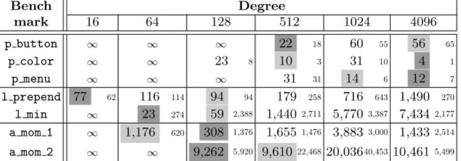
Bench Degree mark 16 64 128 512 1024 4096 p button ∞ ∞ ∞ 22 18 60 55 56 65 p color ∞ ∞ 23 8 10 3 31 10 4 1 p menu ∞ ∞ ∞ 31 31 14 6 12 7 l prepend 77 62 116 114 94 94 179 258 716 643 1,490 270 l min ∞ 23 274 59 2,388 1,440 2,711 5,7703,387 7,434 2,177 a mom 1 ∞ 1,176 620 308 1,376 1,655 1,476 3,8833,000 1,433 2,514 a mom 2 ∞ ∞ 9,262 5,920 9,61022,46820,03640,45310,461 5,499
Table 1: Expected running time (s) using empirical success rate. SIQR in small text. Fastest time in dark grey, second-fastest in light grey.
synthesis domains. The left column of Table 1 lists the benchmarks, grouped by domain. Section 5.1 describes the programs and experimental machine in more detail. We ran each benchmark with degrees varying exponentially from 16 to 4096. For each degree, we ran each benchmark 256 times, with no timeout.
For each benchmark/degree pair, we wish to estimate the time to success if we concretized the same benchmark many times at that degree. To form this estimate, for each such pair we compute the fraction of runs p that succeeded; this approximates the true probability of success. Then if a trial takes time t, we compute the expected time to success as t/p. While this is a coarse estimate, it provides a simple calculation we can also use in an algorithm (Section 4). If p is 0 (no trial succeeded), the expected time to success is ∞.
Results. Each cell in Table 1 contains the median expected run time in sec-onds, as computed for each degree. Since variance is high, we also report the semi-interquartile range (SIQR) of the running times, shown in small text. We highlight the fastest and second-fastest times.
The table shows that the optimal degree varies across all benchmarks; indeed, all degrees except 1024 were optimal for at least one benchmark. We also see a lot of variance across runs. For example, for l min, degree 128, the SIQR is more than 40× the median. Other benchmarks also have high SIQRs. Importantly, if we visualize the median expected running times, they form a vee around the fastest time—performance gets worse the farther away from optimal in either direction. Thus, we can search for an optimal degree, as we discuss next.
4
Adaptive, Parallel Concretization
Figure 1 gives pseudocode for adaptive concretization. The core step of our algorithm, encapsulated in the run trial function, is to run Sketch with the
specified degree. If a solution is found, we exit the search. Otherwise, we return both the time taken by that trial and the size of the concretization space, e.g., if we concretized n bits, we return 2n. We will use this information to estimate
run trial(degree)
run Sketch with specified degree if solution found then
raise success else
return (running time,
concretization space size )
compare(deg a, deg b) dist a ← ∅
dist b ← ∅
while |dist a | ≤ Max dist ∧ wilcoxon(dist a, dist b ) > T do dist a ∪ ← run trial(deg a) dist b ∪ ← run trial(deg b) if wilcoxon(dist a, dist b ) > T then
return tie
elsif avg( dist a ) < avg(dist b) then return left
else
return right
climb()
low, high ← 0, 1
while high < Max exp do case compare(2low, 2high) of
left : break right:
low ← high high ← high + 1 tie : high ← high + 1 return (low, high)
bin search(low, high) mid ← (low + high) / 2 case compare(low, mid) of
left : return bin search(low, mid) right: return bin search(mid, high) tie : return mid
main()
(low, high) ← climb()
deg ← bin search(2low, 2high) while (true) do run trial(deg)
Fig. 1: Search Algorithm using Wilcoxon Signed-Rank Test.
Since Sketch solving has some randomness in it, a single trial is not enough to provide a good estimate of time-to-solution, even under our heuristic assump-tions. In Table 1 we used 256 trials at each degree, but for a practical algorithm, we cannot fix a number of trials, lest we run either too many trials (which wastes time) or too few (which may give a non-useful result).
To solve this issue, our algorithm uses the Wilcoxon Signed-Rank Test [24] to determine when we have enough data to distinguish two degrees. We assume we have a function wilcoxon(dist a, dist b ) that takes two equal-length lists of (time, concretization space size) pairs, converts them to distributions of esti-mated times-to-solution, and implements the test, returning a p-value indicating the probability that the means of the two distributions are different.
Recall that in our preliminary experiment in Section 3, we calculated the estimated time to success of each trial as t/p, where t was the time of the trial and p was the empirical probability of success. We use the same calculation in this algorithm, except we need a different way to compute p, since the success rate is always 0 until we find a solution, at which point we stop. Thus, we instead calculate p from the search space size. We assume there is only one solution, so if the search space size is s, we calculate p = 1/s.4
4
Notice we can ignore the size of the symbolic space, since symbolic search will find a solution if one exists for the particular concretization.
Comparing Degrees. Next, comparetakes two degrees as inputs and returns a value indicating whether the left argument has lower expected running time, therightargument does, or it is atie. The function initially creates two empty sets of trial results, dist a and dist b. Then it repeatedly callsrun trialto add a new trial to each of the two distributions (we write x ∪ ← yto mean adding y to set x). Iteration stops when the number of elements in each set exceeds some thresholdMax dist, or thewilcoxonfunction returns a p-value below some threshold T . Once the algorithm terminates, we return tieif the threshold was never reached, or left orrightdepending on the means.
In our experiments, we use 3 × max(8, |cores|) forMax dist. Thus,compare
runs at most three “rounds” of at least eight samples (or the number of cores, if that is larger). This lets us cut off the comparefunction if it does not seem to be finding any distinction. We use 0.2 for the threshold T . This is higher than a typical p-value (which might be 0.05), but recall our algorithm is such that returning an incorrect answer will only affect performance and not correctness. We leave it to future work to tuneMax dist andTfurther.
Searching for the Optimal Degree. Given the comparesubroutine, we can im-plement the search algorithm. The entry point ismain, shown in the lower-right corner of Figure 1. There are two algorithm phases: an exponential climbing phase (function climb) in which we try to roughly bound the optimal degree, followed by a binary search (functionbin search) within those bounds.
We opted for an initial exponential climb because binary search across the whole range could be extremely slow. Consider the first iteration of such a pro-cess, which would compare full concretization against no concretization. While the former would complete almost instantaneously, the latter could potentially take a long time (especially in situations when our algorithm is most useful).
Theclimbfunction aims to return a pairlow,highsuch that the optimal de-gree is between 2lowand 2high. It begins withlowandhighas 0 and 1, respectively. It then increases both variables until it finds values such that at degree 2high, search is estimated to take a longer time than at 2low, i.e., making things more symbolic thanlowcauses too much slowdown. Notice that the initial trials of the
climbwill be extremely fast, because almost all variables will be concretized. To perform this search,climbrepeatedly callscompare, passing in 2 to the power oflowand highas the degrees to compare. Then there are three cases. If
left is returned, 2low has better expected running time than 2high. Hence we assume the true optimal degree is somewhere between the two, so we return them. Otherwise, ifrightis returned, then 2high is better than 2low, so we shift up to the next exponential range. Finally, if it is a tie, then the range is too narrow to show a difference, so we widen it by leavinglowalone and incrementinghigh. We also terminate climbing if highexceeds some maximum exponent Max exp. In our implementation, we chooseMax expas 14, since for our subject programs this makes runs nearly all symbolic.
After finding rough bounds with climb, we then continue with a binary search. Notice that inbin search,lowandhighare the actual degrees, whereas in
the invariant that low has expected faster or equivalent solution time to high
(recall this is established by climb). Thus each iteration picks a midpoint mid
and determines whether lowis better than mid, in which case midbecomes the newhigh; ormidis better, in which case the range shifts tomidtohigh; or there is no difference, in which casemidis returned as the optimal degree.
Finally, after the degree search has finished, we repeatedly run Sketch with the given degree. The search exits when run trial finds a solution, which it signals by raising an exception to exit the algorithm. (Note thatrun trialmay find a solution at any time, including duringclimbor bin search).
Parallelization. Our algorithm is easy to parallelize. The natural place to do this is insiderun trial: Rather than run a single trial at a time, we perform parallel trials. More specifically, our implementation includes a worker pool of a user-specified size. Each worker performs concretization randomly at the user-specified degree, and thus they are highly likely to all be doing distinct work.
Timeouts. Like all synthesis tools, Sketch includes a timeout that kills a search that seems to be taking too long. Timeouts are tricky to get right, because it is hard to know whether a slightly longer run would have succeeded. Our algorithm exacerbates this problem because it runs many trials. If those trials are killed just short of the necessary time, it adds up to a lot of wasted work. At the other extreme, we could have no timeout, but then the algorithm may also waste a lot of time, e.g., searching for a solution with incorrectly concretized values.
To mitigate the disadvantages of both extremes, our implementation uses an adaptive timeout. All worker threads share an initial timeout value of one minute. When a worker thread hits a timeout, it stops, but it doubles the shared timeout value. In this way, we avoid getting stuck rerunning with too short a timeout. Note that we only increase the timeout duringclimband bin search. Once we fix the degree, we leave the timeout fixed.
5
Experimental Evaluation
We empirically evaluated adaptive concretization against a range of benchmarks with various characteristics.5
Compared to regular Sketch (i.e., pure symbolic search), we found our algorithm is substantially faster in many cases; competi-tive in most of the others; and slower on a few benchmarks. We also compared adaptive concretization with concretization fixed at the final degree chosen by the adaption phase of our algorithm (i.e., to see what would happen if we could guess this in advance), and we found performance is reasonably close, mean-ing the overhead for adaptation is not high. We measured parallel scalability of adaptive concretization of 1, 4, and 32 cores, and found it generally scales well. We also compared against the winner of the SyGuS’14 competition on a subset
5
Our testing infrastructure, benchmarks, and raw experimental data are open-sourced and explained at: http://plum-umd.github.io/adaptive-concretization/.
of the benchmarks and found that adaptive concretization is better than the winner on 6 of 9 benchmarks and competitive on the remaining benchmarks.
Throughout this section, all performance reports are based on 13 runs on a server equipped with forty 2.4 GHz Intel Xeon processors and 99 GB RAM, running Ubuntu 14.04.1. LTS. (We used the same machine for the experiments in Section 3.) For the pure Sketch runs only, performance is also on 13 runs with a 2-hour timeout and 32 GB memory bound.
5.1 Benchmarks
The names of our benchmarks are listed in the left column of Table 2, with the size in the next column. The benchmarks are grouped by the synthesis appli-cation they are from. Each appliappli-cation domain’s sketches vary in complexity, amount of symmetry, etc. We discuss the groups in order.
– Pasket. The first three benchmarks, beginning with p , come from the appli-cation that inspired this work: Pasket, a tool that aims to construct executable code that behaves the same as a framework such as Java Swing, but is much simpler to statically analyze [11]. Pasket’s sketches are some of the largest that have ever been tried, and we developed adaptive concretization because they were initially intractable with Sketch. As benchmarks, we selected three Pas-ket sPas-ketches that aim to synthesize parts of Java Swing that include buttons, the color chooser, and menus.
– Data Structure Manipulation. The second set of benchmarks is from a project aiming to synthesize provably correct data-structure manipulations [13]. Each synthesis problem consists of a program template and logical specifications de-scribing the functional correctness of the expected program. There are two bench-marks. l prepend accepts a sorted singly linked list L and prepends a key k, which is smaller than any element in L. l min traverses a singly linked list via a while loop and returns the smallest key in the list.
– Invariants for Stencils. The next sets of benchmarks, beginning with a mom , are from a system that synthesizes invariants and postconditions for scientific computations involving stencils. In this case, the stencils come from a DOE Miniapp called Cloverleaf [7]. These benchmarks involve primarily integer arith-metic and large numbers of loops.
– SyGuS Competition. The next sets of benchmarks, beginning with ar and hd , are from the first Syntax-Guided Synthesis Competition [1], which compared synthesizers using a common set of benchmarks. We selected nine benchmarks that took at least 10 seconds for any of the solvers in the competition, but at least one solver was able to solve it.
– Sketch. The last three groups of benchmarks, beginning with s , deriv, and q , are from Sketch’s performance test suite, which is used to identify perfor-mance regressions in Sketch and measure potential benefits of optimizations.
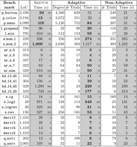
Bench Sketch Adaptive Non-Adaptive mark LoC Time (s) Degree # Trials Time (s) # Trials Time (s) p button 3,436 50 ∞ 4,160 639 51 8 249 21 6 p color 3,194 13 0 3,072 551 33 6 109 12 4 p menu 4,099 OOM 5,120 752 84 18 207 31 10 l prepend 708 96 8 32 98 20 4 110 25 4 l min 795 810 235 512 153 59 40 17 28 6 a mom 1 229 336 35 256 316 274 76 331 285 16 a mom 2 231 1,000 56 2,048 383 1,517 254 303 1,422 89 ar s 4 313 6 1 16 18 3 0 25 3 0 ar s 5 334 9 0 16 17 4 0 29 4 1 ar s 6 337 17 2 32 23 6 0 33 9 1 ar s 7 322 63 8 64 84 50 12 35 59 8 ar sum 328 618 282 16 11 50 19 27 31 8 hd 13 d5 310 88 47 16 3 11 2 7 8 0 hd 14 d1 304 156 41 16 5 29 12 10 22 7 hd 14 d5 329 1,294 388 16 23 229 47 16 239 83 hd 15 d5 329 733 370 32 9 177 16 6 213 39 s cg 124 18 4 64 161 15 2 160 14 0 s log2 49 971 314 128 114 349 105 25 131 89 s logcnt 30 225 206 32 90 21 26 84 16 6 s rev 136 327 202 256 165 53 22 11 43 14 deriv2 1,444 28 4 16 15 8 0 20 8 2 deriv3 1,410 28 2 32 9 7 1 10 7 0 deriv4 1,410 14 0 16 7 6 0 20 5 0 deriv5 1,410 14 1 16 7 6 0 19 5 0 q noti 262 12 6 32 100 8 2 79 6 1 q serv 2,005 105 60 32 11 22 2 9 23 2
Table 2: Comparing Sketch, adaptive, and non-adaptive concretization. 5.2 Performance Results
The right columns of Table 2 show our results. The columns that include running time are greyed for easy comparison, with the semi-interquartile range (SIQR) in a small font. (We only list the running times SIQR to save space.) The median is ∞ if more than half the runs timed out, while the SIQR is ∞ if more than one quarter of the runs timed out. The first grey column lists Sketch’s running time on one core. The next group of columns reports on adaptive concretization, run on 32 cores. The first column in the group gives the median of the final degrees chosen by adaptive concretization. The next column lists the median number of calls to run trial. The last column lists the median running time. Lastly, the right group of columns shows the performance of our algorithm on 32 cores, assuming we skip the adaptation step and jump straight to running with the median degree shown in the table. For example, for p button, these columns report results for running starting with degree 4,160 and never changing it. We again report the number of trials and the running time.
Comparing Sketch and adaptive concretization, we find that adaptive con-cretization typically performs better. In the figure, we boldface the fastest time between those two columns. We see several significant speedups, ranging from 14× for l min, 12× for ar sum, and 11× for s logcnt to 4× for hd 15 d5 and deriv3 and 3× for ar s 6 and s log2. For p button, regular Sketch reaches the 2-hour timeout in 4 of 13 runs, while our algorithm succeeds, mostly within one minute. In another case, p menu, Sketch reliably exceeds our 32GB mem-ory bound and then aborts. Overall, adaptive concretization performed better in 23 of 26 benchmarks, and about the same on one benchmark.
On the remaining benchmarks (p color and a mom 2), adaptive concretiza-tion’s performance was within about a factor of two. Comparing other similarly short-running benchmarks, such as deriv4 and deriv5, where the final degree (16) was chosen very early, the degree search process needed to spend more time to reach bigger degree, resulting in the slowdown. Finally, a mom 2 is 1.5× slower. In this case, Sketch’s synthesis phase is extremely fast, hence parallelization has no benefit. Instead, the running time is dominated by the checking phase (when the candidate solution is checked symbolically against all possible inputs), and using adaptive concretization only adds overhead.
Next we compare adaptive concretization to non-adaptive concretization at the final degree. In 7 cases, the adaptive algorithm is actually faster, due to random chance. In the remaining cases, the adaptive algorithm is either about the same as non-adaptive or is at worst within a factor of approximately three.
5.3 Parallel Scalability and Comparison to SyGuS Solvers
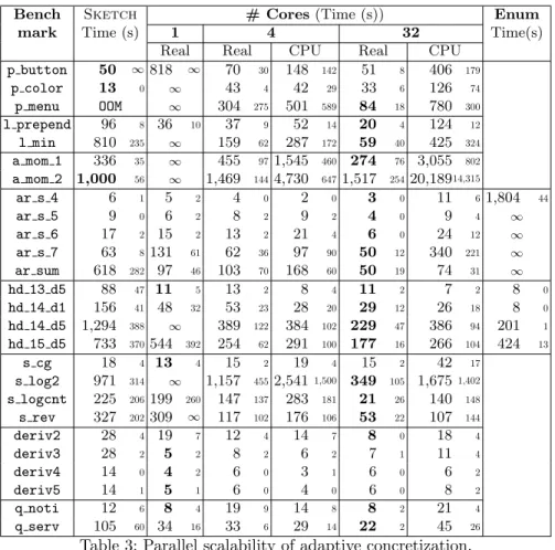
We next measured how adaptive concretization’s performance varies with the number of cores, and compare it to the winner of the SyGuS competition. Table 3 shows the results. The first two columns are the same as Table 2. The next five columns show the performance of adaptive concretization on 1, 4, and 32 cores. Real time is wall-clock time for the parallel run (the 32-core real-time column is the same as Table 2), and CPU time is the cumulative Sketch back-end time summed over all cores. We discuss the rightmost column shortly. We boldface the fastest real time among Sketch, 1, 4, and 32 cores.
The real-time results show that, in the one-core experiments, adaptive con-cretization performs better than regular Sketch in 17 of 26 cases. Although adaptive concretization is worse or times out in the other cases, its performance improves with the number of cores. The 4-core runs are consistently close to or better than 1-core runs; in some cases, benchmarks that time out on 1 core succeed on 4 cores. At 32 cores, we see the best performance in 20 of the 26 cases, with a speedup over 4-core runs ranging up to 7×. There is only one case where 4 cores is faster than 32: a mom 2. However, as the close medians and large SIQR indicate, this is noise due to randomness in Sketch.
Comparing real times and CPU time, we can see that our algorithm does fully utilize all cores. Investigating further, we found one source of overhead is that each trial re-loads its input file. We plan to eliminate this cost in the future by only reading the input once and then sharing the resulting data structure.
Bench Sketch # Cores (Time (s)) Enum mark Time (s) 1 4 32 Time(s)
Real Real CPU Real CPU p button 50 ∞818 ∞ 70 30 148 142 51 8 406 179 p color 13 0 ∞ 43 4 42 29 33 6 126 74 p menu OOM ∞ 304 275 501 589 84 18 780 300 l prepend 96 8 36 10 37 9 52 14 20 4 124 12 l min 810 235 ∞ 159 62 287 172 59 40 425 324 a mom 1 336 35 ∞ 455 971,545 460 274 76 3,055 802 a mom 2 1,000 56 ∞ 1,469 1444,730 6471,517 25420,18914,315 ar s 4 6 1 5 2 4 0 2 0 3 0 11 6 1,804 44 ar s 5 9 0 6 2 8 2 9 2 4 0 9 4 ∞ ar s 6 17 2 15 2 13 2 21 4 6 0 24 12 ∞ ar s 7 63 8131 61 62 36 97 90 50 12 340 221 ∞ ar sum 618 282 97 46 103 70 168 60 50 19 74 31 ∞ hd 13 d5 88 47 11 5 13 2 8 4 11 2 7 2 8 0 hd 14 d1 156 41 48 32 53 23 28 20 29 12 26 18 8 0 hd 14 d5 1,294 388 ∞ 389 122 384 102 229 47 386 94 201 1 hd 15 d5 733 370544 392 254 62 291 100 177 16 266 104 424 13 s cg 18 4 13 4 15 2 19 4 15 2 42 17 s log2 971 314 ∞ 1,157 4552,5411,500 349 105 1,675 1,402 s logcnt 225 206199 260 147 137 283 181 21 26 140 148 s rev 327 202309 ∞ 117 102 176 106 53 22 107 144 deriv2 28 4 19 7 12 4 14 7 8 0 18 4 deriv3 28 2 5 2 8 2 6 2 7 1 11 4 deriv4 14 0 4 2 6 0 3 1 6 0 6 2 deriv5 14 1 5 1 6 0 4 0 6 0 8 2 q noti 12 6 8 4 19 9 14 8 8 2 21 4 q serv 105 60 34 16 33 6 29 14 22 2 45 26
Table 3: Parallel scalability of adaptive concretization.
Finally, the rightmost column of Table 3 shows the performance of the merative CEGIS Solver, which won the SyGuS’14 Competition [1]. As the Enu-merative Solver does not accept problems in Sketch format, we only compare on benchmarks from the competition (which uses the SyGuS-IF format, which is easily translated to a sketch). We should note that the enumerative solver is not parallelized and may be difficult to parallelize.
Adaptive concretization is faster for 6 of 9 benchmarks from the competition. It is also worth mentioning the Enumerative Solver actually won on the four benchmarks beginning with hd . Our results show that adaptive concretization outperforms it on one benchmark and is competitive on the others.
6
Related Work
There have been many recent successes in sampling-based synthesis techniques. For example, Schkufza et al. use sampling-based synthesis for optimization [14, 15], and Sharma et al. use similar techniques to discover complex invariants in programs [16]. These systems use Markov Chain Montecarlo (MCMC)
tech-niques, which use fitness functions to prioritize sampling over regions of the solution space that are more promising. This is more sophisticated sampling technique than what is used by our method. We leave it to future work to ex-plore MCMC methods in our context. Another alternative to constraint-based synthesis is explicit enumeration of candidate solutions. Enumerative solvers of-ten rely on factoring the search space, aggressive pruning and lattice search. Factoring has been very successful for programming by example [8, 10, 17], and lattice search has been used in synchronization of concurrent data structures [23] and autotuning [2]. However, both factoring and lattice search require signifi-cant domain knowledge, so they are unsuitable for a general purpose system like Sketch. Pruning techniques are more generally applicable, and are used aggressively by the enumerative solver compared against in Section 5.
Recently, some researchers have explored ways to use symbolic reasoning to improve sampling-based procedures. For example, Chaudhuri et al. have shown how to use numerical search for synthesis by applying a symbolic smoothing transformation [4, 5]. In a similar vein, Chaganty et al. use symbolic reasoning to limit the sampling space for probabilistic programs to exclude points that will not satisfy a specification [3]. We leave exploring the tradeoffs between these approaches as future work.
Finally, there has been significant interest in parallelizing SAT/SMT solvers. The most successful of these combine a portfolio approach—solvers are run in parallel with different heuristics—with clause sharing [9, 25]. Interestingly, these solvers are more efficient than solvers like PSATO [26] where every thread ex-plores a subset of the space. One advantage of our approach over solver paral-lelization approaches is that the concretization happens at a very high-level of abstraction, so the solver can apply aggressive algebraic simplification based on the concretization. This allows our approach to even help a problem like p menu that ran out of memory on the sequential solver. The tradeoff is that our solver loses the ability to tell if a problem is UNSAT because we cannot distinguish not finding a solution from having made incorrect guesses during concretization.
7
Conclusion
We introduced adaptive concretization, a program synthesis technique that com-bines explicit and symbolic search. Our key insight is that not all unknowns are equally important with respect to solving time. By concretizing high influence unknowns, we can often speed up the overall synthesis algorithm, especially when we add parallelism. Since the best degree of concretization is hard to compute, we presented an online algorithm that uses exponential hill climbing and bi-nary search to find a suitable degree by running many trials. We implemented our algorithm for Sketch and ran it on a suite of 26 benchmarks across sev-eral different domains. We found that adaptive concretization often outperforms Sketch, sometimes very significantly. We also found that the parallel scalability of our algorithm is reasonable.
References
1. Alur, R., Bod´ık, R., Juniwal, G., Martin, M.M.K., Raghothaman, M., Seshia, S.A., Singh, R., Solar-Lezama, A., Torlak, E., Udupa, A.: Syntax-guided synthe-sis. In: Formal Methods in Computer-Aided Design, FMCAD 2013, Portland, OR, USA, October 20-23, 2013. pp. 1–17 (2013), http://ieeexplore.ieee.org/xpl/ freeabs_all.jsp?arnumber=6679385
2. Ansel, J., Kamil, S., Veeramachaneni, K., Ragan-Kelley, J., Bosboom, J., O’Reilly, U., Amarasinghe, S.P.: Opentuner: an extensible framework for program auto-tuning. In: International Conference on Parallel Architectures and Compilation, PACT ’14, Edmonton, AB, Canada, August 24-27, 2014. pp. 303–316 (2014), http://doi.acm.org/10.1145/2628071.2628092
3. Chaganty, A., Nori, A.V., Rajamani, S.K.: Efficiently sampling probabilistic pro-grams via program analysis. In: Proceedings of the Sixteenth International Con-ference on Artificial Intelligence and Statistics, AISTATS 2013, Scottsdale, AZ, USA, April 29 - May 1, 2013. pp. 153–160 (2013), http://jmlr.org/proceedings/ papers/v31/chaganty13a.html
4. Chaudhuri, S., Clochard, M., Solar-Lezama, A.: Bridging boolean and quantitative synthesis using smoothed proof search. In: The 41st Annual ACM SIGPLAN-SIGACT Symposium on Principles of Programming Languages, POPL ’14, San Diego, CA, USA, January 20-21, 2014. pp. 207–220 (2014), http://doi.acm.org/ 10.1145/2535838.2535859
5. Chaudhuri, S., Solar-Lezama, A.: Smooth interpretation. In: Proceedings of the 2010 ACM SIGPLAN Conference on Programming Language Design and Imple-mentation, PLDI 2010, Toronto, Ontario, Canada, June 5-10, 2010. pp. 279–291 (2010), http://doi.acm.org/10.1145/1806596.1806629
6. Cheung, A., Solar-Lezama, A., Madden, S.: Optimizing database-backed appli-cations with query synthesis. In: ACM SIGPLAN Conference on Programming Language Design and Implementation, PLDI ’13, Seattle, WA, USA, June 16-19, 2013. pp. 3–14 (2013), http://doi.acm.org/10.1145/2462156.2462180
7. Gaudin, W., Mallinson, A., Perks, O., Herdman, J., Beckingsale, D., Levesque, J., Jarvis, S.: Optimising hydrodynamics applications for the cray xc30 with the application tool suite. The Cray User Group pp. 4–8 (2014)
8. Gulwani, S.: Automating string processing in spreadsheets using input-output ex-amples. In: Proceedings of the 38th ACM SIGPLAN-SIGACT Symposium on Prin-ciples of Programming Languages, POPL 2011, Austin, TX, USA, January 26-28, 2011. pp. 317–330 (2011), http://doi.acm.org/10.1145/1926385.1926423 9. Hamadi, Y., Jabbour, S., Sais, L.: Manysat: a parallel SAT solver. JSAT 6(4), 245–
262 (2009), http://jsat.ewi.tudelft.nl/content/volume6/JSAT6_12_Hamadi. pdf
10. Harris, W.R., Gulwani, S.: Spreadsheet table transformations from examples. In: Proceedings of the 32nd ACM SIGPLAN Conference on Programming Language Design and Implementation, PLDI 2011, San Jose, CA, USA, June 4-8, 2011. pp. 317–328 (2011), http://doi.acm.org/10.1145/1993498.1993536
11. Jeon, J., Qiu, X., Foster, J.S., Solar-Lezama, A.: Synthesizing Framework Models for Symbolic Execution, under submission
12. Jha, S., Gulwani, S., Seshia, S.A., Tiwari, A.: Oracle-guided component-based pro-gram synthesis. In: Proceedings of the 32nd ACM/IEEE International Conference on Software Engineering - Volume 1. pp. 215–224. ICSE ’10, ACM, New York, NY, USA (2010), http://doi.acm.org/10.1145/1806799.1806833
13. Qiu, X., Solar-Lezama, A.: Synthesizing Data-Structure Manipulations with Nat-ural Proofs, under submission
14. Schkufza, E., Sharma, R., Aiken, A.: Stochastic superoptimization. In: Architec-tural Support for Programming Languages and Operating Systems, ASPLOS ’13, Houston, TX, USA - March 16 - 20, 2013. pp. 305–316 (2013), http://doi.acm. org/10.1145/2451116.2451150
15. Schkufza, E., Sharma, R., Aiken, A.: Stochastic optimization of floating-point pro-grams with tunable precision. In: ACM SIGPLAN Conference on Programming Language Design and Implementation, PLDI ’14, Edinburgh, United Kingdom -June 09 - 11, 2014. p. 9 (2014), http://doi.acm.org/10.1145/2594291.2594302 16. Sharma, R., Aiken, A.: From invariant checking to invariant inference using
ran-domized search. In: Computer Aided Verification - 26th International Conference, CAV 2014, Held as Part of the Vienna Summer of Logic, VSL 2014, Vienna, Aus-tria, July 18-22, 2014. Proceedings. pp. 88–105 (2014), http://dx.doi.org/10. 1007/978-3-319-08867-9_6
17. Singh, R., Gulwani, S.: Synthesizing number transformations from input-output examples. In: Computer Aided Verification - 24th International Conference, CAV 2012, Berkeley, CA, USA, July 7-13, 2012 Proceedings. pp. 634–651 (2012), http: //dx.doi.org/10.1007/978-3-642-31424-7_44
18. Singh, R., Gulwani, S., Solar-Lezama, A.: Automated feedback generation for intro-ductory programming assignments. In: ACM SIGPLAN Conference on Program-ming Language Design and Implementation, PLDI ’13, Seattle, WA, USA, June 16-19, 2013. pp. 15–26 (2013), http://doi.acm.org/10.1145/2462156.2462195 19. Solar-Lezama, A.: Program sketching. International Journal on Software Tools for
Technology Transfer 15(5-6), 475–495 (2013)
20. Solar-Lezama, A., Jones, C.G., Bodik, R.: Sketching concurrent data structures. In: Proceedings of the 2008 ACM SIGPLAN conference on Programming language design and implementation. pp. 136–148. PLDI ’08 (2008)
21. Torlak, E., Bod´ık, R.: A lightweight symbolic virtual machine for solver-aided host languages. In: ACM SIGPLAN Conference on Programming Language Design and Implementation, PLDI ’14, Edinburgh, United Kingdom - June 09 - 11, 2014. p. 54 (2014), http://doi.acm.org/10.1145/2594291.2594340
22. Udupa, A., Raghavan, A., Deshmukh, J.V., Mador-Haim, S., Martin, M.M.K., Alur, R.: TRANSIT: specifying protocols with concolic snippets. In: ACM SIG-PLAN Conference on Programming Language Design and Implementation, PLDI ’13, Seattle, WA, USA, June 16-19, 2013. pp. 287–296 (2013), http://doi.acm. org/10.1145/2462156.2462174
23. Vechev, M.T., Yahav, E.: Deriving linearizable fine-grained concurrent objects. In: Proceedings of the ACM SIGPLAN 2008 Conference on Programming Lan-guage Design and Implementation, Tucson, AZ, USA, June 7-13, 2008. pp. 125–135 (2008), http://doi.acm.org/10.1145/1375581.1375598
24. Wilcoxon, F.: Individual Comparisons by Ranking Methods. Biometrics Bulletin 1(6), 80–83 (1945)
25. Wintersteiger, C.M., Hamadi, Y., de Moura, L.M.: A concurrent portfolio approach to SMT solving. In: Computer Aided Verification, 21st International Conference, CAV 2009, Grenoble, France, June 26 - July 2, 2009. Proceedings. pp. 715–720 (2009), http://dx.doi.org/10.1007/978-3-642-02658-4_60
26. Zhang, H., Bonacina, M.P., Hsiang, J.: Psato: A distributed propositional prover and its application to quasigroup problems. J. Symb. Comput. 21(4-6), 543–560 (Jun 1996), http://dx.doi.org/10.1006/jsco.1996.0030