A COORDINATED X-RAY AND OPTICAL CAMPAIGN
OF THE NEAREST MASSIVE ECLIPSING BINARY, #
ORIONIS Aa. I. OVERVIEW OF THE X-RAY SPECTRUM
The MIT Faculty has made this article openly available.
Please share
how this access benefits you. Your story matters.
Citation
Corcoran, M. F., J. S. Nichols, H. Pablo, T. Shenar, A. M. T. Pollock,
W. L. Waldron, A. F. J. Moffat, et al. “A COORDINATED X-RAY AND
OPTICAL CAMPAIGN OF THE NEAREST MASSIVE ECLIPSING
BINARY, δ ORIONIS Aa. I. OVERVIEW OF THE X-RAY SPECTRUM.”
The Astrophysical Journal 809, no. 2 (August 19, 2015): 132. © 2015
The American Astronomical Society
As Published
http://dx.doi.org/10.1088/0004-637x/809/2/132
Publisher
IOP Publishing
Version
Final published version
Citable link
http://hdl.handle.net/1721.1/99913
Terms of Use
Article is made available in accordance with the publisher's
policy and may be subject to US copyright law. Please refer to the
publisher's site for terms of use.
A COORDINATED X-RAY AND OPTICAL CAMPAIGN OF THE NEAREST MASSIVE ECLIPSING BINARY,
δ ORIONIS Aa. I. OVERVIEW OF THE X-RAY SPECTRUM
M. F. Corcoran1,2, J. S. Nichols3, H. Pablo4, T. Shenar5, A. M. T. Pollock6, W. L. Waldron7, A. F. J. Moffat4, N. D. Richardson4, C. M. P. Russell8, K. Hamaguchi1,9, D. P. Huenemoerder10, L. Oskinova5, W.-R. Hamann5, Y. Nazé11,22, R. Ignace12, N. R. Evans13, J. R. Lomax14, J. L. Hoffman15, K. Gayley16, S. P. Owocki17, M. Leutenegger1,9, T. R. Gull18,
K. T. Hole19, J. Lauer3, and R. C. Iping20,21
1
CRESST and X-ray Astrophysics Laboratory, NASA/Goddard Space Flight Center, Greenbelt, MD 20771, USA;michael.f.corcoran@nasa.gov
2
Universities Space Research Association, 7178 Columbia Gateway Drive, Columbia, MD 21044, USA 3
Harvard-Smithsonian Center for Astrophysics, 60 Garden Street, MS 34, Cambridge, MA 02138, USA 4
Département de physique and Centre de Recherche en Astrophysique du Québec(CRAQ), Université de Montréal, C.P. 6128, Succ. Centre-Ville, Montréal, Québec, H3C 3J7, Canada
5
Institut für Physik und Astronomie, Universität Potsdam, Karl-Liebknecht-Str. 24/25, D-14476 Potsdam, Germany 6
European Space Agency, XMM-Newton Science Operations Centre, European Space Astronomy Centre, Apartado 78, E-28691 Villanueva de la Cañada, Spain 7Eureka Scientific, Inc., 2452 Delmer St., Oakland, CA 94602, USA
8
NASA-GSFC, Code 662, Goddard Space Flight Center, Greenbelt, MD, 20771 USA 9
Department of Physics, University of Maryland, Baltimore County, 1000 Hilltop Circle, Baltimore, MD 21250, USA 10
Massachusetts Institute of Technology, Kavli Institute for Astrophysics and Space Research, 77 Massachusetts Avenue, Cambridge, MA 02139 USA 11Groupe d’Astrophysique des Hautes Energies, Institut d’Astrophysique et de Géophysique, Université de Liége,
17, Allée du 6 Août, B5c, B-4000 Sart Tilman, Belgium 12
Physics and Astronomy, East Tennessee State University, Johnson City, TN 37614, USA 13
Harvard-Smithsonian Center for Astrophysics, 60 Garden Street, MS 4, Cambridge, MA 02138, USA 14
Homer L. Dodge Department of Physics and Astronomy, University of Oklahoma, 440 W Brooks Street, Norman, OK, 73019 USA 15
Department of Physics and Astronomy, University of Denver, 2112 E. Wesley Avenue, Denver, CO, 80208 USA 16
Department of Physics and Astronomy, University of Iowa, Iowa City, IA 52242, USA 17
University of Delaware, Bartol Research Institute, Newark, DE 19716, USA 18
Laboratory for Extraterrestrial Planets and Stellar Astrophysics, Code 667, NASA/Goddard Space Flight Center, Greenbelt, MD 20771, USA 19
Department of Physics, Weber State University, 2508 University Circle, Ogden, UT 84408, USA 20
CRESST and Observational Cosmology Laboratory, NASA/Goddard Space Flight Center, Greenbelt, MD 20771, USA 21
Department of Astronomy, University of Maryland, 1113 Physical Sciences Complex, College Park, MD 20742-2421, USA Received 2014 December 29; accepted 2015 March 31; published 2015 August 18
ABSTRACT
We present an overview of four deep phase-constrained Chandra HETGS X-ray observations of δ Ori A. Delta Ori A is actually a triple system that includes the nearest massive eclipsing spectroscopic binary,δ Ori Aa, the only such object that can be observed with little phase-smearing with the Chandra gratings. Since the fainter star,δ Ori Aa2, has a much lower X-ray luminosity than the brighter primary (δ Ori Aa1), δ Ori Aa provides a unique system with which to test the spatial distribution of the X-ray emitting gas aroundδ Ori Aa1 via occultation by the photosphere of, and wind cavity around, the X-ray dark secondary. Here we discuss the X-ray spectrum and X-ray line profiles for the combined observation, having an exposure time of nearly 500 ks and covering nearly the entire binary orbit. The companion papers discuss the X-ray variability seen in the Chandra spectra, present new space-based photometry and ground-based radial velocities obtained simultaneously with the X-ray data to better constrain the system parameters, and model the effects of X-rays on the optical and UV spectra. Wefind that the X-ray emission is dominated by embedded wind shock emission from star Aa1, with little contribution from the tertiary star Ab or the shocked gas produced by the collision of the wind of Aa1 against the surface of Aa2. Wefind a similar temperature distribution to previous X-ray spectrum analyses. We also show that the line half-widths are about 0.3−0.5 times the terminal velocity of the wind of star Aa1. We find a strong anti-correlation between line widths and the line excitation energy, which suggests that longer-wavelength, lower-temperature lines form farther out in the wind. Our analysis also indicates that the ratio of the intensities of the strong and weak lines of FeXVII
and NeXare inconsistent with model predictions, which may be an effect of resonance scattering.
Key words: binaries: close– binaries: eclipsing – stars: early-type – stars: individual (Delta Ori) – stars: mass-loss – X-rays: stars
1. INTRODUCTION
Massive O-type stars, though rare, are primary drivers of the chemical, ionization, and pressure evolution of the interstellar medium. The evolution of these stars from the main sequence to supernova depends on their mass and is significantly affected by stellar wind mass loss. Our best estimates of mass, radius, and luminosity for O stars come from direct dynamical
analyses of photometric and radial velocity variations in massive, eclipsing binaries. However, because massive stars are rare and massive binaries that have been studied in detail are rarer still(of the 2386 systems listed in the Ninth Catalog of Spectroscopic Binaries, only 82 of them have O-type components), direct dynamical determinations of stellar parameters are only known for a few systems.
Current uncertainties regarding the amount and distribution of mass lost through stellar winds are even larger, since it is difficult to determine stellar wind parameters in a direct,
© 2015. The American Astronomical Society. All rights reserved.
22
model-independent way. Radiatively driven stellar winds have mass-loss rates of M˙ ~10-5-10-7 Myr−1 (for a
review, see Kudritzki & Puls 2000). However,
observation-ally determined mass-loss rates have been estimated, in many, if not most cases, using an idealized smooth, spherically symmetric wind. Stellar winds are probably not spherical; variations of photospheric temperature with latitude are inevitable because of stellar rotation (and tidal deformation of stars in binaries), and these temperature variations will produce latitudinally dependent wind densities and velocities (Owocki et al.1996). Stellar winds are not smooth either; the
radiative driving force is inherently unstable to small velocity perturbations, and wind instabilities are expected to grow into dense structures (clumps) distributed through the wind. In addition, clumps can also be produced by sub-surface convective zones in massive stars caused by opacity peaks associated with the ionization state of helium and iron (Cantiello et al. 2009). Wind clumps play an important role
in determining the overall mass-loss rate, since they carry most of the mass but occupy little volume. An outstanding question is to determine the number and mass/spatial distribution of embedded wind clumps.
Collisions between clumps, or between clumps and ambient wind material at high differential velocities can produce pockets of hot shocked gas embedded in the wind. Given wind speeds of up to thousands of kilometers per second, these embedded wind shocks should generate observable X-ray emission (as originally proposed by Lucy & White 1980).
There have been efforts to determine the fraction of the wind that is clumped, and the radial distribution of the embedded wind shocks, through analysis of the X-ray radiation they produce. High spectral resolution X-ray grating spectrometry provides a unique tool to determine the properties of the X-ray emitting hot shocked gas produced by embedded wind clumps. In particular, the forbidden-to-intercombination line ratios of strong He-like transitions, and analysis of profiles of H-like ions and other strong lines from high resolution spectra(mostly from the Chandra and XMM grating spectrometers) indicate that significant X-ray emission exists within one to two radii of the stellar photosphere (Waldron & Cassinelli 2001; Leute-negger et al.2006; Waldron & Cassinelli2007). X-ray lines of
strong Lyα transitions (mainly OVIII, NeX, MgXII, SiXIV, and
SXVI) show profiles ranging from broad and asymmetric to
narrow and symmetric, apparently dependent on stellar spectral type(Walborn et al.2009). Observed line profile shapes are an
important probe of the radius of the maximum X-ray emissivity, modified by absorption from the overlying, cooler, clumped wind.
Clumping-corrected mass-loss rates derived from the
analysis of resolved X-ray emission lines (Oskinova
et al. 2006) are generally in good agreement with predictions
of line-driven wind theory, while mass-loss rates derived from analyses of resolved X-ray emission lines are lower(by a factor of a few) if clumping is not taken into account (Cohen et al. 2014). Reducing mass-loss rates by such a large factor
would significantly influence our understanding of the ultimate evolution of massive stars. However, while important wind properties, such as the onset radius of clumping, the fraction of the wind that is clumped, and the radial distribution of clumps through the wind, have been indirectly inferred from detailed X-ray line analysis (Oskinova et al. 2006; Owocki & Cohen 2006; Hervé et al. 2013), to date, there have been no
attempts to determine these properties directly. In this paper, we try to directly constrain the location of the X-ray emitting gas in the wind of a massive eclipsing binary, δ Ori Aa, via occultation by the companion star of the hot gas embedded in the primaryʼs wind.
Delta Ori (Mintaka, HD 36486, 34 Ori) is a visual triple system composed of components A, B, and C. Delta Ori A itself is composed of a massive, short period close eclipsing system δ Ori Aa, and a more distant component, δ Ori Ab, which orbits δ Ori Aa with a period of 346 years (Tokovinin et al. 2014). The inner binary, δ Ori Aa, is the nearest
massive eclipsing system in the sky. It consists of a massive O9.5 II primary (star Aa1) + a fainter secondary (star Aa2, B2V-B0.5 III), in a high-inclination (i>67), short period (P=5 . 7324d ), low eccentricity (e»0.1) orbit
(Hart-mann 1904; Stebbins 1915; Koch & Hrivnak 1981; Harvin et al.2002; Mayer et al. 2010). Because it is nearby, bright,
with a high orbital inclination,δ Ori Aa is an important system since it can serve as a fundamental calibrator of the mass– radius-luminosity relation in the upper HR diagram. It is disconcerting, though, that published stellar masses for the primary star δ Ori Aa1 are different by about a factor of two (Harvin et al.2002; Mayer et al. 2010).23
Delta Ori Aa is also a bright X-ray source (Long & White1980; Snow et al.1981; Cassinelli & Swank1983) and
is the only eclipsing short-period O-type binary system that is bright enough to be observable with the Chandra gratings with little phase smearing, offering the chance to study variations of the X-ray emission line profiles as a function of the orbital phase.
Since the luminosity of the secondary,δ Ori Aa2, is less than 10% that of the primary, and since X-ray luminosity scales with stellar bolometric luminosity (Pallavicini et al. 1981; Chle-bowski et al. 1989; Berghoefer et al. 1997) for stars in this
mass range, it should also be less than 10% as bright in X-rays as the primary. Thus the X-ray emission from the system is dominated by the hot gas in the wind of the primary star. Therefore, occultation of different X-ray-emitting regions in the wind ofδ Ori Aa1 by the photosphere and/or wind of the X-ray faint secondary,δ Ori Aa2, presents the opportunity to directly study the radial distribution of the hot shocked gas in the primaryʼs wind, by measuring occultation effects in X-ray line emission as a function of ionization potential and orbital phase. Since X-ray lines of different ionization potentials are believed to form at different radial distances above the primaryʼs surface, differential variations in the observed set of X-ray lines as a function of orbital phase allow us to probe the hot gas distribution within the primary windʼs acceleration zone, where most of the X-ray emission is believed to originate. He-like ions in the X-ray spectrum provide a complementary measure of the radial distribution of the hot gas, since these lines are sensitive to wind density and the dilute ambient UVfield. This makesδ Ori A a unique system with which to directly constrain the spatial distribution of X-ray emitting clumps embedded in the wind of an important O star. The main challenge, however, is the relatively small size ofδ Ori Aa2 compared to the size of the X-ray emitting region, since the hot gas is expected to be distributed in a large volume throughout the stellar wind.
23
Some progress has been recently made by Harmanec et al.(2013) and by
Richardson et al.(2015) in disentangling lines of δ Ori Aa2 from δ Ori Aa1 and
This paper provides an overview of the X-ray grating spectra obtained during a 479 ks Chandra campaign onδ Ori Aa+Ab in 2012. The purpose of this project was to obtain high
signal-to-noise observations with Chandra (HETGS; Canizares
et al. 2005) of δ Ori Aa over almost an entire binary orbit,
including key orbital phases, with coordinated ground-based radial velocity monitoring at Hα and HeI 6678 (primarily
obtained by a group of amateur astronomers), and high precision, simultaneous photometry from space by the Canadian Space Agencyʼs Microvariability and Oscillations of Stars telescope (MOST, Walker et al. 2003). This paper
provides an overview of the combined HETGS spectrum from our four observations, and is organized as follows. In Section4,
we present a summary of the four observations and discuss the acquisition and reduction of the data sets. Section5presents an analysis of the zeroth-order image of the system to constrain the X-ray contribution of δ Ori Ab to the observed X-ray emission. Section 6 presents the temperature distribution and overall properties of the strong emission lines in the combined spectrum of the four observations. Section 7 discusses the possible influence of the collision of the wind from the primary with the weak wind or photosphere of the secondary, and the influence of any such collision on the windʼs thermal and density structure. We present conclusions in Section8. A series of companion papers presents the results of the variability analysis of the X-ray continuum and line emission (Nichols et al. 2015, Paper II), the ground-based radial velocity and MOST space-based photometric monitoring and analysis (Pablo et al. 2015, Paper III), and a complete non-LTE analysis of the spectral energy distribution ofδ Ori Aa+b from optical through X-rays (Shenar et al. 2015, Paper IV).
2. STELLAR AND SYSTEM PARAMETERS The stellar parameters given by Harvin et al. (2002) and
Mayer et al.(2010) differ significantly, and this difference has
important consequences for our understanding of the evolu-tionary state of the system, and the influence of mass loss and/ or non-conservative mass transfer. Harvin et al.(2002) derived
masses of MAa1=11.2Mand MAa2=5.6Mfor the primary
and secondary stars, making the primary significantly over-luminous for its mass (or undermassive for its spectral type). The radial velocity and photometric analysis of Mayer et al. (2010) were consistent with a substantially higher mass for the
primary, MAa1=25M, after a correction for perceived
contamination of the radial velocity curve by lines from δ Ori Ab. Whether the O9.5 II primary has a normal mass and radius for its spectral type is important for understanding the history of mass exchange/mass loss from δ Ori Aa, and how this history is related to the current state of the radiatively driven wind from the primary.
An important goal of our campaign is to derive definitive stellar and system parameters for δ Ori Aa. To this end, we obtained high-precision photometry of the star with the MOST satellite, along with coordinated ground-based optical spectra to allow us to obtain contemporaneous light- and radial-velocity curve solutions, and to disentangle the contributions from Aa2 and/or Ab from the stellar spectrum. We also performed an analysis of the optical and archival IUE UV spectra using the non-LTE Potsdam Wolf-Rayet code (Gräf-ener et al.2002; Hamann and Gräfener2003). The light curve
and radial velocity curve analysis is presented in Pablo et al.
(2015), while the non-LTE spectral analysis is presented in
Shenar et al.(2015). Table1 summarizes these results. In this table, the values and errors on the parameters derived from the MOST photometry and radial velocities are given for the low-mass solution provided in Pablo et al.(2015). Note that we find
better agreement between the derived stellar parameters (luminosities, masses, radii, and temperatures) and the spectral type of δ Ori Aa1 if we use the σ-Orionis cluster distance (d = 380 pc, Caballero & Solano2008) for δ Ori A, rather than
the smaller Hipparcos distance. Therefore, we adopt D= 380 pc as the distance to δ Ori A (for a full discussion of the distance toδ Ori A, see Shenar et al.2015). The spectral type
ofδ Ori Aa2 is not well constrained; Harvin et al. (2002) assign
it a spectral type of B0.5 III, while Mayer et al.(2010) do not
assign a spectral type due to the difficulty in identifying lines from the star. Shenar et al. (2015) assign an early-B dwarf
spectral type toδ Ori Aa2 (≈B1V).
Table 1
Stellar, Wind, and System Parameters forδ Ori Aa1+Aa2 from Analysis of the Optical, UV, and X-Ray Spectra(Shenar et al. 2015) and the Solution to the MOST Light Curve and Ground-based Radial Velocities(Pablo et al. 2015)
Method
Parameters POWR Analysisa Lightcurve and RV Solutionb Teff[kK] (Aa1) 29.5± 0.5 30(adopted)
Teff[kK] (Aa2) 25.6± 3 24.1-+0.70.4 R R[ ](Aa1) 16.5± 1 15.1 R R[ ](Aa2) 6.5-+1.52 5.0 M M[ ](Aa1) 24-+810 23.8 M M[ ](Aa2) 8.4e 8.5 L[logL](Aa1) 5.28± 0.05 5.20 L[logL](Aa2) 4.2± 0.2 3.85 v¥[km s−1] (Aa1) 2000± 100 L v¥[km s−1] (Aa2) 1200e L M M log ˙ [ yr ]-1 (Aa1) −6.4 ± 0.15 L M M log ˙ [ yr ]-1 (Aa2) ⩽-6.8 L EB-V(ISM) 0.065± 0.002 L AV(ISM) 0.201± 0.006 L N log H(ISM) 20.65± 0.05 L P d[ ] L 5.732436d E0(primary min, HJD) L 2456277.790± 0.024 T0(periastron, HJD) L 2456295.674± 0.062 a R[ ] L 43.1± 1.7 i[deg.] L 76.5± 0.2 ω [deg.] L 141.3± 0.2 ˙ w[deg. yr−1] L 1.45± 0.04 e L 0.1133± 0.0003 γ [km s−1] L 15.5± 0.7
Sp. Type(Aa1) O9.5IIa,c,d
Sp. Type(Aa2) B1Va D[pc] 380(adopted) Notes. a Shenar et al.(2015). b
From the low-mass model solution of Pablo et al.(2015). c
Sota et al.(2014).
d
Mayer et al.(2010).
e
3. PREVIOUS X-RAY OBSERVATIONS
X-ray emission fromδ Ori was first tentatively identified via sounding rocket observations(Fisher & Meyerott1964). X-ray
imaging spectrometry of δ Ori A at low or modest resolution was obtained by the EINSTEIN(Long & White1980), ROSAT
(Haberl & White 1993), and ASCA (Corcoran et al. 1994)
X-ray observatories. Its X-ray luminosity is typically Lx~1031 32- ergs s−1, with Lx Lbol»10-7 in accord with
the canonical relation for massive stars(Pallavicini et al.1981; Chlebowski et al. 1989; Berghoefer et al. 1997). The X-ray
spectrum ofδ Ori A was observed at high resolution by X-ray grating spectrometers on Chandra in two previous observa-tions at restricted orbital phases. An analysis of a 50 ks Chandra HETGS spectrum from 2000 January 13 by Miller et al.(2002) revealed strong line emission from O, Ne, Mg, and
Fe, along with weaker emission from higher-ionization lines like SiXIII and SXV and unusually narrow line half-widths of
400
» km s−1. Using a simple analysis taking into account dilution of the photospheric UVfield and a r1 2falloff in wind
density, Miller et al. (2002) derived formation regions for the
dominant He-like ions MgXI, NeIX, and OVII, extending just
above the stellar photosphere to 3–10 times the photospheric
radius. An analysis of a 100 ks Chandra Low Energy
Transmission Grating Spectrometer (LETGS; Brinkman et al.
1987) + High Resolution Camera observation from 2007
November 09 by Raassen & Pollock (2013) also showed that
the MgXI, NeIX, and OXVII emission regions extend from a
2–10 stellar radius, and showed that the longer wavelength ions like NVIand CVform at substantially greater distances from
the star(50−75 times the stellar radius), and that the spectrum could be modeled by a three-temperature plasma in collisional ionization equilibrium with temperatures of 0.1, 0.2, and 0.6 keV.
4. NEW CHANDRA OBSERVATIONS
A listing of the Chandra observations of δ Ori Aa+Ab obtained as part of this campaign is given in Table 2. These
observations were obtained with the Chandra HETGS+
ACIS-S spectrometric array. The HETGS consists of two sets of gratings: the Medium Resolution Grating(MEG), covering the range 2.5–26 Å , and the High Resolution Grating (HEG),
covering the range 1.2–15 Å; the HEG and MEG have
resolving powers oflD »l 1000at long wavelengths, falling to∼100 near 1.5 Å (Canizares et al.2005). Four observations
covering most of the orbit were obtained within a nine-day timespan to reduce any influence of orbit-to-orbit X-ray variations, for a combined exposure time of 479 ks. Table 2
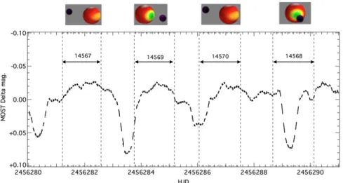
lists the start and stop HJD, phases, and exposure durations for the four individual observations. Figure 1 shows the time intervals of each observation superposed on the simultaneous MOST optical light curve ofδ Ori A (Pablo et al.2015). The
Chandra observations provide both MEG and HEG dispersed
first order spectra as well as the zeroth order image. Due to spacecraft power considerations as well as background count rate issues, it was necessary to use onlyfive ACIS CCD chips instead of six; thus, chip S5 was not used. This means that wavelengths longer than about 19 Å in the MEG plus-side dispersed spectrum and about 9.5 Å in the HEG plus-side dispersed spectrum are not available. Therefore, the strong OVIIline at 21 Å was only observed in the MEG-1 order. The
buildup of contaminants on the ACIS-S optical blockingfilters with time further degraded the long wavelength sensitivity for all first-order spectra. Each of the four observations experi-enced a large variation in focal plane temperature during the observation. While a temperature-dependent calibration is applied to each observation in standard data processing, the calibration is based on a single temperature measurement taken at the end of the observation. In particular, the focal plane temperature for portions of each observation exceeded the temperature at which the temperature-dependent effects of charge transfer inefficiency are calibrated (Grant et al.2006).
This could cause residual errors in the correction of pulse heights for those portions of the observations in the high-temperature regime.
Each ObsID was processed using the standard processing pipeline used in production of the Chandra Transmission Grating Data Archive and Catalog(Huenemoerder et al.2011).
Briefly, event filtering, event transformation, spectral extrac-tion, and response generation are done with standard Chandra Interactive Analysis of Observations software tools(Fruscione et al. 2006) as described in detail by Huenemoerder et al.
(2011). This pipeline produces standard X-ray events, spectra,
responses, effective areas, aspect histograms, and light curves. We used version 4.5.5 of the Chandra Calibration Database, along with CIAO version 4.5 and 4.6 in the analysis presented here. In order to examine variability, the data were also divided into ∼10 ks segments, and spectra, response files, effective areas, and light curves were generated for each segment. Analysis of the time-sliced data is presented in Nichols et al.(2015).
5. ANALYSIS OF THE X-RAY IMAGE
The δ Ori Aa1,2 inner binary is orbited by a more distant tertiary component(δ Ori Ab) at a current projected separation of 0″.3 with an orbital period of »346years (Tokovinin et al.2014). This separation is just below the spatial resolution
of Chandra, and thus Chandra imaging observations allow us to spatially examine the X-ray contribution from the Ab component. Figure2shows unbinned zeroth-order images from our four HETGS+ACIS observations, along with the expected location of Ab and the Aa pair at the times of the Chandra observations in 2012.
To constrain the X-ray contribution of δ Ori Ab, we
generated zeroth-order images for the four individual pointings
Table 2
New Chandra Observations ofδ Ori Aa+Ab
ObsID Start Start End End Midpoint Midpoint DT Exposure Roll
HJD Phase HJD Phase HJD Phase Days s degree
14567 2456281.21 396.604 2456282.58 396.843 2456281.90 396.724 1.37 114982 345.2 14569 2456283.76 397.049 2456285.18 397.297 2456284.47 397.173 1.42 119274 343.2 14570 2456286.06 397.450 2456287.52 397.705 2456286.79 397.578 1.46 122483 83.0 14568 2456288.67 397.905 2456290.12 398.159 2456289.39 398.032 1.45 121988 332.7
listed in Table2, using the Energy-Dependent Subpixel Event Repositioning24method to generate images with a pixel size of 0″.125. We generated images in 0.3−1 and 1−3 keV bands, but found no significant differences in any of the four observations when we compared the soft and hard band images. For each image, we then applied the CIAO tool SRCEXTENT to calculate the size and associated uncertainty of the photon-count source image or using the Mexican Hat Optimization algorithm.25
The results of the SRCEXTENT analysis are given in Table3. The derived major and minor axes of each image are equal and consistent with the Chandra point-spread function,
0. 3
~ . The peak of the image is consistent with the location of the Aa component, and is about a factor of two farther than the Ab component. We conclude that the peak positions of the zeroth-order images indicate that Aa is the primary X-ray source, with little or no contribution from Ab. Our analysis also suggests that the ObsID 14568 image may be slightly elongated, which may indicate a possible issue with the instrumental pointing or aspect reconstruction for this observation.
6. COMBINED SPECTRUM
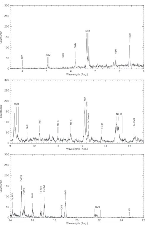
Figure 3 shows the co-added spectrum from the four
observations, with a total exposure of 479 ks. This represents the second longest exposure yet obtained on a massive star at wavelengths Å and a resolving power of8 lD >l 400. The strongest lines are OVIII, FeXVII, NeXI and NeX, MgXI and
MgXII, and SiXIII.
Figure 1. Timings of the Chandra observations along with the MOST light curve. The images above the plot show the orientations of δ Ori Aa1 and Aa2 near the midpoint of the observation according to the photometric and spectroscopic analysis of Pablo et al.(2015). In the images, the orbital angular momentum vector lies close to the plane of the paper and points to the top of the page.
Figure 2. Unbinned images from the four ObsIDs listed in Table2. ObsIDs, left to right: 14567, 14568, 14569, and 14570. The positions of Aa and Ab are shown by the full and dashed circles, respectively.
Table 3
SRCEXTENT Analysis Results
Band Major Axis Minor Axis PA Peak Dis-tance Aa Peak Dis-tance Ab ObsID keV arcsec arcsec degree arcsec arcsec 14567 0.3–1 0.34 0.33 83.3 0.19 0.40 1–3 0.32 0.28 83.8 0.19 0.42 14569 0.3–1 0.32 0.32 32.1 0.23 0.44 1–3 0.29 0.28 27.6 0.25 0.47 14570 0.3–1 0.32 0.32 136.9 0.09 0.35 1–3 0.26 0.22 48.3 0.08 0.34 14568 0.3–1 0.51 0.32 35.9 0.24 0.41 1–3 0.48 0.25 31.2 0.24 0.42 24 http://cxc.harvard.edu/ciao4.4/why/acissubpix.html 25 http://cxc.harvard.edu/ciao/ahelp/srcextent.html
6.1. Temperature Distribution
We modeled the combined spectrum with a combination of absorbed collisional ionization equilibrium models using the Interactive Spectral Interpretation System (ISIS; Houck & Denicola 2000). The model we applied includes two
low-temperature components seen through a common absorption component, plus a third hotter component with its own absorption component to account for any contribution from a hot colliding wind region embedded within the wind of the binary (see Section 7 below). In ISIS terminology, the mode we used was “(xaped(1)+xaped(2))*TBabs(3)+xaped(4)*TBabs(5),” where “xaped” represents emission from an optically thin plasma in collisional ionization equilibrium based on the ATOMDB atomic database version 2.0.2 (Smith & Brickhouse 2000; Foster
et al. 2012), and “TBabs” represents interstellar absorption
(Wilms et al.2000a). Solar abundances were assumed for both
the emission and absorption components.26 This model is an approximation to the actual temperature distribution and absorp-tion, but is the simplest one we found that adequately describes the observed grating spectrum. We allowed for velocity broad-ening of the emission lines, with turbulent velocity broadbroad-ening constrained to be less than roughly twice the maximum wind terminal velocity, 3000 km s−1. We allowed the line centroid velocities of the three emission components to vary, but found that overall the line centroids are unshifted in the combined
Figure 3. Combined MEG+HEG spectrum of δ Ori A, from 3.5 to 26 Å.
26
Shenar et al.(2015) show that N and Si are slightly sub-solar, but these differences are not significant for our analysis.
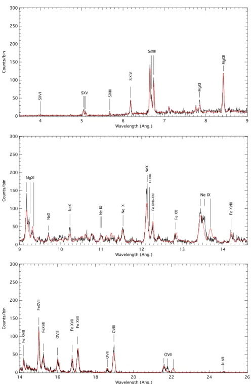
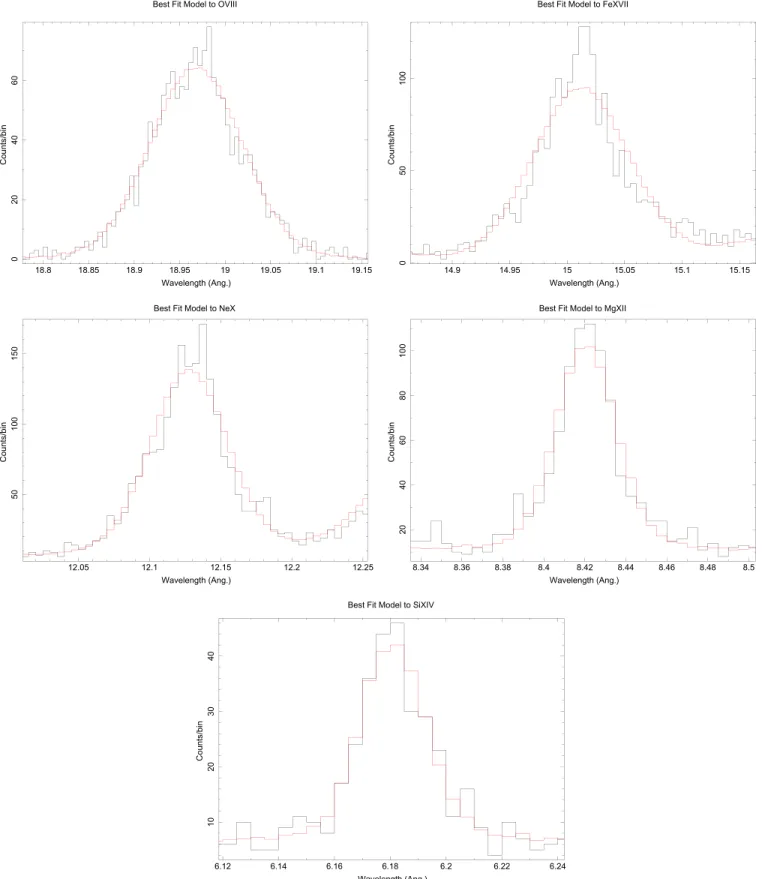
spectrum. Figure4compares the best-fit model to the data, while the model components are given in Table4. In this table, we also convert the derived turbulent velocities Vturb to equivalent line
half-widths at half maximum, using OVIII, NeXand MgXIIfor the
low-, medium-, and high-temperature components, respectively. The derived temperature distribution is similar to that found by Miller et al. (2002) in their study of the 2000 January
HETGS spectrum, and by Raassen & Pollock (2013) in their
analysis of an LETGS spectrum from 2007 November. In general, aside from the overall weakness of the forbidden lines compared to the model spectrum(which assumes a low-density plasma with no UV photoexcitation), the overall distribution of emission line strengths, and the continuum, are described
reasonably well by the model. We note, in reality, that this three-temperature model is a simplified representation of the actual emission measure distribution with temperature. This multitemperature model mainly provides us with an adequate approximation of the local (pseudo-) continuum in order to improve linefitting and modeling.
6.2. Emission Lines
The observed X-ray emission lines in ourδ Ori A spectrum provide important diagnostic information about the phase-averaged state of the hot gas within the wind of the system, and, as we show below, this is dominated by the shocked gas
Figure 4. Combined MEG+HEG spectrum of δ Ori A (in black) with the three-component fit (shown in red) given in Table4. The model spectra, which assume low density and do not include effects of UV photoexcitation, generally overestimate the strength of the forbidden lines and underestimate the strengths of the intercombination lines, especially at longer wavelengths, most notably at OVII.
embedded within the wind ofδ Ori Aa1, with little contribution (if any) from gas heated by the shock produced by the collision of the wind fromδ Ori Aa1 with the wind or photosphere of δ Ori Aa2. The analysis of the set of emission lines depends on choice of line profile, continuum level, and accounting for line blends.
6.2.1. Gaussian Modeling
To better account for blends and uncertainties in the continuum level, we performed a Gaussian fit to the strong lines, allowingflux, line width, and centroid velocity to vary. These fits, shown in Figure 5, were done using the three-temperaturefit given in Section6.1to define the continuum and amount of line blending. We set the abundance of the element to be measured to zero, with the abundances of other elements set to solar and other parameters (temperature, absorptions) fixed at the values given in Section4. This procedure is useful to account for line blends, in particular, for the NeX line at
12.132 Å, which is blended with an FeXVII line at 12.124 Å.
We assumed simple Gaussian line profiles for the line to be fit, andfit for both the Ly 1a and Ly 2a lines, with line widths and velocities fixed for both components, and the intensity ratio of the Ly 2a to the Ly 1a line set to the emissivity ratio at the temperature of peak emissivity. We used the Cash statistic and ISIS (Houck & Denicola 2000) to perform the fits,
simulta-neouslyfitting the HEG and MEG ±1 order spectrum from all four observations simultaneously. Table 5 shows the result of fits of the H-like Lyα lines, plus the strong FeXVII line at
15.014 Å. In general, the Gaussian fits are poor (the reduced Cash statistic>1.5) except for the weak SiXIVline, though the
asymmetries in the bright lines are not very strong. All of the line centroids are near zero velocity, though the NeX line is
blueshifted at about the 2σ level.
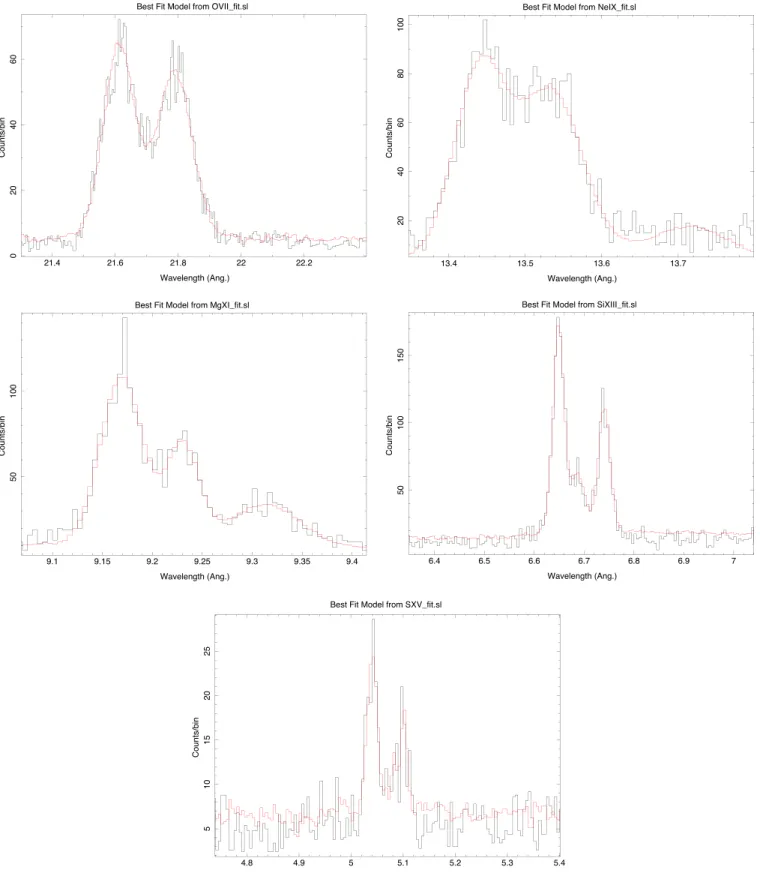
We also measured the forbidden (z), intercombination (x+y), and resonance components (w) above continuum for each of the helium-like ions(OVII, MgX, NeIX, and SiXIII) by
Gaussian fitting. As before, we used the three-temperature fit given in Section6.1to define the local continuum near the line region. Although the individual intercombination components (x+y) are unresolved in the HETGS spectra for all of the He-like ions, we included a Gaussian line for the x and y lines, but restricted the centroid velocity and line widths to be the same for both the x and y components. Because the forbidden, intercombination and resonance lines can have different spatial distributions throughout the wind, we allowed the widths, centroids, and line fluxes of these lines to vary individually. The forbidden component of the OVII line is weak, and, in
addition, this line was only observed in the MEG-1 spectrum arm because ACIS-S chip S5 was turned off due to spacecraft power constraints. To increase signal to noise for the OVII
forbidden line, and for the weak SiXIII and SXV triplets, we
included data from the 2001 HETG and 2008 LETG observations when fitting. Figure 6 shows the fits of the He-like lines, and Table6shows the results of this three-Gaussian componentfitting, while Table7shows the R=z x( +y)and G=(x+ +y z w) ratios.
Figure 7 shows the dependence of the half width at half maximum of the Gaussian fit versus the excitation energy of the upper level of the transition. The linear correlation coefficient for the H-like half-widths is −0.89, indicating a strong anti-correlation between line half-width and excitation energy. For the He-like lines, the linear correlation coefficient is−0.81, also indicating a strong anti-correlation of line half-widths and excitation energy. Thus the line half-widths are anti-correlated with the upper energy level, in that the line width decreases with excitation energy. This anti-correlation shows that the more highly excited lines form at lower velocities, and thus closer to the stellar surface of the primary, indicating that the higher-temperature X-ray emission emerges from deeper regions in the wind than the cooler emission.
In Figure7, the OVIIline width seems lower compared to the
trend defined by the more highly excited ions. Excluding the OVII line, a linear fit to the remaining He-like lines yields a
linear correlation coefficient of −0.87, indicating a stronger anti-correlation, and also results in a steeper linear slope. This linearfit predicts that the OVIIline should have a half-width of
918 eV, a factor of 1.2 larger than observed. We caution that, unlike the other lines, the OVIIline was only observed in one
grating order since ACIS-S chip 5 was switched off during these observations.
As a crude approximation, if we assume that the X-ray emitting material resides in a thin spherical shell at radius r aroundδ Ori Aa1, then the line profile will extend from V r- ( ) to +V r( ) 1-(RAa1 r)2, where RAa1 is the radius of δ Ori Aa1, and V r( )=V¥,Aa1(1-RAa1 r)b, the standard velocity law for radiatively driven winds. The inverse correlation of the line widths with excitation energy suggests that the hotter X-ray emitting gas is formed over a smaller volume in the wind acceleration zone closer to the star, where wind radial velocity differentials are larger and where higher temperature shocks can be generated; cooler ions can be maintained farther out in the wind where the acceleration(and thus the velocity differential) is smaller. A similar conclusion was reached by Hervé et al. (2013) in their analysis of ζ
Puppis.
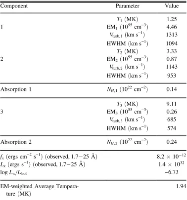
Table 4
Best-fit to the Combined HETGS Spectrum. The Adopted Model is (APED1+APED2)*NH,1+APED3*NH,2
Component Parameter Value T1(MK) 1.25 1 EM1(1055cm−3) 4.46 Vturb,1(km s−1) 1313 HWHM(km s−1) 1094 T2(MK) 3.33 2 EM2(1055cm−3) 0.87 Vturb,2(km s−1) 1143 HWHM(km s−1) 953 Absorption 1 NH,1(1022cm−2) 0.14 T3(MK) 9.11 3 EM3(1055cm−3) 0.26 Vturb,3(km s−1) 685 HWHM(km s−1) 574 Absorption 2 NH,2(1022cm−2) 0.24 fx(ergs cm−2s−1) (observed, 1.7 25- Å) 8.2´10-12 Lx(ergs s−1) (observed, 1.7 25- Å) 1.4´1032 L L log x bol −6.73
EM-weighted Average Tempera-ture(MK)
Figure 5. Top to bottom, left to right: OVIII, FeXVII, NeX, MgXII, and SiXIV. The lines are plotted in the velocity range of−3000 to +3000 km s−1. The best-fit Gaussian profile, and the continuum derived from the model parameters given in Table4is shown in red. Note that while most of the Lyα lines are adequately described by a symmetric Gaussian, the FeXVIIand NeXlines are not as wellfit by simple Gaussian profiles as the other lines. This may be due to the effects of non-uniform X-ray line opacity, as discussed in Section6.2.2.
6.2.2. Effects of X-Ray Line Opacity
The possibility that strong resonance line photons might be scattered out of the line of sight has significant implications on our physical understanding of the X-ray emission from hot stars, especially in the interpretation of mass-loss rates derived from X-ray line profiles and abundances derived from X-ray line ratios. Resonance scattering may be important for lines with high oscillator strengths and could, in principle, change the line shape or intensity ratios, though recent analysis by Bernitt et al.(2012) suggested that our poor knowledge of the
underlying atomic physics may play the dominant role in accounting for discrepancies in line intensities. Miller et al. (2002) focussed on the FeXVII lines at 15.014 and 15.261 Å,
which have oscillator strengths of 2.49 and 0.64, respectively. Resonance scattering might significantly affect the 15.014 Å emission line, which is one of the strongest lines in theδ Ori A X-ray spectrum, while scattering should be unimportant for the weak 15.261 Å line. Miller et al. (2002) found that the
observed ratio of these two lines, as derived from their Chandra grating spectrum, was I15.01 15.26I =2.41.3, nominally (though not significantly) below the optically thin limit I15.01 15.26I =3.5 derived from the Smith & Brickhouse
(2000) version of the Astrophysical Plasma Emission
Code (APEC).
We re-examined this issue for these two FeXVIIlines using
our deeper spectrum and a slightly different technique. We isolated the FeXVIIline region in the combined spectrum andfit
this restricted region with an APEC-derived model, with abundances fixed at solar, including line broadening. We first fit the FeXVIIline at 15.261 Å, ignoring the region around the
stronger 15.014 Å line. We then included the 15.014 Å line region and compared the predicted strength of the model 15.014 Å line to the observed line. This technique, in which we use a full thermal model to fit the spectra rather than a simple comparison of line intensities, has the benefit that line blends in the region will be more properly taken into account. We found that the model based on the bestfit to the 15.261 Å line greatly overpredicted the strength of the 15.014 Å line, and can be ruled out at high confidence (c =n2 3.57, restricted
to the 14.90–15.14 Å region; excluding this region,
0.72
2
c =n ). This may be an indication of the effect of
resonance scattering on the 15.014 Å FeXVII line. Since it
appears that the 15.014 Å line is a bit narrower than the 15.261 Å line, we also re-did thefit, allowing the width of the 15.014 Å line to differ from that of the 15.261 Å line. We then re-fit only the 15.014 Å line, allowing the line broadening to vary and also allowing the normalization to vary. Figure 8
shows the resultingfit. The best-fit HWHMs for the 15.014 and 15.261 Å lines are 1275-+26848 and 1496-+113109km s−1, respectively,
while the model normalizations are 0.0024-+0.0010.0001 and
0.0030 0.001 0.001
-+ for the 15.014 and 15.261 Å lines, respectively.
This analysis also shows the 15.014 Å line is significantly weaker than expected compared to the 15.261 Å line. This again may indicate that resonance scattering plays a role in determining the line profile shape and line strength, at least for the FeXVIIline, though uncertainties in the atomic models and
in our definition of the temperature distribution for δ Ori A may play a significant role in altering the intensity ratios for these lines.
To further investigate the importance of resonance scatter-ing, we also considered the NeX lines at 10.239 Å and at
12.132 Å, which have oscillator strengths of 0.052 and 0.28, respectively. These lines complement the FeXVIIanalysis since
for NeXthe stronger line appears at longer wavelengths; this
means that any effects of differential absorption that might affect the FeXVIIline analysis would have the opposite effect
on the NeXlines. We again fit the NeX10.239 Å line with a
single temperature APEC model, butfixed the temperature to the temperature of maximum emissivity of the NeXlines, i.e.,
T=6.3´106K. We then compared the model that bestfits
the NeX10.239 Å line to the NeX12.132 Å line. Note that the
NeX12.132 Å line is blended with the FeXXIline at 12.285 Å
(which has a temperature of maximum emissivity of 12.6´106K, about twice that of the NeX line), so we
restricted the NeX 12.132 Å fitting region to the interval
12.0–12.22 Å. We again find that the model, which provides a good fit to the weaker line (c =n2 0.79), overpredicts the strength of the stronger line (c =n2 8.63), again a possible indication that resonance scattering is important in determining theflux of the strong line.
7. THE INFLUENCE OF COLLIDING WINDS ON THE EMBEDDED X-RAY EMISSION
Colliding winds can have important observable effects in our analysis of the X-ray emission fromδ Ori Aa in two ways. The collision of the primary wind with the surface or wind of the secondary could produce hot shocked gas which might contaminate the X-ray emission from the embedded wind shocks in the primaryʼs unperturbed wind. In addition, the colliding wind“bow shock” around the weaker-wind second-ary produces a low-density cavity in the primsecond-ary wind, and this cavity, dominated by the weak wind ofδ Ori Aa2, should show little emission from embedded wind shocks.
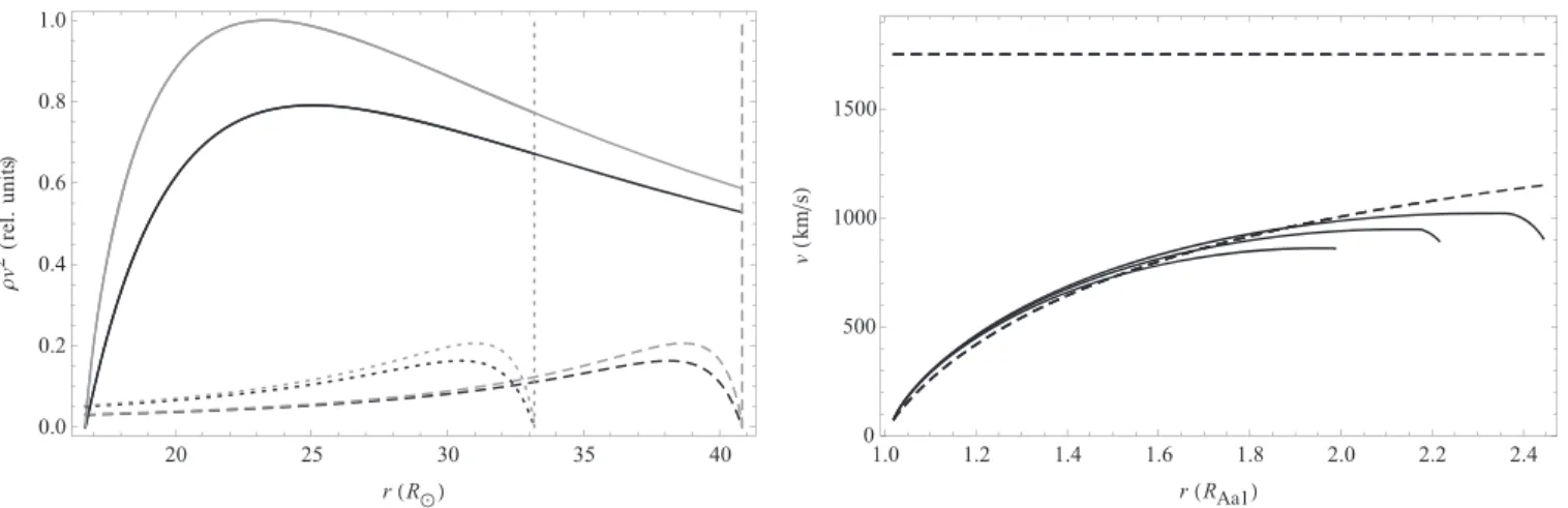
Along the line between the stars, the stellar winds will collide at the point at which their ram pressures vr ^2 are equal
(e.g., Stevens et al.1992). Using the stellar, wind, and orbital
parameters in Table1, Figure 9 shows the ram pressures for Aa1 (solid) and Aa2 (dashed: apastron, dotted: periastron) assuming that the wind from each star follows the standardβ velocity law, V r( )=v¥(1 -R r)b, where V r( ) is the wind radial velocity at a distance r from the star, R is the stellar radius, and we assume thatb =0.8or 1.0. The ram pressure of Aa1ʼs wind is greater than that of Aa2 throughout the orbit, so the wind from Aa1 should directly impact Aa2ʼs surface, in this simple analysis.
A more thorough treatment includes the effects of Aa2ʼs radiation on the wind of Aa1 (and vice versa). These effects include “radiative inhibition” (Stevens & Pollock 1994) in
which Aa1ʼs wind acceleration along the line between the stars is reduced by Aa2ʼs radiative force acting in opposition to the
Table 5
Gaussian Fits to the H-like Lines, Plus FeXVII
λ Flux V HWHM Ion Å (10−5ph. s−1cm−2) (km s−1) (km s−1) OVIII 18.967 219-+109 -9-+3337 918-+2938 FeXVII 15.014 76-+34 -24-+3542 971-+2753 NeX 12.132 10-+11 -102-+4250 726-+5848 MgXII 8.419 1-+00 -12-+5533 547-+6158 SiXIV 6.180 0.35-+0.050.05 -49-+13445 544-+124116
wind flow, and “sudden radiative braking” (Owocki & Gayley 1995; Gayley et al.1997), where Aa1ʼs strong wind,
which would otherwise impact the surface of Aa2, is suddenly decelerated by Aa2ʼs radiation just above the surface of Aa2. To estimate the magnitude of these effects, we solve the 1D
equation of motion along the line of centers, accounting for both starʼs radiative forces via the standard Castor, Abbott, and Klein (CAK) line forces (Castor et al. 1975), including the
finite disk correction factor (Friend & Abbott1986; Pauldrach et al. 1986) and gravitational acceleration. We determine the Figure 6. Top to bottom, left to right: O VII; Ne IX; Mg XI; Si XIII; S XV. The best fit, using a model of four Gaussian lines (w, x, y, and z components) and the continuum derived from the model parameters given in Table4, is shown in red.
CAK parameters Q¯ and α (Gayley1995) to yield the desired
mass-loss rates and terminal speeds for each star by using the standard reduction in mass-loss rate from the finite disk correction factor, i.e., M˙fd=M˙CAK (1+a)(1+a). We numeri-cally integrate the equation of motion to distances far from the star to yield the terminal velocity. Then we repeat the process including the radiation and gravity of both stars to determine the speed of each wind along the line between the stars.
Figure 9 shows the equation-of-motion solution for the primary wind. The initial velocity corresponds to a b =0.8 law, but radiative inhibition causes the wind (solid) to accelerate less compared to the unmodified β-law (dashed). In addition, the primary wind velocity does begin to decrease from radiative braking. However, Star Aa2ʼs surface is located at the end of each line, so that the primary wind does not completely stop before it impacts the secondary surface. This indicates that the wind from star Aa1 should still impact the surface of Aa2, even when the influence of the radiation field of star Aa2 is taken into account. Furthermore, due to the strong radiation of Aa1, the wind of Aa2 does not accelerate off the surface of the star toward Aa1, further suggesting that Aa1ʼs wind will directly impact Aa2ʼs surface.
We used a 3D smoothed particle hydrodynamics(SPH) code developed by Benz & Buchler(1990) and Bate et al. (1995) to
model the effects of the wind–wind collision on the extended system wind. Okazaki et al.(2008) was first to apply this code
to a colliding-wind system, and Russell (2013) and Madura
et al.(2013) describe the current capabilities of the code, which
we briefly state here. The stars are represented as two point masses, and throughout their orbit they inject SPH particles into the simulation volume to represent their stellar winds. The SPH particles are accelerated away from their respective stars according to aβ =1 law (absent from any influence from the companionʼs radiation) by invoking a radiative force with a radially varying opacityk( )r , i.e., grad =k( )r F c, where F is the stellarflux. We take effects of the occultation of one starʼs radiation by the other star into account. Radiative inhibition is included in the code(within the context of the radially varying opacity method), but radiative braking is not since it requires the full CAK solution for the wind driving, which is not yet included in the SPH code. Radiative cooling is implemented
via the Exact Integration Scheme (Townsend2009), and the
abundances of both winds are assumed to be solar (Asplund et al.2009).
The importance of radiative cooling of the shocked material is determined by the parameter c =d v12 84 M˙-7 (Stevens
et al. 1992), where d12 is the distance to the shock in
1012cm, v8is the preshock velocity in 10 8
cm s−1, and M˙-7 is
the mass-loss rate in 10−7Myr−1. c >1 indicates adiabatic
expansion is more important, while c <1 indicates that the shocked gas will cool radiatively. For theβ =1 law, χ ranges from 0.5c1.3 between periastron to apastron, so the shocked gas should cool through a combination of adiabatic expansion and radiation.
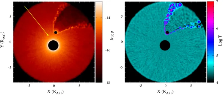
Figure10shows the density and temperature structure of the interacting winds in the orbital plane using the parameters in Table 1. The primary wind impacts the secondary star as expected from the analytical treatment above, where it shocks with newly injected secondary SPH particles. If this interaction leads to SPH particles, either belonging to Aa1 or Aa2, going within the boundary of the secondary star, these particles are accreted, i.e., removed from the simulation. The temperature plot of Figure 10 shows that this leads to hot, shocked gas around Aa2, but this must be deemed approximate since the code does not force the Aa1 particles to accrete at the sound speed, which would increase the shock temperature, nor does it include any reflection of Aa1ʼs radiation off of the surface of Aa2, which would decrease the shock temperature. The half-opening angle is~ , so30 ~8% of the solid angle of Aa1ʼs wind is evacuated by Aa2 and its wind.
To determine the X-rayflux from the wind–wind/wind–star collision, we solve the formal solution to radiative transfer along a grid of rays through the SPH simulation volume, for which we use the SPH visualization program Splash (Price 2007) as our basis. The emissivity is from the APEC
model (Smith et al. 2001) obtained from XSPEC
(Arnaud 1996), the circumstellar material absorbs according
to the windtabs model (Leutenegger et al. 2010), and the
interstellar absorption is from TBabs (Wilms et al. 2000b).
The radiative transfer calculation is performed at 170 energies logarithmically spaced from 0.2 to 10 keV(100 per dex), and generates surface brightness maps for each energy. These are then summed to determine the model spectrum, and finally folded through X-ray telescope response functions to directly compare with observations. The overall contamination level of wind–wind/wind–star collision X-rays is <10% of the Chandra zeroth-order ACIS-S observation, so the influence of emission from shocked gas along the wind–wind boundary is not very significant, though contamination may be larger in some regions of the spectrum, depending on the emission-measure temperature distribution of the colliding-wind X-rays compared to that of the X-rays arising from embedded wind
Table 6
Gaussian Fits to the He-like Lines
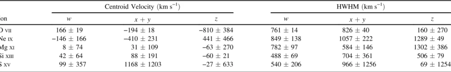
Centroid Velocity(km s−1) HWHM(km s−1) Ion w x+y z w x+y z OVII 166± 19 −194 ± 18 −810 ± 384 761± 14 826± 40 160± 270 NeIX −146 ± 166 −410 ± 231 441± 466 849± 138 1057± 222 1289± 49 MgXI 8± 74 31± 109 −63 ± 270 782± 97 584± 146 1302± 386 SiXIII 42± 64 88± 191 −60 ± 21 488± 69 704± 361 506± 79 SXV 99± 357 1168± 1203 −27 ± 633 540± 206 966± 1256 69± 1254 Table 7 R and G Ratios Ion R=z x( +y) G=(x+ +y z w) OVII 0.04± 0.01 0.94± 0.26 NeIX 0.27± 0.10 1.44± 0.65 MgXI 0.96± 0.36 0.95± 0.37 SiXIII 1.77± 0.18 0.90± 0.12 SXV 3.88± 2.86 0.72± 0.74
Figure 7. Half-widths of the H-like Lyα lines (km s−1) and the He-like resonance lines vs. excitation energy (eV) of the upper level of the transition. The full and
dashed lines represent the best linearfit to the HWHMs from the H-like lines, and the He-like lines (excluding the OVIIwidth), respectively.
Figure 8. Left: APEC-based modeling of the FeXVII15.014 vs. 15.261 Å lines. Wefirst fit the 15.261 Å line by itself. The thick histogram compares that model to the observed spectrum in the 14.5–15.6 Å range. This shows that the model that fits the 15.26 Å line overpredicts the strength of the 15.0 Å line. The vertical lines from the continuum to the X axis at 14.9 and 15.14 Å show the adopted wavelength range of the 15.014 Å FeXVIIline. Right: APEC modelfit to the NeX10.24 Å compared to the NeX12.134 Å line. The model(shown by the thick histogram) that fits the weaker 10.24 Å line overpredicts the strength of the stronger 12.134 Å line.
Figure 9. Left: Ram pressure of Aa1 (solid) and Aa2 at apastron (dashed) and periastron (dotted). The black lines show a β = 1 law, while the gray lines show a β = 0.8 law. The gray vertical lines represent the location of Aa2ʼs surface for these two phases. Right: 1D solution to the equation of motion of the primary wind along the line between the stars(solid) at three different separations—apastron (top), semimajor axis (middle), and periastron (bottom). For comparison, the dashed curve shows aβ = 0.8 law, and the dashed line shows terminal velocity.
shocks. We caution, however, that the model X-ray flux is dependent on the boundary condition imposed at the surface of Aa2, and so imposing a condition where the incoming wind from star Aa1 shocks more strongly (weakly) will increase (decrease) the amount of X-ray emission from the wind–star collision.
8. CONCLUSIONS
Delta Ori Aa is an X-ray bright, nearby, eclipsing binary and so offers the potential to directly probe the X-ray emitting gas distribution in the primary starʼs wind as the secondary star revolves through the primaryʼs wind. Our Chandra program was designed to obtain high signal-to-noise and high spectral resolution spectrometry of this system throughout an entire orbit. In this paper, we have sought to characterize the overall spectrum at its highest signal-to-noise ratio by combining all of the Chandra spectra and examining temperature distributions and line parameters. Our main results are presented below.
1. Our analysis of the Chandra image shows that the emission is mostly dominated by δ Ori Aa, with little detectable emission fromδ Ori Ab.
2. The temperature distribution of the X-ray emitting gas can be characterized by three dominant temperatures, which agrees fairly well with the temperature distribu-tions derived by the earlier analysis of Miller et al.(2002)
and Raassen & Pollock(2013).
3. The strong lines are generally symmetric, and Gaussian profiles provide a reasonable representation of the profile shape, though in most cases, and especially for the NeX
and FeXVII, there are significant deviations from Gaussian
symmetry.
4. The line widths determined by Gaussian modeling shows that half-widths are typically0.3 0.5- ´V¥, where V¥is
the terminal velocity of the wind of δ Ori Aa1. These values are generally larger than the line widths measured by Miller et al. (2002), though it is unclear whether this
represents a real change in the line profile or if there is a calibration issue in the analysis of the earlier data set, which was obtained at an anomalously high focal plane temperature.
5. We find a strong anti-correlation between the widths of the H-like and He-like transitions and the excitation energy. This indicates that the lower-energy transitions occur in a region with larger velocities. Assuming a standard wind acceleration law, this correlation probably indicates that the lower-energy lines emerge from further out in the wind.
6. Analysis of strong and weak transitions of FeXVII and
NeXindicates that resonance scattering may be important
in determining theflux and/or shape of the stronger line. This agrees with the analysis of the FeXVIIline by Miller
et al. (2002) but at higher significance. We caution that
some of these differences in the observed to predicted line ratios may be influenced by an inaccurate temperature distribution and/or uncertainties in the atomic physics. It is also interesting to note that these two lines also have the most non-Gaussian profiles, as shown in Figure 5, perhaps indicative that some line photons have been scattered out of the line of sight.
The spectrum combined from the four individual Chandra-HETGS observations represents a very high signal-to-noise
view of the emission from δ Ori Aa. However, these
observations were obtained at a variety of orbital phases, so that the combined spectrum is a phase-averaged view of the overall X-ray emission fromδ Ori Aa. In a companion paper (Nichols et al., 2014, Paper II), we look for the effects of phase- and time-dependent changes in the continuum and line spectrum.
We thank the MOST team for the award of observing time for δ Ori A. We also thank our anonymous referee, whose comments significantly improved this paper. M.F.C. thanks
5 0 -5 5 0 -5 -18 -16 -14 6 7 5 4 -5 0 5 -5 0 5 Y ( RAa1 ) X (RAa1) X (RAa1) log ρ Log T
Figure 10. Density (left) and temperature (right) structure in the orbital plane from the SPH simulation of δ Ori Aa1 (larger star) and δ Ori Aa2 (smaller star). The arrow shows the orientation of the line of sight. The system is pictured at phasef =0.87. The collision of the wind fromδ Ori Aa1 against δ Ori Aa2 produces a low-density cavity in the wind ofδ Ori Aa1, where the emission from embedded wind shocks is reduced. The collision also produces a layer of hot shocked gas at the boundary of the cavity which produces< % of the emission from the wind shocks embedded in the unperturbed wind from10 δ Ori Aa1. In the temperature plot on the right, the hot gas from embedded wind shocks in the winds fromδ Ori Aa1 and δ Ori Aa2 is ignored, to emphasize the hot gas along the wind collision boundary.
John Houck and Michael Nowak for many helpful discussions concerning data analysis with ISIS. Support for this work was provided by the National Aeronautics and Space Administra-tion through Chandra Award Number 14015A and GO3-14015E issued by the Chandra X-ray Observatory Center, which is operated by the Smithsonian Astrophysical Observa-tory for and on behalf of the National Aeronautics Space Administration under contract NAS8-03060. M.F.C., J.S.N., W.L.W., C.M.P.R., and K.H. gratefully acknowledge this support. M.F.C. acknowledges support from NASA under cooperative agreement number NNG06EO90A. N.R.E. is grateful for support from the Chandra X-ray Center NASA Contract NAS8-03060. C.M.P.R. is supported by an appoint-ment to the NASA Postdoctoral Program at the Goddard Space Flight Center, administered by Oak Ridge Associated Uni-versities through a contract with NASA. T.S. is grateful for financial support from the Leibniz Graduate School for Quantitative Spectroscopy in Astrophysics, a joint project of the Leibniz Institute for Astrophysics Potsdam (AIP) and the institute of Physics and Astronomy of the University of Potsdam. Y.N. acknowledges support from the Fonds National de la Recherche Scientifique (Belgium), the Communauté Française de Belgique, the PRODEX XMM and Integral contracts, and the “Action de Recherche Concertée” (CFWB-Académie Wallonie Europe). N.D.R. gratefully acknowledges his CRAQ(Centre de Recherche en Astrophysique du Québec) fellowship. A.F.J.M. is grateful for financial support from NSERC(Canada) and FRQNT (Quebec). J.L.H. acknowledges support from NASA award NNX13AF40G and NSF award
AST-0807477. This research has made use of NASAʼs
Astrophysics Data System. This research has made use of data and/or software provided by the High Energy Astrophysics
Science Archive Research Center (HEASARC), which is a
service of the Astrophysics Science Division at NASA/GSFC and the High Energy Astrophysics Division of the Smithsonian Astrophysical Observatory. This research also made use of the Chandra Transmission Grating Catalog and archive (http:// tgcat.mit.edu). The SPH simulations presented in this paper
made use of the resources provided by the NASA High-End
Computing (HEC) Program through the NASA Advanced
Supercomputing(NAS) Division at Ames Research Center. REFERENCES
Arnaud, K. A. 1996, in ASP Conf. Ser. Vol. 101, Astronomical Data Analysis Software and Systems V, ed. G. H. Jacoby & J. Barnes(San Francisco, CA: ASP), 17
Asplund, M., Grevesse, N., Sauval, A. J., & Scott, P. 2009, ARA&A,
47, 481
Bate, M. R., Bonnell, I. A., & Price, N. M. 1995, MNRAS,277, 362
Benz, W. 1990, in Numerical Modelling of Nonlinear Stellar Pulsations Problems and Prospects, ed. J. R. Buchler(Dordrecht: Kluwer), 269 Berghoefer, T. W., Schmitt, J. H. M. M., Danner, R., & Cassinelli, J. P. 1997,
A&A,322, 167
Bernitt, S., Brown, G. V., Rudolph, J. K., et al. 2012,Natur,492, 225
Brinkman, A. C., van Rooijen, J. J., Bleeker, J. A. M., et al. 1987, ApL&C,
26, 73
Caballero, J. A., & Solano, E. 2008,A&A,485, 931
Canizares, C. R., Davis, J. E., Dewey, D., et al. 2005,PASP,117, 1144
Cantiello, M., Langer, N., Brott, I., et al. 2009,A&A,499, 279
Cassinelli, J. P., & Swank, J. H. 1983,ApJ,271, 681
Castor, J. I., Abbott, D. C., & Klein, R. I. 1975,ApJ,195, 157
Chlebowski, T., Harnden, F. R., Jr., & Sciortino, S. 1989,ApJ,341, 427
Cohen, D. H., Wollman, E. E., Leutenegger, M. A., et al. 2014, arXiv:1401.7995
Corcoran, M. F., Waldron, W. L., Macfarlane, J. J., et al. 1994,ApJL,436, L95
Fisher, P. C., & Meyerott, A. J. 1964,ApJ,139, 123
Foster, A. R., Ji, L., Smith, R. K., & Brickhouse, N. S. 2012,ApJ,756, 128
Friend, D. B., & Abbott, D. C. 1986,ApJ,311, 701
Fruscione, A., McDowell, J. C., Allen, G. E., et al. 2006,Proc. SPIE,6270, 1
Gayley, K. G. 1995,ApJ,454, 410
Gayley, K. G., Owocki, S. P., & Cranmer, S. R. 1997,ApJ,475, 786
Gräfener, G., Koesterke, L., & Hamann, W.-R. 2002,A&A,387, 244
Grant, C. E., Bautz, M. W., Kissel, S. E., LaMarr, B., & Prigozhin, G. Y. 2006, Proc. SPIE,6276, 1
Haberl, F., & White, N. E. 1993, A&A,280, 519
Hamann, W.-R., & Gräfener, G. 2003,A&A,410, 993
Harmanec, P., Mayer, P., & Slechta, M. 2013, in Proc. Massive Stars: from Alpha to Omega
Hartmann, J. 1904,ApJ,19, 268
Harvin, J. A., Gies, D. R., Bagnuolo, W. G., Jr., Penny, L. R., & Thaller, M. L. 2002,ApJ,565, 1216
Hervé, A., Rauw, G., & Nazé, Y. 2013,A&A,551, A83
Houck, J. C., & Denicola, L. A. 2000, in ASP Conf. Ser. 216, Astronomical Data Analysis Software and Systems IX, ed. N. Manset, C. Veillet & D. Crabtree(San Francisco, CA: ASP), 591
Huenemoerder, D. P., Mitschang, A., Dewey, D., et al. 2011, AJ,141, 129
Koch, R. H., & Hrivnak, B. J. 1981,ApJ,248, 249
Kudritzki, R., & Puls, J. 2000,ARA&A,38, 613
Leutenegger, M. A., Cohen, D. H., Zsargó, J., et al. 2010,ApJ,719, 1767
Leutenegger, M. A., Paerels, F. B. S., Kahn, S. M., & Cohen, D. H. 2006,ApJ, 650, 1096
Long, K. S., & White, R. L. 1980,ApJL,239, L65
Lucy, L. B., & White, R. L. 1980,ApJ,241, 300
Madura, T. I., Gull, T. R., Okazaki, A. T., et al. 2013,MNRAS,436, 3820
Mayer, P., Harmanec, P., Wolf, M., Božić, H., & Šlechta, M. 2010,A&A,
520, A89
Miller, N. A., Cassinelli, J. P., Waldron, W. L., MacFarlane, J. J., & Cohen, D. H. 2002,ApJ,577, 951
Nichols, J. S., Huenemoerder, D. P., Corcoran, M. F., et al. 2015, ApJ, 809, 133
Okazaki, A. T., Owocki, S. P., Russell, C. M. P., & Corcoran, M. F. 2008,
MNRAS,388, L39
Oskinova, L. M., Feldmeier, A., & Hamann, W.-R. 2006, MNRAS, 372, 313
Owocki, S. P., & Cohen, D. H. 2006,ApJ,648, 565
Owocki, S. P., Cranmer, S. R., & Gayley, K. G. 1996,ApJL,472, L115
Owocki, S. P., & Gayley, K. G. 1995,ApJL,454, L145
Pallavicini, R., Golub, L., Rosner, R., et al. 1981,ApJ,248, 279
Pauldrach, A., Puls, J., & Kudritzki, R. P. 1986, A&A,164, 86
Pablo, H., Richardson, N. D., Moffat, A. F. J., et al. 2015, ApJ, 809, 134 Price, D. J. 2007,PASA,24, 159
Raassen, A. J. J., & Pollock, A. M. T. 2013,A&A,550, A55
Richardson, N. D., Moffat, A. F. J., Gull, T. R., et al. 2015, arXiv:1506.05530
Russell, C. M. P. 2013, PhD thesis, Univ. Delaware
Shenar, T., Oskinova, L., Hamann, W.-R., et al. 2015, ApJ, 809, 135 Smith, R. K., & Brickhouse, N. S. 2000, in Revista Mexicana de Astronomia y
Astrofisica Conf. Ser. 9, Astrophysical Plasmas: codes, Models, and Observations, ed. S. J. Arthur, N. S. Brickhouse & J. Franco, 134 Smith, R. K., Brickhouse, N. S., Liedahl, D. A., & Raymond, J. C. 2001,ApJL,
556, L91
Snow, T. P., Jr., Cash, W., & Grady, C. A. 1981,ApJL,244, L19
Sota, A., Maõz Apellaniz, J., Morrell, N. I., et al. 2014,ApJS,211, 10
Stebbins, J. 1915,ApJ,42, 133
Stevens, I. R., Blondin, J. M., & Pollock, A. M. T. 1992,ApJ,386, 265
Stevens, I. R., & Pollock, A. M. T. 1994,MNRAS,269, 226
Tokovinin, A., Mason, B. D., & Hartkopf, W. I. 2014,AJ,147, 123
Townsend, R. H. D. 2009,ApJS,181, 391
Walborn, N. R., Nichols, J. S., & Waldron, W. L. 2009,ApJ,703, 633
Waldron, W. L., & Cassinelli, J. P. 2001,ApJL,548, L45
Waldron, W. L., & Cassinelli, J. P. 2007,ApJ,668, 456
Walker, G., Matthews, J., Kuschnig, R., et al. 2003,PASP,115, 1023
Wilms, J., Allen, A., & McCray, R. 2000a,ApJ,542, 914