Cost prediction via quantitative analysis of complexity in U.S. Navy shipbuilding

(1)

COST PREDICTION VIA QUANTITATIVE ANALYSIS OF COMPLEXITY IN U.S. NAVY SHIPBUILDING

by

Aaron T. Dobson

B.S., Aerospace Engineering, United States Naval Academy Submitted to the Department of Mechanical Engineering and Engineering

Division in Partial Fulfillment of the Requirements for the Degrees Naval Engineer

and

Master of Science in Engineering and Management at the

Massachusetts Institute of Technology June 2014

The author hereby grants to MIT permission to reproduce and to distribute publicly paper and electronic copies of this thesis document

in whole or in part in any medium now known or hereafter created.

Signature redacted

Systems of ASsACHUSEMTS INTJfTE OF TECHNOLOGY

JUN 2

6

20 LIBRARIES

Signature of A uthor:... ... Department of Mechanical Engineering and S stem Design and Management

Signature redacted

May

9t

2014

Certified by:... ... - ... Olivier L. de Weck Professor of Aeronautics and Astg ics and Engineering Systems

Signature redacted-

Thesis Supervisor C ertified b y : ... ...

Eric S. Rebentisch RDsearch Associate, Sociotechnical Systems Research Center

-Signature

redacted.

Thesis Supervisor

Certifiede

beac:d

Accepted by:...

...

ar xas

Professor of the Pract e ard i ng

Signature redacted

es S S isor

... . . . ...

atrick Hale ZD7rector, System Design and Management Fellows Program

Signature

redacted

Engineering Systems Division

... David E. Hardt Chairman, Department Committee on Graduate Studies Department of Mechanical Engineering y71

(2)

(3)

COST PREDICTION VIA QUANTITATIVE ANALYSIS OF COMPLEXITY IN U.S. NAVY SHIPBUILDING

by

Aaron T. Dobson

Submitted to the Department of Mechanical Engineering and Engineering Systems Division on May 9th, 2014 in Partial Fulfillment of the Requirements for the Degrees of

Naval Engineer and Master of Science in Engineering and Management

Abstract

As the sophistication and technology of ships increases, U.S. Navy shipbuilding must be an effective and cost-efficient acquirer of technology-dense one-of-a-kind ships all while meeting significant cost and schedule constraints in a fluctuating demand environment. A drive to provide world-class technology to the U.S. Navy's warfighters necessitates increasingly complex ships, which further augments the non-trivial problem of providing cost effective, on-schedule ships for the American taxpayer. The primary objective of this study was to quantify, assess, and analyze cost-predictive complexity-oriented benchmarks in the pre-construction phase of the U.S. Navy's ship acquisition process. This study used commercially-available software such as Mathwork's MATLAB software to analyze the numerical cost data and assess the fidelity of the predictive

benchmarks to the datasets. The end result was that a consideration of complexity via the methods and algorithms established in this study supported an exponential cost versus complexity relationship to refine the current cost estimation methods and software currently in use in U.S. Navy shipbuilding. Specifically, it was found that for the subsystems under analysis, acquisition/contract cost per unit was highly correlated with unit complexity according to the relationship, cost/unit ($M,USD) = 23.100 + e

Thesis Supervisor: Olivier L. de Weck

Title: Associate Professor of Aeronautics and Astronautics and Engineering Systems Thesis Supervisor: Eric S. Rebentisch

Title: Research Associate, Production in the Innovation Economy Study Thesis Supervisor: Mark W. Thomas

(4)

(5)

List of Figures

Figure 1: DDG 51 Arleigh Burke Guided Missile Destroyer 14

Figure 2: DDG 51 Class Evolution by Flight 15

Figure 3: Cost Growth in US Navy Warships 19

Figure 4: Topological Complexity 24

Figure 5: Matrix Energy Nodal Structure Example 27

Figure 6: Research, Constructs, and Data Flow 28

Figure 7: TRL Level Definitions and Expanded Definitions 31

Figure 8: Sensitivity Analysis for AMDR K-Factor 38

Figure 9: AEGIS Subsystem - Unclassified 39

Figure 10: Machinery Control System -Unclassified 42

Figure 11: DDG 106 Propulsion Reduction Gear Arrangement, Port Gear, Isometric View

-Unclassified 45

Figure 12: Complexity Component Breakout 49

Figure 13: DoD Cost Types and Relationships 50

Figure 14: Machinery Control System Learning Curve Slopes 53

Figure 15: RCA's 1969 Contract Initiation 55

Figure 16: Cost versus Complexity and Cost Variance 59

Figure 17: C3 versus Percentage Increase in Subsystem Interconnectivity 64

Figure 18: DOD UAV Roadmap 66

Figure 19: Unit Cost vs. Complexity, Exponential Fit: $M = 23.1eO.OsC 70

Figure 20: Tier One U.S. Shipbuilders and Their Subsidiaries 92

Figure 21: GD Revenues by Shipyard and Sector 93

Figure 22: U.S. Navy New Construction Apportionment by Revenue 94

Figure 23: Worldwide Shipbuilding Market Share 97

Figure 24: Sejong the Great (DDH 991) and DDG 80, a DDG 51 class Flight IIA vessel 99

Figure 25: Analytical Process Underlying GSIBBS Findings 102

Figure 26: Notional Benchmarking Results 104

Figure 27: Comparison of Vessel Work Content by the CGT Method 105

Figure 28: Trends in Productivity vs. Use of Best Practice 107

Figure 29: Productivity vs. Overall Best Practice Rating 108

(7)

Figure 30: US and International Benchmarking 109

Figure 31: Significant Factors Undermining U.S. Shipyard Core Productivity 109

List of Tables

Table 1: DDG 51 Class Evolution by Flight 15

Table 2: Dimensions of Project Complexity 17

Table 3: Subsystem Risk and X6 Values 32

Table 4: X-Vector Summary 33

Table 5: Subsystem Interface Complexity, Pq 35

Table 6: Adjacency Matrix, AAEGIS 40

Table 7: Binary Adjacency Matrix, AMcs 43

Table 8: Binary Adjacency Matrix, AMRG 46

Table 9: Complexity Component Results 48

Table 10: Typical Slope Values by Activity 52

Table 11: AEGIS Upgrade Series Program Cost Estimation 56

Table 12: Subsystem Cost Summary, in Millions USD 58

Table 13: Notional MCS Adjacency Matrix with 100% Increase in Interconnectivity 63 Table 14: Tier One, Tier Two, and Public Shipyards vs. Ship Classes and Respective

Functional Alignment 96

(8)

List of Acronyms and Abbreviations

AMDR ASN CBO CGT CVN DDG EVM EVMS FFG FFP FMI FY GAO GD GSIBBS GFE HII HM&E JHSV KDX LCS LHA LPD LSD MIT MCS MLP MRG NAVSEA NASSCO NG NGSB NNSY PEO PHNSY PGC PIE PNSY PMS PSNSY RD&A ROK

Air and Missile Defense Radar Assistant Secretary of the Navy Congressional Budget Office Compensated Gross Tonnage Aircraft Carrier, Nuclear Destroyer, Guided Missile Earned Value Management

Earned Value Management System Frigate, Guided Missile

Firm Fixed Price

First Marine International Fiscal Year

Government Accountability Office General Dynamics

Global Shipbuilding Industrial Base Benchmarking Study Government Furnished Equipment

Huntington Ingalls Industries Hull, Mechanical, and Electrical Joint High Speed Vessel

Korean Destroyer Experimental Littoral Combat Ship

Landing Helicopter Assault Landing Platform Dock Landing Ship Dock

Massachusetts Institute of Technology Mission Control System

Mobile Landing Platform Main Reduction Gear

Naval Seas Systems Command

National Steel and Shipbuilding Company Northrop Grumman

Northrop Grumman Shipbuilding Norfolk Naval Shipyard

Program Executive Office Pearl Harbor Naval Shipyard Philadelphia Gear Company

Production in the Innovation Economy Portsmouth Naval Shipyard

Program Management Office (Ships) Puget Sound Naval Shipyard

Research, Development, and Acquisition Republic of Korea

(9)

RMO Repair, Modernization, and Overhaul

SOW Statement of Work

USNS United States Naval Ship (Non-commissioned) USN United States Navy

USS United States Ship (Commissioned)

T-AKE Auxiliary Cargo (K) and Ammunition (E) Ship ZEDS Zonal Electrical Distribution System

Biographical Note

Lieutenant Aaron Dobson is a native of Southlake, Texas, and he graduated from the US Naval Academy in 2005 with a Bachelor of Science in Aerospace Engineering. After

graduation and commissioning, he attended Navy Pilot training in Corpus Christi, Texas, where he earned his wings in March 2007 and then went on to fly the P-3C Orion.

In the spring of 2008, LT Dobson made a direct accession to the Engineering Duty Officer Community and reported for his qualification tour at SPAWAR Space Field Activity in Chantilly, Virginia. After serving in two communication satellite acquisition programs, LT Dobson reported to Massachusetts Institute of Technology (MIT) in April 2011. At MIT Dobson aspires to earn his Engineer's Degree in Naval Architecture & Marine Engineering and a Master of Science in Engineering & Management. He will graduate in June 2014, and report to Sasebo, Kyushu, Japan for duty as Ship

Superintendent of various ship classes.

Dobson's future goals are to combine the business education and naval architecture education received at MIT for application in the field of surface ship program management.

(10)

Acknowledgements

Captain Mark Thomas, Professor Olivier de Weck, and Dr. Eric Rebentisch's persistent and insightful guidance made this thesis possible. Without their mentorship, very little of this research would have been possible.

Fred Harris, Tom Wetherald, Duke Vuong, and the entire team at General Dynamics NASSCO in San Diego, California for their outstanding support of the MIT team's visit to their facility on August 13 h, 2013. Mr. Harris has gone above and beyond in support of our research and in the pursuit of the betterment of Navy and American shipbuilding as a whole.

Todd Hellman at Naval Sea Systems Command PMS 400D provided much needed and valuable information in the furtherance of this thesis.

Finally, I want to thank my beautiful wife Amanda for her enduring support, love, and perceptive insights.

(11)

1. Problem Background and the DDG 51 Case Study

Over the past 50 years, the cost of U.S. Naval Shipbuilding has grown between 7 to 11% per year, far outpacing inflationary effects during the same timeframe (RAND

Corporation 2006). Although the Navy has migrated away from purely weight-based cost estimation methods in the last decade, unpredictable cost growth remains an issue that costs the U.S. taxpayers billions of dollars annually. Background research revealed that cost growth has arisen from two main sources: customer-driven factors and economy-driven factors, both of which will be explored in depth in Section 2. It was assumed that economy-driven factors in cost growth are of a sufficiently "macro" level to be beyond the reach of Navy policy makers, program managers, and cost estimators to manage or predict. Therefore, the focus narrowed to what was within the Navy's grasp to control: the customer-driven factors, with the Navy functioning as the acquiring agent of ships.

It was discovered that reports on cost growth in U.S. Navy shipbuilding repeatedly returned to the theme of the ever-increasing complexity in modem Naval vessels as a

substantial contributor to cost growth. While technological advancement has taken the Navy from relatively simple cannons to highly sophisticated missiles able to obliterate satellites in Low Earth Orbit in the span of a century, the effects on cost growth to build those subsystems has been substantial.

In order to understand and gain traction on the concept of complexity in Naval shipbuilding, it was necessary to determine a method with which to quantify that

complexity. Fortunately, MIT doctoral student (at the time of writing) Kaushik Sinha and MIT Professor Olivier de Weck developed an algorithm that did precisely that: quantified structural complexity in a mostly generalizable manner, and although their research focused primarily on software-intensive hardware systems, the equations, algorithms, and logic were modified to suit an application to Naval maritime systems.

(12)

As with any algorithm, the quality of the outputs is only as good as the quality of its inputs, so it was determined that a suitable case study needed to meet several

requirements:

e Class longevity. A long history of actual (vice predicted, parametric, or

analogous) costs would help reliably determine what, if any, relation complexity had to cost.

- Proliferation of ships in class. A class with a large number of ships in class would yield more data than a smaller class. It was also hypothesized that any benefits

gained from this analysis would positively affect more ships in a larger class.

e Ship class currently in production. There was a desire to choose a class that had

not terminated its production run so as to garner at least one or two data points to serve as a predictive measure for the algorithm. The goal for this research was not to merely tell the reader what was, but what could be in terms of cost growth potential in major subsystems.

Given the diverse set of requirements imposed upon the given ship classes, it was

determined that the U.S. DDG 51 Arleigh Burke-class and its sister class, the Republic of Korea's KDX Sejong the Great-class would be suitable classes of ship for a case study. Both classes have witnessed a production run since the 1980s, with ships populating either three or four individual Flights within class, and are still currently under production in the host country. Although the original desire was to study both ships in their

respective shipyards, the R.O.K.'s security concerns precluded the in-depth study of the KDX-class so this led to focusing this study on the system and subsystems within the DDG 51 vessels.

To summarize, the main focus of the research in this study was to examine the concept of the characteristic complexity inherent in various DDG 51 subsystems that drive cost growth and cost uncertainty. It is hypothesized that direct correlations between cost and complexity could drive down cost uncertainty for U.S. Navy policymakers, save the taxpayer large sums of money, and help refine current cost-predictive software tools currently in use by the Navy's cost estimation groups.

(13)

1.1 DDG 51 Arleigh Burke-class Guided Missile Destroyers: A Case Study

Since the launch of the original DDG 51, the U.S.S. Arleigh Burke, in 1985, variants of the DDG 51 concept have garnered international popularity as highly capable, multi-mission platforms featuring the powerful AEGIS radar system (FAS Military Network 2013). While the U.S. concept will be discussed in further detail later, several other countries such as Japan, Spain, Norway, and Australia either have or will have employed variations of AEGIS-capable destroyers. A brief discussion of the aforementioned KDX-class and the Korean shipyard environment is included in Appendix D.

Selecting a vessel of comparable complexity between the U.S. shipyards and the R.O.K. shipyards facilitates a more relevant benchmarking study by comparing "apples to apples" versus comparing a shipyard producing relatively high complexity vessels such as naval combatants versus a shipyard producing relatively low complexity vessels such as container ships.

The DDG 51 class is the U.S.'s "jack of all trades" guided missile destroyer, and while it was originally designed to combat and defend against Soviet-era threats, the employment of the highly sophisticated AEGIS air defense system has allowed the craft to evolve into several different modern mission areas. These combat capabilities include air, anti-submarine, anti-surface, strike operations, and ballistic missile defense (FAS Military Network 2013). A representative multi-view of the ship is shown in Figure 1.

(14)

Figure 1: DDG 51 Arleigh Burke Guided Missile Destroyer (USS DDG 51 Arleigh

Burke Destroyer 2009)

At the time of writing, three flights of the DDG 51 class are currently at sea, and

requirement evolution is underway on a fourth flight. In June 2013, the Navy announced that two contracts were awarded to Bath Iron Works (BIW) and Huntington Ingalls Industries (HII) for continued construction of the Flight IIA and eventual construction of Flight III currently under requirements development. As shown in Table 1 and Figure 2, Flight III is expected to begin construction in FY 2016 and will likely provide increased capability via an increase in power and cooling to accommodate replacing the AEGIS AN/AEGIS radar with the Air and Missile Defense Radar (AMDR). (NAVSEA Office of Corporate Communication 2013) (Captain Mark Vandroff, Program Manager, DDG 51 Shipbuilding Program 2012)

The DDG 51 class evolution is shown in Figure 2 where hull numbers starting with the original Arleigh Burke and progressing up through the proposed Flight III vessels are mapped to their respective fiscal years and builders.

(15)

> ACAT IC ACAT ID >ACAT ACAT ICACTD _ >> 1> A3 I 01 66 07 U W6 W0 "1 2 93 00 4 90 P 9 0 00 01 02 0a 04 00 60P 00 00 10 11 112 13 14 15 16 17 1 2 0 4 5 4 3 3 2 4 4 3 3 3 3 2 3 2 62 Delivered to Fleet W 4* a *o W -s" -N 3 21 Flight I shops

*

FY98-O1 MYP FY2-5 MYP FUTURE In FY U P U 3 U 0 6 a 5 0 P 0 00 1 02 3 0 040 07 00 as 1* 11 2 T1Is 14 is 101 17

ACQUISITION STRATEGIES

Comettion for

Tot 751

UNDER

DELIVERED CONTRACT TOTAL

B6W 34 2 36

Ingalls 28 2 30

Figure 2: DDG 51 Class Evolution by Flight (Captain Mark Vandroff, DDG 51 Program 2013)

Table 1: DDG 51 Class Evolution by figures based on current data. (NA

Flight. Numbers in italics represent projected VSEA Shipbuilding Support Office 2013)

I 51-71 1989-1996 6691 -6827 tons

II 72-78 1996-1997 6805 -6824tons

IIA 79-122 1998-2015 7134- 7134 tons

III 123+ 2016+ No Data

1.2 Production in the Innovation Economy (PIE) Study

In 2011, the Massachusetts Institute of Technology (MIT) commissioned the PIE study, and its "overarching goal is to shed light on how America's great strengths in innovation

FY # of Ships Flight I Flight IA Flight ItA Flight III 1 2 1 2 1 2 2 2 ED

(16)

recommendations for transforming America's production capabilities in an era of increased global competition." (MIT 2011) The Assistant Secretary of the Navy for Research, Development, and Acquisition (ASN(RD&A)) further funded the study to add a standalone module to address US shipbuilding.

There are five parts in the Technical Statement of Work (SOW) of the shipbuilding module of the PIE study.

1. Innovation in Bidding and Contracting 2. Project Management and Rework Dynamics

3. National and International Benchmarking of U.S. Shipbuilding Performance 4. Supply Chain Management and Supplier Base

5. Prospects for U.S. Commercial Shipbuilding

This thesis research was conducted in part for SOW task two and three.

On directives received from the ASN(RD&A)'s office, "the scope of the study is the shipbuilding industry, holding other stakeholders as part of the boundary conditions. The scope includes the linkage between the contractor and USN through the program

lifecycle." The study seeks to answer two overarching questions:

e Can the U.S. government be doing more to put more pressure on the prime

contractors and suppliers to get better cost performance and innovation? * Furthermore, why is the escalation in shipbuilding costs greater than general

(17)

2. Literature Review

The literature review focused on two main topics: first, a review of the cost growth problem within the field of Naval shipbuilding, and secondly, an examination of Kaushik Sinha and Olivier de Weck's research into structural complexity quantification will be reviewed for later application to ships and shipboard systems.

The overall topic of complexity was broken into three dimensions: technical,

organizational, and strategic complexity (Hoffman and Kohut 2012) as shown in Table 2.

Table 2: Dimensions of Project Complexity (Hoffman and Kohut 2012)

Number and variety of partners Number and Number and type of interfaces (industry, international, _{diversity of}

academia/research) stakeholders

Technology development _{Distributed/virtual team;} _{Socio-political}

Requirements _{decentralized authority} _context

Interdependencies among _{Funding sources}

technologies (tight coupling Horizontal project organization and processes

vs. loose) _{andIprocesses}

For complex, technical projects fully understanding the interfaces and interdependencies in a given system or subsystem are crucial to success. George Low, the legendary leader of NASA's Apollo program, knew this was a key to Apollo's success. He noted that only 100 wires linked the Saturn rocket to the Apollo spacecraft. "The main point is that a single man can fully understand this interface and can cope with all the effects of a change on either side of the interface. If there had been 10 times as many wires, it probably would have taken a hundred (or a thousand?) times as many people to handle the interface," he wrote." (Hoffman and Kohut 2012) A similar interface philosophy applied to Navy projects such as Littoral Combat Ship could not only yield a decrease in cost, but also an increase in operational tempo due to decreased time in port between mission module swaps.

(18)

Methods presented in Section 2.2 and applied in Section 4 focused on the technical dimension of complexity, but as Table 2 implies, the concept of complexity has a far greater diversity of roots than simply the technical aspect alone. While the algorithms and quantification of complexity focused on the technical aspect, Section 5 attempted to unify these dimensions, with the principal results from the algorithm logic, into actionable points for cost savings for the U.S. taxpayer.

2.1 Cost Growth

Over the past 50 years, the cost of US naval shipbuilding has increased between 7 to 11% annually, while the average inflation from 1913 to 2013 has been approximately 3.22% (Inflation Data 2013). Given the current environment of fiscal austerity imposed upon government spending, the ever-increasing cost of has ships has resulted in subsequently squeezed naval shipbuilding budgets. A 2006 RAND Corporation study based on Congressional Budget Office (CBO) data points out that a hypothetical boost of $2 billion to $12 billion dollars would "only help the Navy achieve a fleet of 260 ships by the year 2035 rather than the nearly 290 it now has." (RAND Corporation 2006) At the time of writing in 2013, the current US Navy fleet size of commissioned ships has been reduced to 250 ships (NAVSEA Shipbuilding Support Office 2013).

While many factors contribute to ship cost growth, those factors can be attributed to two broad categories: economy-driven factors and customer-driven factors. Economy-driven factors include items such as equipment, labor rates, and material costs, and the 2006 RAND study found that the cost growth in those rates tracked closely with overall U.S. inflation rates. These economy-driven factors were responsible for a 3.41%1 cost increase between fiscal years 1961 and 2002 (RAND Corporation 2006), which leaves the

remaining 2.5 to 6.5% of cost growth attributable to customer-driven factors.

1 3.4 1% was the average inflation in the U.S. between 1960 and 2009 (Inflation Data 2013).

(19)

Customer-driven cost increases were grouped into three subcategories with their associated percentage cost increase between DD 2 in FY 61 and DDG 51 in FY 2002 (RAND Corporation 2006):

* Characteristic Complexity (2.1%)

* Standards, Regulations, and Requirements (2.0%) * Procurement Rates (0.3%)

The magnitude of cost growth for different ships is shown in Figure 1 from a 2005 GAO report.

Initial and Current Budget Request ($ millions)

Case Study Inial Current Dfrence Projected Additional Total Cost

Ship _n___a_ Cost Growth Growth (%)

DDG 91 $ 917 $ 997 $ 80(8.7%) $ 28-32 $ 110(12.0%) DDG 92 925 979 55(5.4%) 9-10 65 (7.0%) CVN 76 4,266 4,600 334(7.8%) 4 338 (7.9%) CVN 77 4,975 5,024 49 (1.0%) 485-637 610 (12.3%) LPD 17 954 1,758 804(84.2%) 112-197 959 (100.5%) LPD 18 762 1,011 249 (32.6%) 102-136 368(48.3%) SSN 774 3,260 3,682 422 (12.9%) (-54)-(-40) 375 (11.5%) SSN 775 2,192 2,504 312(14.2%) 103-219 473 (21.6%) Total $ 18,251 $ 20,558 $ 2,305 (12.6%) $ 789-1,195 $ 3,298 (18.1%)

a Total cost growth was calculated using the current budget request plus the midpoint of the additional cost growth.

Source: Improved Management Practices Could Help Minimize Cost Growth in Navy Shipbuilding Programs, GAO

Report, February 2005.

Figure 3: Cost Growth in US Navy Warships (GAO 2005)

Although the 2006 RAND study was the only report discussed in this paper, several GAO reports, program briefings, and third-party maritime consultants have cited complexity as being a primary driver in cost growth. The end result of the cost growth research

determined that there is an inextricable link between complexity and cost growth, and the fact that this complexity is a customer-driven factor warrants a discussion to answer the questions of how do we as the U.S. Navy gain traction and understanding on the concept of complexity and refine our cost estimation techniques to capture the notion of

(20)

down cost growth and better assess what the final price tag would be? This research sought to not to reduce the cost of shipbuilding itself, but to gain a better definitive understanding of how complexity drives cost in an effort to shrink the gap between projected and actual costs.

2.2 Structural Complexity

To gain a hold on the concept of complexity and provide a quantitative baseline with which to compare different systems, this research focused on work published by Sinha and de Weck, 2013 at MIT. This work served as the numerical basis for the analysis of the DDG 51 class, which will occur in Section 4. The method for quantifying structural complexity was selected as a basis for analysis due to its generalizability of application in engineering systems. Sinha and de Weck, 2013 validated their method for a large (and thus generalizable) range of systems including those of high complexity such as a satellite, aircraft engines, and those systems of low complexity, such as a hair dryer.

Structural complexity was described in functional form via the following simple relation:

Structural Complexity, C = C, + C2C

C, represented the "sum of complexities of individual components alone (local effect) and does not involve architectural information." (Sinha and de Weck 2013). This term was directly associated with activities related to component engineering. If a system was completely disassembled and all the components (hardware and software) spread out on a hypothetical flat plane, this term would represent the sum of all the individual component complexities.

To capture the multi-faceted nature of component complexity C1, Sinha and de

Weck sought to aggregate the factors in a way where each particular dimension of C1 could be analyzed, quantified, and then subsequently rolled up into the parent

C₁_{figure using an algorithm that normalizes the terms and then sums them. This} initial aggregation of factors is defined in an n x 1 array called the X-vector. Sinha

(21)

and de Weck, 2013 initially proposed the terms within the X-vector (Sinha and de Weck 2013) as shown below, but that vector has been adapted for this DDG-51 class-oriented case study. In Sinha and de Weck's original work, C1(X') was

primarily adapted for applications in Cyber-Physical Systems and thus several terms were substituted for more maritime-suitable counterparts.

xx , = f (Performance Tolerance)

x x( = f (Performance Level)

x( x = f (Component Size)

X - x(O = f (Amount of Coupled Disciplines)

x(O x4 = f (Amount of Variables)

xM xM =

f(TRL)

x( x = f (Heritage Knowledge)

.x . . x = f (Heritage Reuse)

For the purposes of this research, the X-vector is defined as follows:

* X1 - Measure of performance tolerance. Systems and subsystems with smaller tolerances in performance garner a higher X1 rating than those that

do not. For example, a missile tasked to strike a 1 square meter target would have a higher value for X₁than another missile tasked to strike a 10 square meter target.

e X2 - Performance level. What is the performance level expected of the system

or subsystem? It is posed that performance correlates with complexity in the same way that an Italian supercar is more complex than an old pickup truck.

e X3 - Component "size" indicator. How big is the system? X₃captures the

complexity of size; for example, it is proposed that an office building is more complex than an average single residential house.

e X4- Number of coupled disciplines involved. How many different fields are

coming together to produce this product? A purely mechanical interface is most likely less complex than an electrical to mechanical interface, and X4

(22)

captures the degree to which varied disciplines must come together in a product.

Xs - Number of variables involved.

SX6- Reliability. The concept of reliability in the X6 factor has been adapted in

this study via the use of DoD's Technology Readiness Level. X6 is a function of

the top of the TRL scale divided by the unit's actual assessed TRL. TRL and the DoD definition of TRL will be discussed in further detail below.

For US systems acquired by the Department of Defense, relative technological development is quantified through the use of the Technology Readiness Level (TRL) System. Fielded, mature systems are rated at a 9, and technologies that only exist in theory and rely on new concepts from science are rated at a TRL of

1. The TRL spans discretely (vice a continuum) from 1 to 9 because of the nonlinear financial and schedule impacts not captured by a purely linear continuum.

TRLmax

6 _TRLi

The concept of TRL and each item's specific relation to X6 will be explained in

greater detail later.

SX7- Existing knowledge of operating principle. This metric examines to what

degree the technology under question is "new" technology. Is the component under analysis a product of old and theoretically well-understood knowledge or is the subsystem under question relatively novel? As understanding increases, X7 decreases. For example, the mechanical workings of a bicycle

could appear quite complex to the uninitiated, but to a veteran racer or bicycle mechanic the bicycle is a comparatively simple machine due to their degree of existing or prior knowledge of the principles involved.

(23)

eX - Extent of reuse/heritage indicator. Similarly to X₇, an increase in

heritage reuse, would signify a decrease in X8 for similar reasons.

C1 was the summation of its parts (in this case, the X-vector), scaled for

commonality to a range between 0 and 10. Although it is possible to weight the component terms of C1 such that some terms are more important than others, there did not appear to be an objective initial reason to do so.

n=8

C1= xi

1=1

e The second term C₂represents the number and complexity of each pair-wise

interaction. C2 comprises the "interfaces" term and is related to the design and

management of interfaces between the individual components described in C1.

To calculate C2 each a components' pairwise interface is defined by a certain fl

value comprised of two nonzero a values and their coefficient characteristic for that type of interface. Two complex components that interface directly are more likely to have a complex interface compared to a single complex component interfacing with a simple component or two simple components interfacing with each other directly.

fli

= fija, a where at, a * 0

Again, for n components and m interactions,

n m

C2 = > fijAij

(24)

* C3 represents the global effect produced by the effect of architecture or

arrangement on the interfaces in a specific topology. This topological complexity term is based upon the product's architecture and is related to the required System Integration efforts.

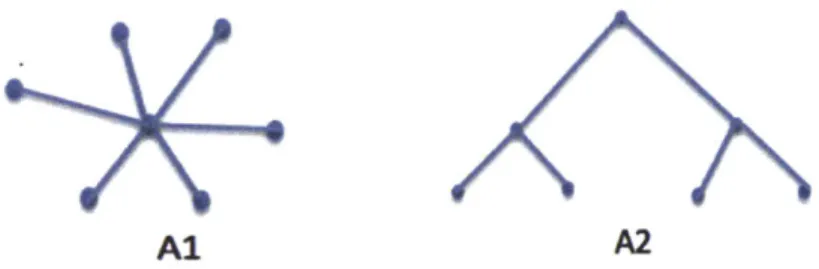
One of the key contributors to complexity is the internal architectural complexity of the system, and on the physical level that complexity is manifested through the interconnectedness of the system or subsystem. That internal complexity is

captured through the use of the Design Structure Matrix (DSM). Figure 4 represents three structural examples of increasing topological complexity. From left to right, these structures represent a centralized/bus architecture, a hierarchical architecture, and a distributed architecture. The degree of interconnectedness of the nodes is the chief differentiating factor leading to increased complexity in the C3 variable.

Increasing Topological Complexity

Figure 4: Topological Complexity

Measurement of the topological complexity in the ship's identified subsystem is captured via matrix energy. A property of matrix energy is that it is invariant to isomorphic transformations of the matrix, which makes it a suitable method for measuring the interconnectedness of the subsystem (Horn and Johnson 1994). The final topological complexity metric is defined by the energy of that adjacency matrix A E Mnxn.

(25)

The concept of matrix (or graph) energy was introduced by Ivan Gutman in 1978 as an aid for modeling the -electron energy of molecules. Gutman "formulated the a-electron energy of certain molecules as the sum of the absolute values of the eigenvalues of the adjacency matrix of a chemical graph associated with the molecular bonds." (diStefano and Davis 2009)

In each identified subsystem, A is the set of connected nodes in the DSM Ay. (Sinha and de Weck 2013)

Aij= 1, V[(i,j)I(i #

j)

and (ij) E A] 0, otherwise

The energy is given as follows based on Gutman's method and the standard eigenvalue equation (diStefano and Davis 2009):

n

E(Aij) = |A; A - AI = 0 i=1

Unidirectional interfaces only.

One of the chief limitations of the relatively simple summation of the absolute value of the eigenvalues is its lack of generalizability in undirected interfaces. In engineered systems, an undirected interface can be thought of as one in which data can flow multiple directions. For a physical system such as a welded joint, the system is directed, and with that system, the summation of eigenvalues would be sufficient, but in order to make this analysis as generalizable as possible, especially in regards to the analysis of advanced sensors and weaponry, the

summation ofsingular values via a singular value decomposition will be used in

(26)

n

E(Aij) = o;A - /1 = 0

Graph energy for Adjacency matrix Aij, containing a binary representation of generalizable, omnidirectional/undirected interfaces.

For the examples given below, A, would have an adjacency matrix represented by the following relatively sparse matrix given that only the central node has

connections to the others, while A2 has a slightly higher degree of connectivity

among the nodes:

0 1 1 1 1 1 1 0 1 1 0 0 0 0 1 0 0 0 0 0 0 1 0 0 1 1 0 0 1 1 0 O 1 1 A,1= 1 ...;A2 = 0 1 ~1o0

0o1~

1 0 0 0 000 0 0 1 0 0 0 0

From this equation one can calculate that ki = -2.45 and k2= 2.45 (all other

eigenvalues are 0) so E(A1) = 4.9. Following the same method, one can calculate

the notional E(A2) value is 6.83 (X1 = -2, k2= 2, ) = -1.41, k4 = 1.41,47 = 0) which is indicative of A2 being the more topographically complex structure by its

exhibition of a higher degree of inter-connectedness as shown in Figure 5, even though both structures A, and A2 have the same number of nodes and edges,

(27)

Al A2

Figure 5: Matrix Energy Nodal Structure Example

E (A) =

Z =

1-, where cy represents the ith singular value

C3 was equal to the matrix energy expressed from above times a normalization factor y based on the number of components.

C3 = y E(A), y = 1/n

In summary, structural complexity can be quantified via the integration of the discussed terms into the original equation for each subsystem targeted for analysis.

n n m

C(n, m, A) = xi + hjAi] yE(A)

i=1 = j=

As an illustrative example, Sinha and de Weck, 2013 showed that this analysis applied to two different jet engine architectures, "namely a dual spool direct-drive turbofan (e.g. new architecture) and a geared turbofan engine (e.g., new architecture)". After consulting with experts to collect data regarding interface complexity, it was determined structural complexity was underestimated by 43% since originally only the amount of connections

and pair-wise interfaces were considered. This resulted in a real 40% increase in complexity when only 28% was predicted thus contributing to an increase in development cost over the previous turbofan engine's predecessor.

(28)

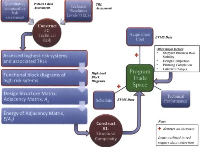
3. Information and Data Collection

All information and data collection efforts were seeking to answer the two main constructs that comprise the main premise of this study:

1. Complexity: The number of elements and interdependencies in the ship's architecture contributes to the ship's overall complexity.

2. Technical Risk: As a program management tool, technical risk is a key indicator of a program's self-assessed vulnerabilities. Those areas typically lie in areas of high complexity where the technology or employment of that technology is least understood. For example, a program with a requirement to employ a new radar will most likely assess that radar at a higher technical risk level than another shipboard system such as the hull.

This information is summarized in Figure 6.

PMaO/STbsk ArsskmeNt High l"d Block Diagraus EVMS Da Other MR WE facuwr& * Shipyard Bustness Base

Stability * Design Completion * Planning Completion - Contract Changes EVMS Da* Note:

+ denotes tin increase

Items outlined in red require data collection

(29)

3.1 Data Collection: Interviews

Interviews were conducted throughout the research at several different venues: organized shipyard tours, conferences, and appointments. A summary of the interviews, meetings, and travel conducted in support of this research is included in Appendix A. As the research progressed, the nature of the interviews evolved from seeking contextual and background information to seeking pertinent data and best practice information.

At the beginning of the research, the interviews and meetings helped refine and define what the course of the research would eventually be, and as the study progressed, the interviews became increasingly focused on data mining and gathering specific, targeted information on the subsystems under analysis. Of note, through the interviews with the Technical Director of PMS 400D2, a set of high-risk subsystems, their associated risk levels, and their functional block diagrams or drawings were obtained. This information fed directly into the logic and algorithms applied for analysis in Section 4.

3.2 Data Collection

Through the interviews with the Technical Director of PMS 400D, the three highest risk systems were identified as the AMDR, MRG, and the MCS. All of the particulars on why these subsystems were selected and their associated assessments are described in further detail in Appendix A. Following the methods described by Sinha and de Weck, 2013 in Section 2.3, the remaining data collection steps were to:

2 The Technical Director of PMS [Program Management (Ships)] 400D is the lead

technical government authority for HM&E (Hull, Mechanical, and Electrical) items in the DDG 51 program. Other systems such as Air Missile Defense Radar (AMDR) and

AEGIS are developed by other entities outside of PMS 400D. The DDG 51

government/contractor team then integrates those developed systems into the DDG 51 design.

(30)

* Assign values via expert assessment and field research for the X-vector leading to the determination of Ci.

e Gather the expert interface complexity assessment,

p

leading to the determination of C2.

- Collect the subsystem functional block diagram leading to the sequential determine of Aij, E(A), y, and C3 as described above.

3.2.1 Component Complexity Metric, Xi

The xi metric aggregates a complexity valuation for each subsystem based upon eight factors shown in vector X for each subsystem under analysis. It should be noted that the X-vector as it is presented was modified and adapted for the DDG 51-oriented case study

and is thus different from what was proposed in Sinha and de Weck's original work.

x1 x, - f (Performance Tolerance)

xW x = f(Performance Level)

x x = f (Component Size)

x x = f(Amount of Coupled Disciplines) C8(

XO -j 4 ; C1 = W(O = jx

xL x =

f

(Amount of Variables)

x x(0 = f(TRL)

x x(0 = f(Heritage Knowledge)

x~ x (0= f(Heritage Reuse)

The X vector3 was determined through a combination of expert assessments and other supporting research.

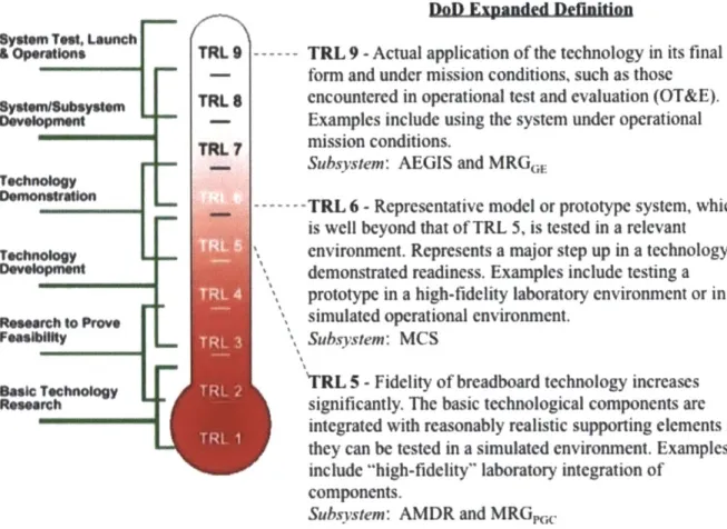
Given the ambiguity and DoD-centric nature of TRL, an expanded discussion is required of TRL and its effect on the X6 variable. As an adaptation to DoD

acquisition, the component reliability indicator, X6 was a function of the subsystem's

TRL. Each factor will be discussed in detail later, but TRLs were assessed based on

(31)

information from the interview with the PMS 400D Technical Director coupled with an integer-level corroboration per the DoD definitions for TRL. That information was mapped to the TRL level definitions provided in Figure 7 below.

DoD Ernanded Defitioue System Test, Launch

& Operstlons SystenVSubsystem Development Technology Demonsaton Technology Research to Prove Feasibility Basi Technooy Research TRL 9 --TRL G TRL 7

TRL 9 -Actual application of the technology in its final form and under mission conditions, such as those encountered in operational test and evaluation (OT&E). Examples include using the system under operational mission conditions.

Subsystem: AEGIS and MRGGE

- TRL 6 - Representative model or prototype system, which

is well beyond that of TRL 5, is tested in a relevant environment. Represents a major step up in a technology's demonstrated readiness. Examples include testing a prototype in a high-fidelity laboratory environment or in a simulated operational environment.

Subsystem: MCS

TRL 5 -Fidelity of breadboard technology increases significantly. The basic technological components are integrated with reasonably realistic supporting elements so they can be tested in a simulated environment. Examples include "high-fidelity" laboratory integration of

components.

Subsystem: AMDR and MRGpG.

Figure 7: TRL Level Definitions (NASA 2004) and Expanded Definitions (ASD R&E 2011)

Each subsystem's TRL was assessed based on the capability of the manufacturer producing that subsystem. For example, General Electric has historically produced the highly precise MRG for the DDG 51 class. When the Flight IIA line was restarted, GE announced that they would no longer be producing the MRG so a contract was let to provide the MRG as GFE for the continuation of the Flight IIA class. Philadelphia Gear Company (PGC) won the contract. When GE sent PGC the drawings for the MRG, PGC discovered that there was missing information in the technical drawings, and that some NRE and learning would exist until that knowledge gap between GE and PGC was

(32)

closed. In terms of TRL, an item that was TRL 9 for GE was a TRL 5 for PGC (Hellman 2013). According to DoD definitions (ASD R&E 2011):

* TRL 5 -Fidelity of breadboard technology increases significantly. The basic technological components are integrated with reasonably realistic supporting elements so they can be tested in a simulated environment. Examples include "high-fidelity" laboratory integration of components.

e TRL 6 -Representative model or prototype system, which is well beyond that of

TRL 5, is tested in a relevant environment. Represents a major step up in a technology's demonstrated readiness. Examples include testing a prototype in a high-fidelity laboratory environment or in a simulated operational environment. * TRL 9 -Actual application of the technology in its final form and under mission

conditions, such as those encountered in operational test and evaluation (OT&E). Examples include using the system under operational mission conditions.

TRLmax

6 _TRL.

Where 91(TRL) E [1,9] and TRL is each subsystem's assessed TRL based on the DoD standard definitions. Table 3 summarizes each subsystem's TRL and corresponding xi value.

Table 3: Subsystem Risk and x6 Values

AEGIS AN/AEGIS 9 1.0

Air and Missile Defense Radar (AMDR) 5 1.8

Main Reduction Gear (MRGGE) 9 1.0

MRGPGC 5 1.8

(33)

For reference, the X-vector definition is provided once more:

XM =

x = f (Performance Tolerance)

x = f (Performance Level)

x = f(Component Size)

x = f(Amount of Coupled Disciplines)

x = f (Amount of Variables) x = f(TRL)

x = f(Heritage Knowledge) x = f(Heritage Reuse)

The X-vector summary is shown in Table 4.

Table 4: X-Vector Summary (Normalized [0.,10] Value in Parenthesis) for a possible total Component Complexity score of 80

X1 9 9 6 10 10 X2 9 10 3 3 3 X3 7 7 3 2 2 X4 35 (10) 35 (10) 12(3.4) 1(0.1) 1(0.1) X5 35 (10) 35 (10) 31 (8.9) 27 (7.7) 27 (7.7) X6 2.0 2.8 2.5 2.0 2.8 X7 10 3 4 6 8 X8 10 4 3 5 9 .Xi 67 55.8 36.8 31.8 42.6

3.2.2 Interface Complexity Assessment,

p

(34)

complexity as described in Section 2.3. The director was asked to assess the interface complexity between 0 and 1 with 1 being the most complex interface one would see onboard a ship. An example of an interface that would garner a rating of 1 would be an interface with thousands of wires of varying voltages and frequencies. On the other end of the spectrum, an interface with a 0 rating would be quite simple, such as two plates bolted together. "If there were multiple types of connections between two components (say, load-transfer, material flow and control action flow), it would have a high

p value

since it would be more 'complex' to achieve/design this connection compared to a simpler load-transfer connection. For large, engineered complex systems, it appears that Pij in [0,1] is a good initial estimate." (Sinha and de Weck 2013)

Unfortunately due to governmental classification issues, it was impossible to assess each subsystem component's interface at a sufficient level of detail to assign

Pij

values for each interace within the subsystem. Detailed information on important subsystems such as AEGIS and AMDR are (justifiably) closely guarded secrets. Therefore, a simplying assumption had to be made in order to obtain reasonable values for Pij. It was determined that expert assessment, via the Technical Director for PMS 400D, would suffice to estimate the aggregated subsytem's interface complexity

f,

and that overarching

p

value would serve as the "rolled up" value for all the component interfaces within the

subsystem. While a realistic subsystem would most likely have interfaces of varying complexity, the assumption is that a qualified subject matter expert could estimate the overall average interface complexity. If the Navy chose to implement complexity-based cost estimation as shown in this study, this simplifying assumption could be immediately lifted to populate the

Pij

matrix without the constraints imposed by security concerns.

Table 5 below summarizes the findings for

Pij

for the three critical DDG 51 subsystems ranked via the PMS 400D interview and data collection process. These values were assumed to be the averaged value of all component interfaces contained within the subsystem, an assumption necessary because of the lack of visibility the researcher had into Navy subsystems because of the unclassified nature for which this study is intended.

(35)

Table 5: Subsystem Interface Complexity,

Pi

(Hellman 2013)

AEGIS AN/AEGIS 0.9

Air and Missile Defense Radar (AMDR) 1.0

Main Reduction Gear (MRG) 0.3

Machinery Control System (MCS) 0.8

3.2.3 Functional Block Diagrams and Schematics

Functional block diagrams were needed to create adjacency matrix models of the system from which the matrix energy could be derived per the methods laid out in Section 2.3.

Functional block diagrams were chosen instead ofphysical block diagrams due to a

subsystem's complexity being a matter of function more than parts. A subsystem could be comprised of a great number of parts while remaining relatively simple, while a different subsystem could be comprised of relatively few parts while being substantially more complex.

These diagrams led to a numerical result for C3 in the complexity equation.

AMDR and AEGIS

AMDR is slated to be the successor to the highly successful and prolific heritage AEGIS program. On October 1 0', 2013, Raytheon was awarded a $385+ million CPIF (Cost

Plus Incentive Fee) contract for the "engineering and modeling development phase design, development, integration, test, and delivery of Air and Missile Defense S-Band Radar (AMDR-S)." (Raytheon 2013). At the time of writing, AMDR-S and AMDR-X (X-band capable AMDR) will reportedly fall under separate contracts, and henceforth all references to AMDR will refer to AMDR-S.

(36)

Because of the classified and contractually sensitive nature of AMDR, unclassified, publically distributable data was scarce. To overcome this obstacle, the AEGIS (AMDR's immediate predecessor) was used as a case study to illustrate the complexity inherent in large multi-mission shipboard radars such as AEGIS and AMDR. In terms of power and cooling, AMDR will require substantially more of both; the current 200-ton cooling plant will be scaled up to a 300-ton plant that will provide cooling for the AMDR plus margin (Hellman 2013). Initially, the Flight III variant is slated to have a 14-foot AMDR that is the maximum size the DDG 51 deckhouse can accommodate, but eventually ship designs will be required to include the 20-foot AMDR to combat future ballistic missile threats.

A k-factor was required to quantitatively link AMDR to AEGIS in terms of complexity:

ComplexityAMDR = k CompleXityAEGIS.

To determine a reliable k factor, the key differences between AMDR and the traditional AEGIS radars must be examined. While AMDR has an expanded mission set over the less capable AEGIS predecessor, simply counting the missions would not necessarily yield a reliable k factor (based on a percent increase of missions) due to the fact that several missions are duplicated between the older AEGIS and the new AMDR.

Combining the qualitative interview assessment of increased AMDR complexity from PMS 400D with RAND Corporation's concept (RAND Corporation 2006) of power density (i.e., the ratio of power generation capacity to lightship weight), an electrical

power density-based k-factor was selected. Power density yields a more reliable metric

than just power because more power does not always yield more complexity. An old "muscle" car boasts more power than a modem luxury sedan, yet the modem luxury sedan has orders of magnitude more complexity than the old high-powered muscle car when one considers all the advanced technologies and software intrinsic to the new luxury vehicle. To compare power densities, one must consider the ship as a whole, and to facilitate the most reasonable "apples to apples" comparison, the DDG 51 Flight IIA, as the representative for the AEGIS case, and DDG 51 Flight III, as representative of the AMDR case, was selected. The differences between the ships in terms of length and non-radar centric power draws are minimal; chief differences lie within the non-radar subsystems

(37)

and the substantial power requirements of those radar subsystems. A k-factor was determined for AMDR using the definition and comparison equations presented below.

def Power Capacity

P"r _{= Lightship Weight}

_ PPwr,Ft.I _ 12.0 MW/9,600 LT

kAD = = = 1.52

PPwr,Flt.11A 7.5 MW/9,100 LT

Based on the observed power density increase, a k-factor of 1.52 was selected as the value estimated to yield the closest representation of the relative complexity increase in AMDR over AEGIS, for which there is substantially more unclassified and publishable data. Given that the k-factor functions as a coefficient adjunct to the C2C3 portion of the

complexity equation, any change in k yields a strictly linear change in net complexity so as more complexity-oriented data becomes publicly available, kAMDR can be dialed-in to a more accurate value. The relationships between k-factor and variations in Flight III's weight or power are shown in Figure 8. Variations are shown with respect to Flight III only; values for Flight IIA were held constant.

(38)

K-factor Scnsitivity Analysis in Flight II -Power Vaiation Weight Vaiation/ 100 2.5. 2.5 . 7 I- K . 1. ... I Variation

Figure 8: Sensitivity Analysis for AMDR K-Factor

At the time of writing only cost estimates exist for ships that will include AMDR, namely Flight III and beyond. The only actual costs that exist for AMDR are those in the

Research, Development, Test, and Acquisition (RDT&E) funds category so AMDR will be used for predictive cost measures while AEGIS will be used for methodology

validation using existing costs.

(39)

r

xw. -- -- - -- - TOU Akm

Ca I:

a

AIM Am

OF

(AC401_

.01y" o LPJ - N

[TV=

--- TOMAHAW s a wl

matrx shwn blow n Talew6

E(Aii=>LIt A-M=

(40)

It follows that:

Table 6: Adjacency Matrix, AAEGIS

E _Q S .5 -X z 5 Ri V5 8 .2 8S :3 2 3 3 3 4, 2

I

3 5 Excomn 0 10 10 0 10 0 10 0 10 10 10 10 0 10 0 10 0 10 0 0 0 10 1 1 0 10 1 1 1 1 0 0 10 0 10 10 Combat DF 0 *1 0 0 0 0 10 0 10 10 10 10 0 10 0 10 0 10 0 0 0 0 0 0 0 0 0 0 0 0 0 1 0 0 Surface Search Sys. 0 0 10 0 0 0 10 0 0 1 1 0 10 0 10 0 10 _0 0 0 0 0- 0 0 0 0 0 0 0 0 0 0 1 0 0 ES S 0 0 0 0 0 0 0 0 0 0 0 1 0 0 0 0 0 0 0 0 0 0 0 0 0 0 0 0 0 0 1 0 0 Navigation Sys. (Gyro) 0 0 0 0 0 0 0 0 0 0 0 0 0 0 0 0 0 0 0 0 0 0 0 0 0 0 0 0 0 0 0 1 0 0

IFF 0 0 6 0 0 0 0 0 0 0 0 0 0 0 0 0 0 0 0 0 0 0 0 0 0 0 0 0 0 0 0 1 0 0

SPY Radar System 0 0 0 0 0 10 0 0 0 0 0 0 0 0 10 0 0 0 0 0 0 1 0 1 0 0 6- 0 0 0 0 0 0 0 Hull Sonar System 0 0 0 0 0 0 0 0 0 0 1 0 0 0- 0 0 0 0 0 0 0 0 0 0- 0 0 0 -0 0 0 10 10 1 0 1

LAMPS Helo 0 0 0 0 10 0 0 0 0 0 1 0 0 0 0 0 0 0 0 0- 0 0 0 10 0 0 0 0 0 0 0 10 10 0 CEC 0 0 2 0 10 0 0 0 0 0 0 0 0 0 0 0 0 0 0 0 0 1 0 10 0 0 0 0 0 0. 0 1 0 0 uwSSQ-6LA(Sgnl) 0 0 0 0 0 a0 0 1 0 0 0 0 0 0 0 0 0 URTS/Q9LAN (inl 0 0 0 0 0 0 0 1 * 0 0 0 0 0 0 0 0 0 0 0 0 1 0 0 0 0 0 0 0 0 1 0 0 NRTX LE 0 0 0 0 0 0 10 0 0 0 0 0 0 0 0 0 0 0 0 0 0 2 1 0 0 0 0 0 0 0 0 1 0 0-UdrWS/Q- r A Direot~sp. 0 0 0 0 0 0 0 0 0 0 0 0 0 0 0 0 10 0 0 0 0 0 0 L 0 0 10 10 0 0 0 0 1 ArmIEd e 0 0 0 0 0 0 0 0 0 0 2 0 0 0 0 0 0 0 0 0 0 1 0 0 0 0 0 1 1 0 0 0 0 0 0 MUssdewtrFire ControlS. 0 0 0 0 0 0 0 0 0 0 0 0 0 1 0 0 0 0 0 0 0 0 1 0 0 0 0 0 0 0 0 0 1 0 0 AreVertclanh s 0 0 1 0 0 0 0 a 0 Rk a 0 0 0 1 a 0 0 0 0 0 1 0 0 0 0 0 0 10 10 0 0 0 0

Gissie Fie ontlSys. 0 01 0 01 0 0 0 0 0 0 0 0 0 0 a 0 0 0 0 0 0 1 0 0 0 0 0 0 0 0 0 0 0 0

AV.rtaHAK apuncys. 0 0 0 0 0 0 0 0 0 0 0 0 0 0 1 0 0 0 0 0 0 1 1 0 0 0 0 0 0 0 0 1 0 0 Eun e on afSys. 0 0 0 0 10 0 0 0 10 10 0 0 0 0 0 10 0 0 0 10 0 1 0 0- 0 0 0 0 1 0 0 0 1 0 1 Cdv. TOAHW WepnCt 0 0 0 0 0 0 0 0 0 0 0 0 0 10 0 0 0 10 0 10 10 0 0 0 0 1 0 0 10 0 0- 0 Ee nCD WfreSyAN . 0 0 0 0 0 0 0 0 0 0 0 0 0 0 0 0 0 0 0 0 0 110 0 0 0 0 0 0 0 10 0 0 0 FTSW AN 0 0 -0 0 0 0 0 1 0 0 0 0 I 1 z 0 0 1 10 0 0 0 0 0 0 0 0 1 0 1 0 1 BFT0 0 _{0 0 0 0 0 0 0 0 0 0 0} _DI ATCS LA 0 0 -L 0 0 0 0 0 0 0 0 0 0 0 0 0 0 0 0 0 0 a 0 0 0 0 0 0 0 0 0 0 1 CDNetwork0 0 0 0 0 0 1 0 0 0 0 0 0 0 0 0 0 0 0 0 0 0 0 0 0 0 0 0 0 1 1 ADS 0 0 0 0 0 0 0 0 0 0 0 0 0 0 0 0 0 0 0 0 0 0 1 0 0 0 0 0 0 0 " 1 0 10 AGS LAN n1cnnc~s 0 0 0 0 0 0 0 0 0 0 0 0 0 0 0 0 0 0 0 0 0 0 0 0 0 0 0 0d 0 0d 0 0 2 C2P2 0 0 0 00 00 0 10 00 00 0 00 00 1 00 r1

CDM AEG0 S n=0:34 = [485 4.66 20 0 .. ] E0AEI 0000 AEGI0000S

-inr ada0c 0h mari AAG0 0 0/3 ) = 0 02 an C3 = 0 E(AAEGIS0 0 -9

aEtLAIcnneyc t Syse (MC0S) n1n

The MCS "provides a centralized means of monitoring and controlling the main

propulsion plant, electric plant, and auxiliary systems" (Cairns 2011) onboard the DDG 51 class. Like the AEGIS and AMDR subsystems, MCS's complexity is derived from the amount of interfaces, the complexity of those interfaces, and the complexity of the

Z

0