A continuum model for phase transitions in thermoelastic solids and its application to shape memory alloys

A Continuum Model for Phase Transitions

in Thermoelastic Solids

and Its Application to Shape Memory Alloys

by

Sang-Joo Kim B.S., Naval Architecture Seoul National University (1984)

M.S., Naval Architecture Seoul National University (1986)

Submitted to the Department of Mechanical Engineering in partial fulfillment of the requirements for the degree of

Doctor of Philosophy in Mechanical Engineering

at the

MASSACHUSETTS INSTITUTE OF TECHNOLOGY

February, 1995

(Massachusetts Institute of Technology 1995. All rights reserved.

Author

Ah UV Department of Mechanical Engineering

August 4, 1994

Certified by

-.

-Professor Rohan Abeyaratne Thesis Supervisor

Accepted by .-

Chairman Departmental Committee on Graduate Studies

A Continuum Model for Phase Transitions

in Thermoelastic Solids

and Its Application to Shape Memory Alloys

by

Sang-Joo Kim

Submitted to the Department of Mechanical Engineering on August 4, 1994, in partial fulfillment of the requirements for

the degree of Doctor of Philosophy in Mechanical Engineering

Abstract

Thermoelasticity theory has been used to study certain general issues pertaining to solids that undergo reversible stress- and temperature-induced phase transforma-tions. A complete constitutive theory that describes the behavior of such materials consists of a Helmholtz free-energy function which describes the response of each in-dividual phase, a nucleation criterion which determines when a phase transition is initiated and how many nucleations occur, and a kinetic relation which characterizes

the speed at which a phase boundary moves.

This thesis is focused on the construction of an explicit one-dimensional con-tinuum model of such materials and its application to Ni-Ti shape memory alloys, and it can be divided into four parts. First, a complete one-dimensional constitutive model is constructed. The Helmholtz free-energy function here has three energy wells associated with austenite and two variants of martensite. The nucleation criterion describes the nucleation of multiple phase boundaries based on some experimental observations; it signals the conditions under which the transition from one phase to another commences based on a critical value of driving force. Two examples of kinetic relations are introduced; one is based on thermal activation theory and the other is based on experimental observation. Secondly, the thermomechanical predictions of the model are calculated and qualitatively compared with experiments. A numerical algorithm is developed to solve a movin.: boundary problem associated with stress-induced transformations by combining a standard finite difference method with a Lagrangian interpolation equation. Thirdly, the Helmholtz free-energy function is modified to take into account the effect of cyclic loading and unloading on the trans-formation characteristics of the material. Two internal variables are added to the energy function to describe the changes in the free energy of the martensite phases during phase transformations. It turns out that this model simulates successfully various cyclic effects such as the two-way shape memory effect. Finally, the model is used to simulate recent experiments on NiTi shape memory wires. The predictions of the model are in quantitative agreement with experimental observations.

Thesis Supervisor: Dr. Rohan Abeyaratne Title: Associate Professor of Mechanical Engineering

Acknowledgments

I would like to express my sincere gratitude to my thesis advisor, Professor Ro-han Abeyaratne, for his support, patience, and insightful guidance through the course of this research. I also wish to thank my committee members, Professors James K. Knowles and Stuart B. Brown, for their comments and suggestions which helped im-prove this thesis.

I am grateful to Professor S. Kyriakides and Mr. J. Shaw of the University of Texas at Austin for providing me with their data for Nitinol that I use in Chapter 8 and also for some helpful discussion. The useful discussion with Professor S. M. Allen in the Department of Materials Science and Engineering is also appreciated.

I give my thanks to my colleagues, Dr. Yier Lin and Alfred Pettinger, for the many conversations we have had. Also, I appreciate the friendship and support of all my friends at MIT for the last five years, especially Drs. Hyun Yup Lee, Hee Chun Song, Woojae Seong, Yun-Jae Kim, Hyungyil Lee, Jahng Hyon Park, Hyunjune Yim, :Hyun Seok Yang, Jangbum Chai, and many others.

I am most indebted to my parents, who supported me throughout my life in all ways they could; special thanks go to my father-in-law and late mother-in-law for their encouragement and concern. At last, but not least, I want to thank my wife for her patient encouragement and love. Without her devotion, this work could never have been done.

The initial period of my graduate studies was supported by the Army Research Office, while the latter period was supported by the National Science Foundation. I am grateful for this support.

Table of contents

Abstract 2

Acknowledgments 3

Table of contents 4

1 Introduction 7

1.1 Thermoelastic martensitic phase transformation ... 7

1.2 Review of continuum modeling . . . 9

1.3 Outline of thesis ... 12

One-Dimensional Continuum Model

3.2 Construction of three-phase ... 23

3.3 Driving force and latent heat ... 27

Appendix ... 30

4 Nucleation Criterion and Kinetics 37 4.1 Nucleation criterion ... 37

Thermomechanical Response of the Model

5 Isothermal Thermomechanical Response 50

5.1 An example of isothermal thermomechanical response ... 50

5.2 Material parameters ... 51

5.3 Results and discussion ... 5... 52

6 Thermomechanical response with heat transfer 62 6.1 Introduction . . . ... 62

6.2 Macroscopic thermomechanical response ... 63

6.3 Nondimensionalization ... 66

6.4 Finite Difference Method ... 67

6.5 Accuracy of program ... 69

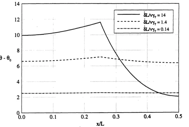
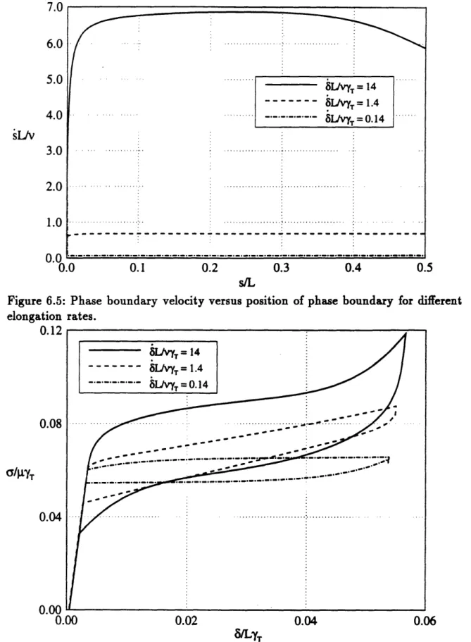
6.6 Results and discussion ... 71

Cyclic Effects

7.2 Nucleation and evolution ... 84

Experimental Verification of the Model

8 Experimental Verification of the Model for NiTi Wires

103

8.1 Material parameters ... 103

8.2 Results and discussion ... 107

9 Concluding Remarks 121

Chapter 1

Introduction

1.1 Thermoelastic martensitic phase

transforma-tion

Of the several solid state phase transformations occurring in alloy systems, marten-sitic transformations have had a very special interest to researchers. In the early years this interest arose out of the extraordinary hardness that iron-carbon marten-site possessed. Soon it was realized that a number of alloy systems, both ferrous and nonferrous, exhibited martensitic transformations and these have been the subject of innumerable investigations. Special emphasis was laid on the fact that the resultant

martensite phase had a common interface with the parent phase that was both undis-torted and unrotated. This also led to the emergence of the phenomenological the-ories to account for the observed crystallography of the parent-product relationship.

Recently, however, the observed overall characteristics of the martensitic transforma-tions have been used by Cohen et al. (1979) to define a martensitic transformation as one where (a) there is a lattice deformation with an accompanying shape change, (b) diffusion is not required and (c) the kinetics and morphology during the trans-formation are dominated by the transtrans-formation strain energy. Therefore, martensitic transformations can be induced by the application of stress as well as by changes in temperature and they are crystallographically reversible. Usually, the shape deforma-tion of a martensitic transformadeforma-tion is so large relative to the stiffness and strength of the surrounding parent phase that plastic accommodation takes place during the growth process. In this sense, the interfacial motions are not reversible. Alternatively, in those instances where the shape deformation can be accommodated elastically, the interfacial motions take on reversible features. In this thesis we will consider the latter

case only, so that no plastic deformation is induced during the transformation. Then the characteristics of martensitic transformation that are mentioned can sometimes lead to some interesting effects: thermoelasticity, pseudoelasticity, shape memory ef-fect and two-way shape memory efef-fect.

A thermoelastic martensitic transformation is realized if martensite forms and

grows continuously as temperature is lowered, and shrinks and vanishes continuously as temperature is raised. In their experiments with an In-TI single crystal alloy, Burkart and Read (1953) observed a single interface separating the parent phase and the product phase. On slow cooling, the specimen transformed from the face-centered

cubic structure to the face-centered tetragonal structure at the martensite start

tem-perature M. by the motion of a single plane interface which traversed the specimen from one end to the other. Upon heating, the interface moved back in the reverse di-rection. Other alloys which exhibit thermoelastic transformation are AgCd, CuAlNi,

NiTi, CuZn, CuSn, InTI, and so on.

Alloy systems which undergo a thermoelastic transformation on cooling can be made to transform in a similarly reversible manner, even at temperatures above M,, by applying an increasing stress. This type of stress-induced transformation is an example of pseudoelasticity in view of the relatively large deformation that can be manifested (~ 10 %) by the induced transformation, and yet this strain is "elas-tically" recoverable on unloading due to the reversal of the transformation. Many interesting features of the pseudoelastic behavior has been found. The shape of the stress-strain curve depends heavily on temperature and the stress necessary for trans-formation is found to increase with temperature (see Krishnan (1985), Kyriakides et al. (1993)).

The shape memory effect arises if a macroscopic deformation is accompanied, as before, by a martensitic transformation at a temperature lower than the transfor-mation temperature; in a second step the reverse transfortransfor-mation and a concomitant reversal of the macroscopic deformation are induced by heating up to a temperature higher than the austenite finish temperature Af. The system recovers its original shape after heating.

Up to this point we have implied that pseudoelasticity and the shape memory effect were associated with a martensitic transformation. The same phenomena can occur even when the specimen is fully martensitic at the outset. In this case the macroscopic deformation is induced by reorientation of martensites. Thus, pseudoe-lasticity and the shape memory effect may be associated with a martensitic transfor-mation, a reorientation of a martensitic structure or a combination of both.

The shape memory effect just considered is one-way, i.e. no appreciable change in specimen shape occurs during the martensitic transformation on cooling; instead, a change in shape takes place during the reverse transformation on heating above

Af which cancels the prior change of shape introduced by deforming the specimen.

In the two-way shape memory effect, an overall change of specimen shape operates during the cooling and heating transformations. The condition can be brought about in two ways: either after pseudoelastically cycling by loading and unloading several times above the transformation temperature or by going through the one-way shape memory effect a number of times. It appears that both of the above "training" meth-ods, i.e. by stress induced martensite (SIM) cycling or by shape memory effect (SME) cycling, involve the preferential formation of lattice defects or micro-stresses which favor selected variants during the thermoelastic transformation on cooling.

1.2 Review of continuum modeling

Various continuum-level issues related to martensitic phase transformation in crys-talline solids have been successfully studied using the theory of finite thermoelasticity. For a thermoelastic material, the Helmholtz free-energy function 0i depends only on the deformation gradient tensor F and the temperature : = p(F, 0). If the stress-free material can exist in two phases, then the energy function

4,

T, the two phases have the same energy. For > T the austenite minimum is smaller, while for < T, the martensite minimum is smaller. In the

presence of stress S, one must consider the potential energy function G = G(F; S, 9) involving the energy wells, where S is the first Piola-Kirchhoff stress tensor. Now the material can have different stable phases co

responding to different combinations of applied stress and temperature.

Much recent activity in continuum mechanical studies on thermoelastic phase transformation has been focused on two basic issues: the first concerns the

equilib-rium configurations of a body corresponding to the stable state; the second is related

to the non-equilibrium evolution of a body from metastable states to stable states.

Ericksen (1975) studied energy minimizing deformations for a two-phase mate-rial within the one-dimensional mechanical setting of a tensile bar. He showed, in particular, that for certain values of prescribed displacement, the stable equilibrium configurations of the bar involve co-ezistent phases. The analogous issue in higher dimensions is more complicated: typically, deformation gradient tensors Fa and Fm corresponding to the austenite and martensite energy minima are not kinematically compatible with each other, i.e. Fa - F, is not a rank-one tensor. Therefore an en-ergy minimizing deformation cannot correspond to homogeneously deformed states of austenite and martensite separated by a phase boundary. In fact, an energy minimizer usually does not even exist, and one must contend with minimizing sequences. The deformation pattern associated with such a sequence characterizes the underlying mi-crostructure of the material; in Cu-Al-Ni for example, an austenite-martensite phase boundary separates a homogeneous state of austenite from a fine mixture of twinned martensite. These ideas were put forward by Khachaturian and Shatalov (1969) and Roitburd (1978) using a geometrically linear theory, and by Ball and James (1987) for the finite deformation theory; see Bhattacharya (1991b) for a comparison of these two theories. Ball and James (1987) studied an austenite/twinned martensite interface in detail, and showed that the consequences of their theory are in agreement with the crystallographic theory of martensite which is a classical theory that is not based on the idea of energy minimization. Needle-like microstructures and self-accommodating microstructures have been explored by Bhattacharya (1991a) using similar ideas. The fineness of the microstructure is controlled by surface energy, though the effects of surface energy may be more subtle than this; e.g. see Gurtin and Struthers (1990) and Kohn and Miiller (1991).

The usual continuum theory of thermoelasticity, though adequate for charac-terizing two-phase energy minimizers, does not characterize quasi-static or dynamic

processes of a body involving transitions from one phase to another. This is illustrated by the tremendous lack of uniqueness of solution to particular initial-boundary-value

problems in the works of Abeyaratne and Knowles (1988, 1991). In order to solve this

uniqueness problem they adopted the view that the lack of uniqueness in the con-ventional formulations arose from a constitutive deficiency associated with particles on the phase interface and they supplemented the theory with further constitutive information, which were a kinetic relation and an nucleation criterion. The kinetic relation controls the progress of the phase transition once it has commenced and the nucleation criterion signals the initiation of a transition. Thus a complete consti-tutive theory which is capable of modeling processes involving thermoelastic phase transitions consists of a Helmholtz free-energy function, a kinetic relation, and a nu-cleation criterion. Abeyaratne and Knowles (1988, 1991) showed that the particular initial-boundary-value problems have unique solutions when studied in this broad-ened setting.

A number of studies have been concerned with developing explicit constitutive models. For example, Ericksen (1986) and Silling (1989) have constructed three-dimensional Helmholtz free-energy functions for modeling certain crystals; Falk (1980) has studied a one-dimensional polynomial free-energy function, see also Jiang (1989). Models of kinetic relations have been constructed, for example, by Muller and Wilman-sky (1981) using certain statistical considerations, and by Otsuka et al. (1976), by assuming phase-boundary motion to be similar to dislocation motion. Abeyaratne and Knowles (1993) constructed a complete, explicit one-dimensional model for describ-ing thermoelastic phase transformations, which consists of a Helmholtz free-energy function having two energy wells, a kinetic relation based on the notion of thermal activation, and the nucleation criterion signalling the initiation of transition based on the critical value of driving force.

Recent experiments by Kyriakides and Shaw (1993) have suggested that local heat transfer effects can be very important. For example, when they carried out iden-tical tests at ideniden-tical environment temperature, the response was found to be quite different depending on whether the environment was water or air. This is probably due to the different heat transfer characteristics of these two media. Some investigations on the effect of the heat of transformation on a stress-induced phase transition have

been carried out. For example, Petukhov and Estrin (1980) have studied the steady state motion of a phase boundary in an infinite bar. Grujicic, Olson and Owen (1985) measured the temperature change during the phase transformation of a Cu-AI-Ni sin-gle crystal and carried out a theoretical analysis of a related heat transfer problem. Rodriguez and Brown (1975) measured temperatures during the forward and reverse transitions of a Cu-AI-Ni single crystal and discussed the effect of elongation-rate on the stress-elongation curves. Recently, Leo, Shield and Bruno (1993) carried out a detailed and informative study in which they conducted experiments on a Ni-Ti shape-memory wire and used a theoretical model to explain their observations.

It has been noted by many researchers that the characteristics of thermoelastic martensitic phase transformation are changed when the transformation is repeated many times by thermal and stress cycling. This is because, during thermomechanical cycling, phase boundaries travel forward and backward in the specimen and some mi-crostructural defects such as dislocations are generated and distributed in the alloy; for example, see Melton and Mercier (1979), Perkins and Sponholz (1984), Miyazaki et al. (1986a, b), and so on. A continuum model to describe the cyclic behavior of shape memory alloys was proposed by Tanaka et al. (1992, 1994). They took the point of view that the dislocations generated are a primary cause of the accumulation of a microscopic residual stress and strain in the alloy. They introduced three internal variables, i.e. the microscopic residual stress and strain and the volume fraction of

the residual martensite.

1.3 Outline of thesis

This thesis is divided into four parts: the construction of a continuum model, the thermomechanical response of the model, the incorporation of cyclic effects into the model, and the application of the model to experiments.

The discussion on the construction of a continuum model is given in Chapters 2, 3 and 4. In Chapter 2 we outline the general theoretical framework within which the model will be constructed. In Chapter 3 an explicit Helmholtz free energy function having three energy wells corresponding to austenite and two variants of martensite

is constructed. Chapter 4 is devoted to the description of a nucleation criterion and a kinetic relation. The nucleation criterion consists of two parts: one is associated with the instant of initiation of a transition, the other is associated with the nucleation of multiple interfaces throughout the transition. Two kinetic relations are used in this thesis: one is derived from thermal activation theory, the other is a linear one with some range of driving force over which the speed of phase boundary is zero.

Next we use the explicit forms of the constitutive equations to obtain the thermo-mechanical response of the model. In Chapter 5 we calculate the various predictions of the model under the assumption that the thermomechanical processes considered are so slow that the temperature at any particle on the bar is equal to that of the environment at any time of the process. In Chapter 6 we give up the assumption of isothermality and carry out a numerical analysis to solve a moving boundary prob-lem associated with stress-induced phase transformations. A numerical algorithm is developed to solve this non-trivial problem by combining a standard finite difference scheme with a Lagrangian interpolation equation. Attention is focused on how the response is affected by the heat generated during the transformation.

Chapter 7 deals with the incorporation of cyclic effects into our model. Some microdefects are generated as phase boundaries migrate through the material and they form a stress field which favors a particular phase. We take the point of view that the free energy of the phases varies due to the introduction of the microdefects. In order to take into account the associated changes in stability of the phases, two internal variables are added to the Helmholtz free energy function. It turns out that this modified model successfully simulates various cyclic effects.

Finally, in Chapter 8, the model is used to simulate the recent experiments on a

Ni-Ti shape memory wire by Kyriakides and Shaw (1993). They have done many

ex-periments under various testing conditions. The effects of temperature, environmental conditions, elongation rates, cyclic loading on the global mechanical response of the wire have been investigated. The temperatures and strains at different points along the wire were measured during the phase transformation too. Their experiments give us a good chance to verify our model.

One-Dimensional

Continuum Model

Abstract

We construct an explicit constitutive model that is capable of describing the ther-momechanical response of a shape-memory alloy. The model consists of a Helmholtz free-energy function, a nucleation criterion and a kinetic relation. In Chapter 2 we re-view some basic concepts from the continuum theory of thermomechanical processes within a purely one-dimensional setting; in Chapter 3 we construct a free-energy func-tion having three energy wells associated with austenite and two variants of martensite respectively; in Chapter 4 we discuss a nucleation criterion and a kinetic relation, the former tells us when a transition is initiated and how many interfaces are nucleated and the latter tells us how fast a phase boundary propagates.

Chapter 2

Theoretical Framework

Consider a uniform specimen with length L, cross-sectional area A and mass density p in a reference configuration. The specimen is contained in an environment whose temperature is

e

interval [0, L] of the -axis in this configuration. When the bar is stretched to an equilibrium state, the displacement u(z, t) is assumed to be continuous and piecewise smooth. The bar is modeled as a thermoelastic solid, with a given Helmholtz free en-ergy function ?k(, 0) per unit mass; = O8(, t) is the absolute temperature, assumed to be continuous and piecewise smooth, and y = '(,t) is the longitudinal strain, both at the particle whose Lagrangian coordinate is and at time t. We require the strain to satisfy > -1, so that the deformation is one-to-one.

For a thermoelastic material the stress and entropy per unit mass 77 at a particle are constitutively related to y and by

= (7, ) = pi,(, ), 77 = (IY, ) = -be( 7, ). (2.1)

The potential energy per unit reference volume G(7; 8, a) of the material is defined

by

G(

;

e,

a) = p(

7

,

) -

ay,

(2.2)

and its value at an extremum of G(9; 8, a) coincides with the Gibbs free energy per unit reference volume:

In order to model a material that can undergo a thermoelastic phase transition G(e; 0, a) should have multiple local minima ("energy-wells") when the temperature and stress take on suitable values; the corresponding Helmholtz free-energy potential

(., 8) will be non-convex, and the stress-strain curve characterized by a = p.,(y, 8)

will be non-monotonic. In this theory, each local minimum of the potential energy function G, and therefore each branch with positive slope of the stress-strain curve, is identified with a different (metastable) phase of the material.

Suppose that G(e; 8, a) has at least two local minima corresponding to a given temperature 0 and stress oa, and let a =7=y (8, oa) and y =7=7 (8, oa) denote the

val-ues of strain at these two energy-wells. Then the strain at a particle that is subjected to this and a could be either 7 or y depending on which energy-well (i.e. phase) the particle is in. Let x = s(t) denote the current location in the reference configuration of a particular particle of a bar; suppose that the particle immediately to the left of

x = s(t) has a strain 7 while the strain on its right is y; then x = s(t) denotes the

location of a phase boundary, i.e. an interface that separates two distinct phases of

the material.

At each instant t during a slow thermomechanical process, the strain 7(z, t) and temperature gradient 8,(x, t) vary smoothly within the bar except at phase bound-aries; across a phase boundary, they suffer jump discontinuities. The displacement and temperature fields are assumed to remain continuous throughout the bar. Away from a phase boundary, mechanical equilibrium and the first and second laws of

ther-modynamics require that

az = O, -q + pr = pO77t, qO < O, (2.4) respectively, where q(x, t) is the heat flux in the +x-direction and r(z,t) is the heat supply rate (to the bar) per unit mass. At a phase boundary x = s(t), one has the associated jump conditions

+-

= 0, q - q= f + p(t7 -

[0,

(2.5)

where f is the driving force on the phase boundary defined by

In (2.5) and (2.6) we have written h=h (t) = h(s(t)±,t) for the limiting values of a field h(x, t) as the phase boundary x = s(t) is approached from either side. In the present setting, the driving force also equals the jump in Gibbs free-energy across the phase boundary:

f = G(4;

6,

6,

If the driving force f happens to vanish, one speaks of the states (, 0) and (, 0) as being in "phase equilibrium" and of the quasi-static process as taking place "re-versibly". If G(}; 0, a) > G(7; , a), then f is positive and so according to (2.5)3 one has > 0; thus if the phase boundary propagates, it moves into the positive

side and thereby transforms particles from (, 0) to (7,0). In this sense, the mate-rial prefers the smaller minimum of G. This is also true in the reverse case when

G(';; 0, o) < G(7; 0, ). One therefore speaks of the phase associated with the lowest

energy-well as being the stable phase.

By using the first law of thermodynamics in (2.4) and (2.5) one can show that the heat generated when a unit mass of material changes phase from (, 0) to (7, 0) is f/p + A where A = (77 - 77) is the latent heat; if the phase change occurs under

conditions of phase equilibrium, then f = 0, and the heat generated is A.

Let x = s(t) denote the Lagrangian location of a phase boundary at time t. As particles cross this interface, they transform from one phase to another at a rate that is determined by the underlying "kinetics". The kinetics of the transformation control the rate of mass flux pi across the phase boundary. If one assumes that this flux depends only on the states (7, 0) and (', 0) on either side of the interface, then the propagation of the phase boundary is governed by a relation of the form

A = v(7, 0,9), (2.8)

where the kinetic response function v is determined by the material. Alternatively,

since the constitutive relations a = p,(r(7,6) and = py('7,0) can be inverted

(separately) for each phase, one can express and 7 in terms of a and , and thus re-write the kinetic law (2.8) in the form

where the function v depends on the two particular phases involved in the transfor-mation and is different for each pair of phases. Finally, by substituting the inverted stress-strain-temperature relations into (2.6) one can express the driving force acting on an interface between a given pair of phases as f = f(0, a); this in turn can be inverted at each fixed , and so the kinetic law can be expressed in the form

= V(f, ).

(2.10)

The basic principles of the continuum theory do not provide any further information regarding the kinetic response functions V; in particular, explicit examples of V must be supplied by suitable micromechanical constitutive modeling.

Next, consider a quasi-static process during which the bar involves only a sin-gle phase of the material for some initial interval of time, and two distinct phases at subsequent times. The kinetic law (2.10) describes the evolution of ezisting phase boundaries and therefore is only operational once the bar is in a two-phase state. The

initial transition of the bar from a single-phase configuration to a two-phase

configu-ration and the number of phase boundaries nucleated after the initiation instant are controlled by a nucleation criterion. The particular nucleation criterion that we shall use in the thesis will be described in Chapter 4.

In addition we also have a heat conduction law

q = -k( ₇, 8)8,, (2.11)

which governs the flux of heat at points away from a phase boundary and the heat conductivity k is characteristic of the material.

The heat supply term r, in the present one dimensional study, models the transfer of heat through the lateral surface of the bar, for which there are two mechanisms: convection and radiation. We shall take the former to be controlled by Newton's law of cooling and the latter by Stefan-Boltzmann law. Then

r(x,t)

=

-¢C[(x,

t) - 8o(t)] - C,[84(x,t)

- eo(t)],

(2.12)

where

C,

4,

to give

r(x,t) = -(t)[O(x,t)- Oo(t)], (2.13)

where C(t) = -[C¢ + 4¢C03(t)].

We also need to describe the thermal and mechanical boundary conditions at the ends of the bar. With regard to the former, we suppose that the rate at which heat is transferred from either end of the bar into the surrounding medium is governed by Newton's law of cooling, so that

k0o(O,t) = A[e(o,t)-0o(t)],

kO(L,t) = -a[O(L,t)

o(t)],

(2.14)

where > > 0 is a constant and Oo(t) is the temperature of the environment; the special cases = 0 and = oo correspond to the respective cases where the ends of the bar are perfectly insulated and have prescribed temperature ₀o(t).

Suppose that one end of the bar is always held fixed, that is,

u(0,t) =

0,

then there are two possibilities for the boundary condition of the other end. In a hard device the position u(L, t) is determined by an applied elongation 6(t), so that

u(L, t) = 6(t). (2.16)

In a soft device the stress a(L, t) is determined by an applied stress ao(t), so that

Chapter 3

Helmholtz Free-Energy Function

We start this chapter with a brief discussion of some qualitative features of the specific one-dimensional model that is to be constructed in this chapter. Suppose for purposes

of discussion that the material at hand exists in a cubic phase (austenite or A) and an orthorhombic phase (martensite or M); an example of this is the class of Cu-AI-Ni shape memory alloys. The associated (three-dimensional) potential energy function G must have seven energy-wells corresponding to the austenite phase and the six "variants" of martensite. During a uniaxial test of a single crystal specimen, and for suitable values of temperature , the material is found to remain in the cubic phase (phase A) for sufficiently small values of stress, in the orthorhombic phase yielding the largest elongation for sufficient large tensile stresses, and in the orthorhombic phase giving the largest contraction for sufficiently large compressive stresses. In a one-dimensional theory we model this by allowing G to have three energy-wells for suitable and , the ones at the largest and smallest values of strain correspond to the two variants M+ and M- of martensite just described, while the one at the inter-mediate value of strain is identified with austenite. Since the variants of martensite are crystallographically identical to each other when = 0, the energy-wells corre-sponding to them are required to have the same height at all temperatures whenever the stress vanishes. Moreover, all three energy-wells should have the same height if the stress vanishes and the temperature coincides with the transformation temperature

aT. At higher temperatures, the austenite is preferred over the martensite, and so the model should be such that the austenite energy-well is lower than the martensite wells when > T; the reverse for < T. The crystallographic similarity between the variants also suggests that the specific entropy associated with them should be identical, and therefore that the latent heat associated with the transformation from

one martensite variant to the other should be zero; this too is a feature of our model.

A note on terminology: for simplicity of presentation we shall sometimes speak of "three phases" rather than the "one phase and two variants"; similarly we shall often use the term "phase boundary" generically to refer to both an interface between two phases and to an interface between two variants (which ought to be called a twin boundary); also we shall sometimes use the term "forward" transformation for the

A -, M+ and A -, M- transformations, and the term "reverse" for the M+ - A

and M- - A transformations.

3.1 A single-phase thermoelastic material

Consider a uniform bar which, in a reference configuration, has length L, cross-sectional area A and mass density p. The ends of the bar are subjected to axial forces oa(t)A and the bar is contained in an environment whose temperature is (t). Suppose that the bar is in a uniform state. The Helmholtz free-energy of the bar per unit mass and the Gibbs free-energy of the bar per unit reference volume are defined by

+(t) = (t)

-(t)(t),

(3.1)

g(t) = pb(t) -

(t)

(t),

(3.2)

where 7(t), e(t) and 7(t) are the strain in the bar, the internal energy of the bar per

unit mass and the internal entropy of the bar per unit mass respectively. The stress at every particle in the bar is cr(t) and all equilibrium requirements are automatically satisfied. Applying the first and second laws of thermodynamics and rearranging terms

gives

Q = (p - j)LA, (3.3)

r

=

P -

p

-

LA,

(3.4)

where Q and

r

Suppose next that this bar is made of a thermoelastic material:

Then by using (3.1), (3.3), (3.4) and (3.5) we get

Q = peOLA,

r =0.

Using (3.5)3 in (3.6)1 gives Q = p0(-,/Oej - ooe)LA.9

Now consider a special process during which y(t) = constant. Then Q = -po'ooeeLA. The specific heat at constant strain, c = Q/(pLAe), can therefore be expressed as

c-, ) = -poo(

, 0).

(3.8) Consider a special process during which a(t) = constant. Then the coefficient of

thermal expansion, a = i/@, can be expressed as

a(-Y, ) = - , (, ) (3.9)

Now we consider a (single-phase) thermoelastic material for which the modulus

A, the coefficient of thermal expansion a and the specific heat at constant strain c

are all absolute constants:

J

A

for all

7,

0,

pob(7y, 0) = (/2)(7 - g.) - a70 + pc(O - 0log(0/0.)) + p*. for all 7, 0, (3.11)

where g*, 0* and ,>. are constants. This Helmholtz free-energy function holds at every point on the (, 0)-plane and has only one energy minimum on that plane.

3.2 Construction of three-phase

4

In this section by using (3.11) we construct an explicit three-well Helmholtz free-energy function ib(₇, 0) that characterizes the response of a multi-phase material; the

three energy-wells are viewed as corresponding to an austenitic phase and to two variants of martensite.

Consider a material which exists in a high-temperature phase austenite (A) and as two variants (M+ and M-) of a low-temperature phase martensite. Suppose for

simplicity that the austenite and both martensitic variants have the same constant

elastic modulus p > 0, the same constant coefficient of thermal expansion a > 0 and the same constant specific heat c > 0. (The model that follows can be readily gen-eralized to describe the case wherein the different phases have different but constant material properties.) Suppose the free-energy function (3.11) derived in the previous section holds only on some domain of the (, 0)-plane, then the Helmholtz free-energy function k(y, 0) associated with this material has the form

(j/2)(7

- 91g)2

-

+

pc(9

-

Elog(/

)) + po,

on P

,

p'b

(/2)(7

parT

,

(j/2)(y

where p is the mass density of the material in the reference configuration, and Oi,

gi, bi, i = 1, 2, 3, are nine additional constants whose physical significance will be

made clear in what follows. The regions P1, P2 and P3 of the (Y7,0)-plane on which

the three expressions in (3.12) hold are the regions on which the respective phases A,

M+ and M- exist; they are assumed to have the form shown in Figure 3.1, where in

particular the boundaries of P1, P2 and P3 have been taken to be straight lines. The

temperature levels ,,9 _{and M denote two critical values of temperature: for 0 > M}

the material only exists in its austenite form, whereas for < O, the material only exists in its martensite forms. Throughout this paper we will restrict attention to

temperatures less than aM.

We now impose a number of restrictions on ib in order that it properly model the stress-free response of the material we have in mind. Since the potential energy function G and the Helmholtz energy function 'b coincide when the stress vanishes, any characteristic to be assigned to G at = 0 could be equivalently imposed on b.

Let ,m and OM be the two critical temperatures shown in Figure 3.1, and let OT denote the transformation temperature, 0 < Om < OT < OM. We assume that all three phases

A, M+ and M- may exist when oa = 0, 0 = T. Therefore the function ib(e, OT) must

have three local minima, with the minima occurring at the smallest, intermediate and largest values of strain identified with M-, A and M+ respectively. Since T is the transformation temperature, the value of ?, at each of these minima should be the same. Next, for ao = 0 and 0 close to T, we require Ib(e, 0) to continue to have three energy-wells. Moreover, since M+ and M- are regarded as "variants" of each other, the two martensite energy-wells must have the same height for all temperature in this range; in addition, for > T the martensite wells must be higher than the austenite well, while for < T they should be lower.

On enforcing these requirements on the function 0b defined by (3.12), one finds

that

1-k2 = i1 - 3 A T > 0,

(3.13)

log(82/l 1) = (92 - 91) + AT (3.14)

log(03/01) = (93 - 91) + AT (3.15)

pc cOT

In (3.13) we have let AT denote the common value of ,bl - ?k2 and bl1- ~?3; one can

readily verify that AT represents the latent heat of the austenite -- martensite

tran-sitions at the transformation temperature 0_{T and the latent heat associated with the}

M+ -+ M- transition is zero.

The stress-response function &(y, 0) = pi,y(7, 0) associated with (3.12) is

A1(71 - g) -oc0 on P,

(7,), = P( - 92) - Oe on P, (3.16)

1

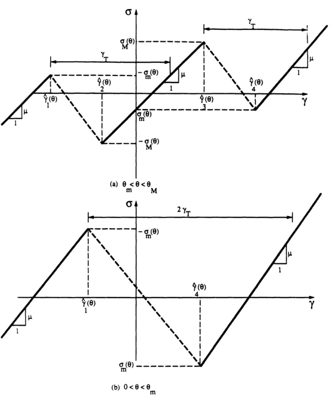
Two graphs of a(y,8) versus are shown in Figure 3.2: Figure 3.2(a) corresponds to a fixed value of temperature in the range O < < M and the stress-strain curve shows three rising branches corresponding to the three phases A, M+ and M-;

Figure 3.2(b) is associated with a temperature in the range 0 < 0 < 0, and the two rising branches of the stress-strain curve correspond to the variants M+ and M-.

Of the three parameters 91, 92 and 93, one is fixed by the choice of reference

configuration, while the other two are determined through the transformation strains.

In particular, if we choose stress-free austenite at the transformation temperature OT to be the reference state, then by setting &(O,OT) = 0 in (3.16)1, one obtains

91= -arT. (3.17)

Next, let 7T(> 0) denote the transformation strain (see Figure 3.2(a)) between each martensitic variant and austenite. Then, from (3.16)

7T = 92 - 91 = 91 - 93 > 0.

(3.18)

(This can be readily generalized to the case where the transformation strain between phases A and M+ is say 7T, and that between A and M- is T$7T.) Finally, if (3.13), (3.15), (3.17) and (3.18) are substituted back into (3.12), one finds that

po(7, 0) contains the term p 1+ (/2)a 242 + pc log(O1l/T) as an inessential linear

function of temperature which may be eliminated by taking

Pi = -(i/2)a 292, 81 = OT- (3.19)

In summary, the material at hand is characterized by the common elastic modu-lus , specific heat at constant strain c and coefficient of thermal expansion a of the phases; the stress-free transformation temperature T; the mass density p in the ref-erence state; the latent heat AT at the temperature T; and the transformation strain

7T. The Helmholtz free-energy function is given by combining (3.12) with (3.13), (3.15), (3.17)-(3.19):

(./2)y2- -la(o - T) + PCo(1 - log(/0T)) on P,

(/2)(y - ) - a( - yT)(O - T) + pcO(1 - 1og(/oT))

pO(7,, ) = - pAT(1 - /T) on P2,

(u/2)(7 + YT)2 _-

_/a(7

_T)

- pAT(1 - /oT) on P3.

The various other thermo-mechanical characteristics of the material can now be de-rived from (3.20). In particular, the stress-response function (7, 0) = p(7, 0) is given by

J

i

-

-OT)

on P

,

a(yf, 0) = I( -T) -a(O - OT)

on

,

1

In order to complete the description of the Helmholtz free-energy function we need to specify the regions P1, P2 and P3 of the (7,0)-plane shown in Figure 3.1, i.e. we need to specify the boundary curves 7 = i(0) shown in the figure. To this

end, we first prescribe the levels at the local maxima and minima of the stress-strain curve. As indicated in Figure 3.2, we take, for simplicity, these stress-levels to be given by ±aM(O) and am(0). In view of our earlier assumption that the boundaries of the regions P1, P2, P3 are straight, the functions uM(O) and (0))

must be linear in . Moreover, since according to Figure 3.1 we must have z2(0,) =

%3(Om), 3(OM) = 4(eM) and i(OeM) = 2(0M), it follows that ~oM(Om) = 0 and

oaM(Om) - am,(OM) = -IT. Thus

aM(O) =

AM(O

-0m)

(3.22)

0m(0) =

m(

-OM) +

lM(eoM-Om)- A7T

<

where m and M are positive material constants. The equations 7 = i(0), i = 1, 2,3, 4,

describing the boundaries of P1, P₂ and P3 are then given by ±oM(O) = &(0), ),

i =

3,

2, and

= a(i(0),o), i

4, 1.

Thus far, we have only described b on the ("metastable") portion P1 + P2+ P3 of

the (, )-plane. It is not necessary, for the purposes of the present chapter, to specify an explicit form for b on the remaining ("unstable") portion of this plane; any func-tion ih which is once continuously differentiable, is such that b., is negative on the

unshaded portion of Figure 3.1, and conforms with (3.12) would be acceptable. An infinite number of such functions exist, provided only that the material parameters satisfy certain inequalities; this is discussed in the appendix.

3.3 Driving force and latent heat

Since stress is uniform throughout the bar, it will often be convenient to utilize expres-sions for the quantities of physical interest in terms of a and 0. Because the relation (3.21) between stress and strain at fixed 0 is not globally invertible, such expressions must be obtained separately for each phase. Inverting (3.21) gives the strains related to the stress through

(, O) =

/h + a( - T)

on P,

2(0,

a)

a(

on P2,

(3.23)

3(0, a) = / + ( - T) -T

on P

,

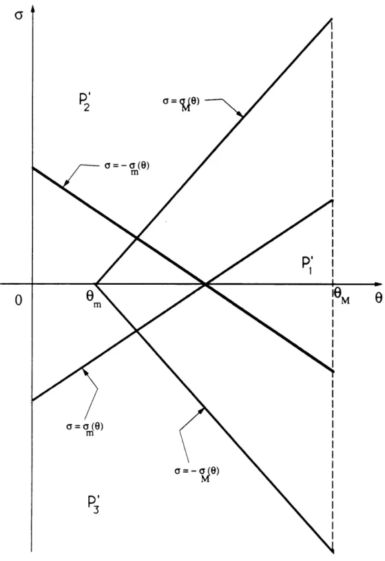
where Pi' is the image of Pi in the (0, a)-plane. Given the stress a and temperature 0 at a particle, Figure 3.3 shows all of the phases that are available to that particle.

The specific entropy is given, according to (2.1), (3.20) and (3.23), by

a/lp + (a 2_{/p)(0 - OT) + clog(0/0T) on P;,}

7

aa/p

/p)(8

(3.24)

au/p + (,ta

/p)(6 - OT)

+ clog(/0T) - AT/OT on P

3

.

The potential energy function G(-y; 0, a) = pOb(y, 0) - y of the material at hand

can be calculated using (3.20). At each (, a), G has one or more local minima. The values of G at the local minima coincide with the Gibbs free energy per unit reference volume. In terms of 0 and a, the Gibbs free-energy per unit reference volume for each phase is obtained by combining (2.3) and (3.23):

9(0, ) =

-(1/2u)[ +

ai(0

-(1/2A)[o + ALa(e

- pAT(1 - 0/0T) - r7T on P2, (3.25)

-(1/2p)[o + tca(O

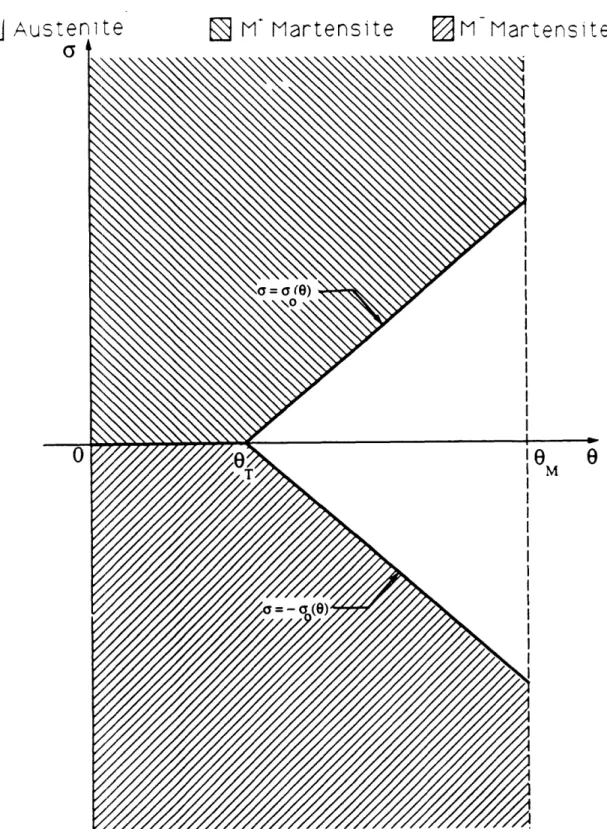
Where G has multiple energy-wells, one can use (3.25) to determine the particular minimum that is smallest. The result of this calculation is displayed in Figure 3.4. The stress-level o0(0) indicated in the figure is given by

ro(0) = pAT 1), (3.26)

7T T

and is known as the Mazwell stress for the A - M+ transition. The Maxwell stress for the A - M- and M+ - M- transitions are -ao(0) and 0 respectively. The two

states A and M+ that are both associated with any particular point on the boundary

a = ao(0) both have the same value of potential energy G and both are stable; if

these states coexist and are separated by a phase boundary, the driving force on that interface would be zero and the phases would be in phase equilibrium.

Suppose momentarily that a particle always chooses the phase that is stable from among all phases available to it. Then the response of a particle as the stress or tem-perature is slowly varied is fully determined by Figure 3.4. For example, consider a fixed temperature 0 greater than the transformation temperature 0

. As the stress

oa is increased monotonically from a sufficiently negative value, the particle is in the martensite variant M- until the stress reaches the value -o(0); it then transforms

to austenite and remains in this phase as the stress increases over the intermediate range -o(O) < a < o(O); at a = ao(O) the particle transforms to M+ and remains there for a > o0(O).

The immediately preceding discussion assumed that a particle is always in the stable phase. In solids however, particles can often remain for long times in states that are merely metastable and the transition from a metastable phase to a stable phase is controlled by additional considerations, viz. nucleation and kinetics. We will discuss these issues in Chapter 4.

We now turn to the driving force on a phase boundary. Suppose = s(t) denote the location at time t of a phase boundary in a bar, and the particle on the left of the phase boundary is in phase-i while the particle on the right is in phase-j (recall that i = 1, 2, 3 corresponds to phases A, M+_{, M- respectively). The driving force}

a from (3.25) and (3.26):

f

= T(L-O(0))

f = -YT(-OCO(O))

7yT(O

ao(e))

f = -YT(a + a(8))

f = 2ayT

f = -

for a M+/A interface,

for an AIM+ interface,

for an A/M- interface,

for a M-/A interface,

for a M

_interface,

for a M-/M

_interface.

The latent heat A = 8( - 77) is the heat generated when a unit mass of material changes phase from (, 9) to (7, ) under conditions of phase equilibrium f = 0. The latent heat for various transitions are calculated from (2.1)2 and (3.20):

8

A

ATA = ATAT

-A = 0

for austenite --, martensite,

for martensite --. austenite,

for martensite ,-, martensite.

Thus when a unit mass of austenite transforms to martensite at the temperature 0 the amount of heat generated is AT(O/OT); in the reverse case the same amount of heat disappears. There is neither heat generation nor disappearance associated with

the martensite -. martensite transition.

Turning next to the heat conduction law (2.11), we take the heat conductivity of the three phases to be the same, and constant:

k(7, 0) = k = constant > 0 on P1,P2 and P3. (3.29) Finally, the positive constants in the heat supply rate (2.12) are given by

c=

P 0C,

pw ¢. = P 0, E,pw (3.30)

where p and w are the circumferential length and cross-sectional area of the bar respectively; qc and b, are the convective and radiation coefficients respectively; E is

the emissivity of the lateral surface of the bar.

(3.27)

Appendix: Restrictions on the material parameters.

Here we shall list all of the inequalities not displayed previously which the material parameters must satisfy. According to the statement below (3.22), the equations of the boundaries of the regions Pi in the (, )-plane are given by

yl(o) = -al - T + (o - T) for 0 < < M,

72(6) = -aM/ + (O- OT) for m < <

M,

73(6) = M//l + a( - T) for 0 < 6 <

0M,

74(0) = m// +

7T

+ o(O - OT)

for 0 < 0 <

_M,

where the stress-levels a,m(8) and arM(G) are given by (3.22). In order that the cor-responding straight lines in the (, 0)-plane be arranged as shown in Figure 3.1, it is necessary that 4(0) > 3(0) > 2(6) > 1(6 ) > -1 for 0m < < and that

74(0) > 1(O) > -1 for 0 < 0 < 0,. These inequalities can be expressed, upon using

(A.1), as

0 < M(O) < om,(0) + IVYT < + a(O - T) for 0, < 0 < OM,

(A.2)

0 < am(8) + 1Y7T < /X + 1a(6 - OT) for 0 < < O6.

Next, since we assumed in Section 3.2 that all three phases M-, A and M+ exist

when a = 0 and 0 = OT, it is necessary that the corresponding strains 7 = -YT, 0

and 7T lie in the appropriate strain ranges as defined by Figure 3.1. In view of (A.1) and (A.2), one finds that this holds if and only if

wT < 1, a(OT) < 0. (A.3)

We turn finally to the issue of extending the Helmholtz free-energy function (3.20) to the unshaded ("unstable") region of the (, )-plane shown in Figure 3.1. Even though we do not need an expression for ,b on this region, it is still necessary to know that (3.20) can be extended to that region in the manner previously assumed (see paragraph below (3.22)). The ability to do this is equivalent to the ability to

connect each adjacent pair of rising branches of the stress-strain curve in Figure 3.2 by a declining branch with prescribed area under it. Since the stress-strain curve is to be declining for strains in the intervals ( 1(e), 7 2(e)) and ( 3(0),'y4(0)) when

8,m < < M, and on (71(8),74(0)) when 0 < < ,, it is necessary that M(O) > am(8) for O, < < OM,

-am(o) >

a,(o)

for 0

< <

o,.

(A.4)

Next, as is readily seen from Figure 3.2(a), for 0,,, < 0 < 8_{OM, the area under the}

graph of a(*, 8) between -y = 13(0) and 7 = 4(0), must necessarily lie between the areas of the two rectangles with the same base ( 3(0),1 4(0)) and with heights aM(e)

and am(0). A similar restriction applies to the area between 7 = 1() and 7 = /2(0),

and for 0 < <

e,

that

-aM(O)(72(O)- 1()) < p(5 2(),)-p(l((),G) < -m(e)(5 2()-1(0))

am(o)(j4(e) - 3

())

0m(0)(74(O)

-

,())

-am(o)(4()-1(0)),

holds for 0 < < Om. Conversely, given two points (3(0), M(8)) and ( 4(0), am(@))

in the (, a)-plane, with 4(8) > 3(0), a sufficient condition for the existence of a

continuous decreasing function &(., 0) connecting these two points, which is such that the area under it is p(4(0),

8)

requirements (A.2), (A.5) are therefore necessary and sufficient for the extendability of the Helmholtz free-energy function (3.20) to the unstable region.

The inequalities (A.5) can be expressed equivalently in terms of the stresses a,,(),

TM(O) and ao(O) as

[aM(0) - am(O)]2 < 27T [ao(8) - m(O)] for Om < < OM,

[aM() - am(O)]2 _{< 27T [M() - (0)] for}

_Om

_OM,

The inequalities (A.2) - (A.4) and (A.6) must be enforced on the material model. They can be reduced by using (3.22) and (3.26) into temperature independent in-equalities that involve only the material parameters. We shall not display the result-ing inequalities here. These inequalities, as well as one more restriction like (4.2), are to be imposed on the material constants entering into our model.

One can verify that the particular values (5.6) of the material constants, together with a range of values of the four remaining parameters m, M, m and M, do satisfy these inequalities. For example, one possible set of values of the latter four parameters are m = 9.7253 x 10-5 / °K, M = 10.1371 x 10- 5 / °K, 0,m = 285 OK, OM = 10000 K;

as mentioned previously, the particular values of these four material constants does

I I I I A il, l i ^ P1 A Y (0) 3 -1 0 Y

Figure 3.1: Regions P1, P2 and P3 in the (7, 8)-plane.

a

-

¥

Figure 3.2: Stress-strain curves at constant temperatures .

TT r~~~~~~~~~~~~~~~~~~~~~~~~~~~~ 1 M I I I I I I I I I I I I I I w

Figure 3.3: Available phases at a given (, a).

0

a

I

Figure 3.4: The stable phases.

FM

m

a t ns

t

e

Chapter 4

Nucleation Criterion and Kinetics

4.1 Nucleation criterion

The instant of time at which a new phase is nucleated, the number of associated phase boundaries and their spatial distribution are determined by a nucleation criterion. In this thesis we shall often encounter quasi-static processes in which the entire bar is in a single phase for an initial interval of time and in two-phase states for subsequent times. The criterion that determines the instant of initial nucleation we refer to as

the initiation criterion.

First we discuss the initiation criterion. We suppose that a particle which is in phase-i will transform to phase-j by nucleation if the driving force f at the incipient phase boundary would be at least as great as a certain materially-determined critical

value: f > fij; the associated initiation criterion is thus given by setting f(O, a) = fj

in (3.27). For simplicity, and in view of symmetry of the potential energy function

G when = 0, we shall assume that both the A -, M+ and A - M- transitions

initiate at the same value of temperature if the stress vanishes; a similar assumption for the reverse M+ -- A and M- -- A transitions will also be made. The former

value of initiation temperature is denoted by M, (for "martensite start") while the latter is denoted by A, (for "austenite start"). We will also assume that at any given

temperature 0, the initiation stress-level for the M+ - M- transition is the negative of the initiation stress-level for the M- - M+ transformation at that temperature.

this leads to the following initiation criteria for the various transitions:

- ao(0) -o(M.)

for A

M

,

a - o() < -aoo(A.)

for M

A,

a + ,o() < o(M.)

for A

M-,

a + o(0) < ao(A.) for M- A, (4.1)

a >

for M-

M

_,

< -

for M

_,

where uo(0) is the austenite-M+ martensite Maxwell stress given by (3.26) and the constants M,, A, and E are characteristic of the material.

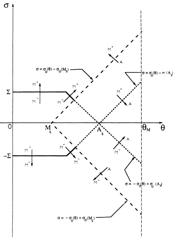
Figure 4.1 illustrates these initiation criteria on the (, a)-plane. If the inequalities in (4.1) hold with equality, the resulting equations describe a set of straight-lines in the (0, a)-plane; the initiation criterion states that, as indicated in the figure, crossing one of these lines initiates an associated transition. Figure 4.1, as shown, corresponds to a material for which the critical initiation stress-level given by (4.1) for the M- - A transition exceeds the corresponding stress-level for the A -- M+ transition for some range of temperature, i.e.

E

this need not necessarily be the case.

We now turn to the subject of where, when and how many phase boundaries are nucleated, i.e. nucleation criterion. If the current state of the bar were to involve either a temperature or stress gradient, one can determine the location in the bar at which the first nucleation occurs. In this thesis we will consider a uniform bar that is always subjected to uniform stress. When the temperature field is also uniform along the bar as in Chapter 5, the location of the nucleation site in this bar is undetermined and arbitrary. In this case we assume that the transition from a low-strain phase to a high-strain phase would necessarily commence at the left end of the bar and the reverse transition would occur at the right end. If the temperature field is nonuni-form, which is the case in Chapter 6, then the transition from a low-strain phase to a high-strain phase will initiate at the coolest point in the bar, whereas the reverse