Construction of nonlinear filter algorithms using the saddlepoint approximation

Construction of Nonlinear Filter Algorithms Using the

Saddlepoint Approximation

by

Esosa 0. Amayo

Bachelor of Science, Electrical Science and Engineering

Submitted to the Department of Electrical Engineering and Computer Science

in Partial Fulfillment of the Requirements for the Degree of

Master of Engineering in Electrical Engineering and Computer Science at the Massachusetts Institute of Technology

Ccspight 2006 M.T

The author hereby grants to M.I.T. permission to reproduce and distribute publicly paper and electronic copies of this thesis

and to grant others the right to do so.

Author

Department of Electrical Engineering and Computer Science July 18, 2006 Certified by_ Emery N. Brown Thesis Supervisor Certified by_ John L. Wyatt Thesis Co-Supervisor Accepted by_ Arthur C. Smith

SI.ndirmlldn, o-pa LLIImL ,0mmittee on Graduate Studies

Construction of Nonlinear Filter Algorithms Using the Saddlepoint Approximation

by

Esosa 0. Amayo

Submitted to the Department of Electrical Engineering and Computer Science July 18, 2005

in Partial Fulfillment of the Requirements for the Degree of

Master of Engineering in Electrical Engineering and Computer Science at the Massachusetts Institute of Technology

ABSTRACT

In this thesis we propose the use of the saddlepoint method to construct nonlinear filtering algorithms. To our knowledge, while the saddlepoint approximation has been used very successfully in the statistics literature (as an example the saddlepoint method provides a simple, highly accurate approximation to the density of the maximum

likelihood estimator of a non-random parameter given a set of measurements), its potential for use in the dynamic setting of the nonlinear filtering problem has yet to be realized. This is probably because the assumptions on the form of the integrand that is typical in the asymptotic analysis literature do not necessarily hold in the filtering context. We show that the assumptions typical in asymptotic analysis (and which are directly applicable in statistical inference since the statistics applications usually involve estimating the density of a function of a sequence of random variables) can be modified in a way that is still relevant in the nonlinear filtering context while still preserving a property of the saddlepoint approximation that has made it very useful in statistical inference, namely, that the shape of the desired density is accurately approximated. As a result, the approximation can be used to calculate estimates of the mean and

confidence intervals and also serves as an excellent choice of proposal density for particle filtering. We will show how to construct filtering algorithms based on the saddle point approximation.

Thesis Supervisor: Emery Brown Thesis Co-Supervisor: John Wyatt

Acknowledgements

I would like to thank my advisor, Professor Emery Brown for being such an inspiring role model as a researcher. I am deeply grateful for his patience with me and constant support through some very difficult personal trials. In some sense, this thesis would not have happened had Professor John Wyatt not been such a clear and inspiring teacher when I took 6.432 with him. This thesis is the result of my interest in estimation problems that was sparked by that class. I am also greatly indebted to him for his friendship, constant support, encouragement and invaluable advice. Words are inadequate to express my gratitude to Professor Tayo Akinwande who has been a source of inspiration, and above all a father to me since I first arrived here as an undergraduate. My graduate student life would have been stillborn had it not been for the financial support from Dean Isaac Colbert that saved me when I could not initially get funding. I would also like to express my thanks to Dr Chris Oriakhi at Hewlett-Packard Research, whose achievements helped motivate and spur me on and whose friendship and advice helped me through a difficult time.

This thesis would not have been possible without the support and understanding of my colleagues at Aware, in particular my manager Dr Michael Lund and the head of our Engineering division, Dr Rick Gross.

My thanks also go out to Anne Hunter, Vera Sayzew and all the good folks at the course 6 Undergraduate Office for their patience (which I have tested on several occasions over the years and found to be truly limitless) and willingness to go above and beyond the call of duty to help students. I cannot thank Cheryl Charles enough for her kindness, motherly concern and support. I would also like to thank Carol Frederick, my first boss at MIT, for all her support and friendship.

To Dr Jack Lloyd, thank you.

To Stanislav Funiak, Yogishwar Maharaj, Mamat Kaimudeen, Emilia Simeonova, Elana Wang, Cang Kim Truong, Buddhika Khottachi, Felecia Caic, Senkodan Thevendran, Eric Escobar Cabrera, Fitih Mustafa Mohammed, Nathaniel Choge, Ming Zhang, Riyaz Bachani, Bill Blackwell, Pia Bhanerjee, Abhinav Kumar, Bosun Adeoti, Paul Njoroge, Kwaku Owusu Abrokwah, Nii Lartey Dodoo and all my friends I say "thanks Bushtis" for making my life bearable.

I would like to thank my lab buddies, Chris Long, Patrick Purdon, Uri Eden, Somangshu Mukherji, Mike Prerau, Supratim Saha, Riccardo Barbieri, Murat Okatan, Tyler Gibson, and Julie Scott for always being there to talk about anything even at the busiest of times. I spent countless hours talking with Ram Srinivasan about my thesis, and about life outside of the thesis and each conversation left me with renewed encouragement and energy.

To my sister, Dr Ruth Uwaifo, I say "thank you" from the bottom of my heart for the constant prayers and support by letters while you were in Nigeria and by phone when you moved over here.

To my brothers Muyiwa Olubuyide, Jitin Asnaani, and Premraj Janardanan, I say "thank you" from the bottom of my heart for being there and for enriching my life. Your friendship has made me a better person.

Last but definitely not least, I want to thank my mother and sister who refused to be deterred by little nuisances like the Atlantic Ocean in making me feel their love even here.

Contents

A cknow ledge m e nts ... 0 3 Chapter 1: Introduction

1.1 The nonlinear filtering problem... 06 1.2 Brief summary of current approaches ... 08 1.3 Objectives and contributions of the thesis... 08 Chapter II: Summary of Current Practical Solutions to the Filtering Problem

2.1 Linear Least-Squares Estimation ... 10 2.2 The Extended kalman filter... 12

2 .3 P a rtic le filte ring ... 13 Chapter III: Saddlepoint (or Laplace) Approximation -Theory

3.1 The Laplace method for approximating integrals - existing theory ... 17 3.2 New results based on the Laplace method for approximating integrals ... 26 3.3 Proofs of new results based on the Laplace method for approximating

in te g ra ls ... 3 2

Chapter IV: Construction of a Saddlepoint Filter for a Stochastic Point Process Model

4.1 Description of the State-Space Model... 40 4.2 Saddlepoint Filter for the State-Space Model ... 43 4 .3 A p p lica tio n s ... 4 7 Chapter V: Conclusions and Future Directions

5.1 Summary of thesis results ... 61 5.2 Ongoing and future research... 61 Appendix A: MATLAB Code ... 63 R e fe re n ce s ... 7 5

Chapter 1

Introduction

1.1 The Nonlinear Filtering Problem

Our goal is to sequentially estimate the states of a discrete-time system that has nonlinearities in the state and/or the observation process and whose state and/or observation noise processes are not necessarily Gaussian. We will be working with systems that can be described by the following general state space model

Xn, ~ q9xn in-1) yn - r(yn xn)

where y, is an observation from the system, xn is the unknown state process, _q(xn lxn_.) is the conditional distribution of x, given x-,_ and r(yn xn) is the conditional distribution of y, given x,. The initial state is distributed according to the distribution p(xo Y). We assume that the states follow a first order Markov process. That is

A~x jk -1_,,xk_2 x, , o) =9 q k jk-1) 12

We also assume that the observations are independent given the states. That is

P(yk xkyl,y....,y) = r(yk xk) if k>l>m> ... >s (1.3)

The nonlinear filtering problem is to evaluate p(xk fY), the distribution of the current state

given the observations up to the present time Y = {y,...,Yk} and the initial distribution of

the state process. Once we have the filtering density we can calculate a variety of estimates of the state such as the mean (which is the minimum mean squared error estimate of the state), the mode, the median, confidence intervals and so on.

The general state space model considered above includes various important models such as:

(i) The linear state space model with Gaussian or non-Gaussian white noises w, and

x, = Fxn + Gw, _(1.4)

yn =Hx,+En

(ii) The nonlinear model with additive noise

x, = f(x_1

)+w

yn = h(xn)+e,

(iii) _{The more general nonlinear model with known input un}

xn =

f(x_,_,

Yn = h(xn, n9En)

(iv) Discrete Process with probabilistic description of observation process parameterized by the state (for example state space system with point process observations)

xn=Fx + Gwn

(1.7)

yn~ Dist(xj)

1.1.1 Recursive Formulae for Filtering

Using only the definition of conditional probability, the Chapman-Kolmogorov equation for marginal distributions, Bayes' law, and the Markov assumptions mentioned in the preceding section we obtain recursive formulae for the one step ahead prediction and filtering densities as follows:

One step ahead prediction density:

PXk

Y,-)

Filtering density:

P(Xk r(yk Xk)P(Xk - (19)

P(yk lk-1)

where P(Yk Y,) is calculated from

P(yk k-1) = fr(yk Xk)P(Xk l-1)dxk

(1.10)

1.2 Brief Summary of Current Approaches to the Nonlinear Filtering Problem If the state and observation equations are linear and initial state as well as the system and observation noise processes are Gaussian, the system of equations (1.8)-(1.9) has an exact Gaussian solution and the means and covariances of the one-step and filtering densities are given by the well-known Kalman Filter recursion. However in the general not-necessarily-Gaussian case these densities have to be approximated. The most commonly used practical approaches to this problem are the Extended Kalman Filter (EKF), the Unscented Kalman Filter (UKF), methods relying on Gaussian approximations to the left hand sides of (1.8) and (1.9), perfect Monte Carlo simulation (when it is

possible to sample directly from the true posterior density) and particle filtering (which is used when it is not possible to sample directly from the true posterior distribution). We will outline the salient points of some of these methods in the next chapter.

1.3 Objectives and Contributions of the Thesis

In this thesis we propose the use of the saddlepoint method to construct nonlinear filtering algorithms. To our knowledge, while the saddlepoint approximation has been used very

successfully in the statistics literature (as an example the saddlepoint method provides a simple, highly accurate approximation to the density of the maximum likelihood estimator of a non-random parameter given a set of measurements [Barndorff-Nielsen, 1983]), its potential for use in the dynamic setting of the nonlinear filtering problem has yet to be realized. This is probably because the assumptions on the form of the integrand that is typical in the asymptotic analysis literature (for example [De Bruijn, 1981]) do not necessarily hold in the filtering context.

In the sequel we will develop filtering algorithms based on the saddle point approximation. This gives us an approximation whose shape accurately approximates the shape of the target density. As a result, the approximation can be used to calculate estimates of the mean and confidence intervals and also serves as an excellent choice of proposal density for particle filtering.

In Chapter 2 we will discuss the most common approaches to the nonlinear filtering problem. We will then discuss the existing theory for approximating asymptotic integrals using the Laplace method (the analogue of the Saddlepoint method on the real line) and then develop some new results with modified assumptions that can be used to approximate probability densities that can not necessarily expressed as the integral of a function which is the exponential of a well-behaved function scaled by a large constant. We will then show in Chapter 4 how the results obtained in Chapter 3 can be used to construct filtering algorithms.

Chapter 2

Summary of Current Approaches To The Filtering Problem

In this chapter we will first describe the well-known Kalman Filter solution to the linear estimation problem. We will then outline some of the methods currently being used to deal with the more general non-linear estimation problem such as the Extended Kalman

Filter (EKF), which is based on the Kalman Filter and Sequential Monte Carlo (Particle Filtering) methods.

2.1 Linear Least-Squares Estimation

In this section we will summarize the Kalman Filter solution for obtaining the linear minimum mean-squared error estimate of a random process x, from measurements yn. Our treatment will closely follow that of [Luenberger, 1969, Chapter 4].

The random process x, is assumed to evolve according to a vector difference equation

xn = Fx + W, n = 0, 1, 2,..., (2.1)

where x is an n-dimensional random vector, F is a known nxn matrix and w, is an

n-dimensional random vector input with mean zero satisfying E[w(k)w'(l)] = Qk3

kl (in other

words, the random vector input is "white"). The initial random vector is assumed to have mean kc and covariance matrix P.

Measurements of the process are assumed to be of the form

y = Hnx + En, n = 0, 1, 2,..., (2.2)

where H is a known mxn matrix and e is an m-dimensional random measurement

other words, not only is the measurement error "white", no component of each measurement error vector is a deterministic affine combination of the other components) .

The above state-space model is actually motivated by current understanding of the physical properties underlying most real-world systems. It is believed that basic randomness at the microscopic scale including electron emissions, molecular gas velocities, and elementary particle fission are basically uncorrelated processes. When their effects are observed at the macroscopic scale with, for example, a voltmeter, we obtain some average of the past microscopic effects [Luenberger, 1969].

The linear least-squares estimation problem is most conveniently tackled by formulating it as an equivalent minimum norm problem in the Hilbert space of random vectors with finite second moments [Luenberger, 1969] [Kailath et al, 2000] and inner product (u,v) = E[uv'] where u,v are elements of the Hilbert space. The optimal estimate of x,, given the observations up to time n , which we will henceforth refer to as xn1n ,is the projection of xn

onto the space spanned by the random vectors yo , yl, ... , yn. The recursive Kalman filter solution is obtained as follows.

First, we assume that we have measured yo, y₁, ..., y,_1. and that the optimal one-step

estimate, & _1 which is the projection of x onto the space spanned by the random

vectors yo , y1, ..., yn, 1, together with the error covariance matrix

PIn_, = E[(x_1 -xn)(xn_1 - xn)'], have been computed. The updated estimate can then be shown to be [Luenberger, 1969] [Kailath et al, 2000]

_ +PH'[HP _H'+R1 ]-1[y

Hi2

]

with associated error covariance

Xn+1n = FnXil (2.5)

with error covariance matrix

Pn+11n = FPntnF'+Qn (2.6)

The above Kalman Filter solution to the linear least-squares estimation problem does not assume that the input and measurement error processes are Gaussian and requires only knowledge of the means, variances and covariances. However, when the input and measurement error processes are Gaussian, the Kalman filter solution is also the solution to the general optimal minimum mean-squared error estimation problem. In other words, the Kalman filter recursions provide the mean and covariance matrix of the Gaussian

posterior density at each time step [Luenberger, 1969] [Kailath et al, 2000].

2.2 Approximate Nonlinear Filtering Using the Extended Kalman Filter

Since most practical systems are nonlinear, a lot of effort has been put into developing approximate nonlinear estimation algorithms. One of the earliest methods developed is the Extended Kalman Filter (EKF), which is based on a linearization of the state and measurement equations of the nonlinear state-space model. As an illustration of the general idea, consider the model given below.

xn

f,_

yn =hk (x,)+ en (2.8)

Let _ be the estimate of xn given the measurements yo , y1, ... , y,_,. Replacing

f_,(x-,_) and hn1(x,_,) above with the first order terms from their respective Taylor series

expansions about ^i, and then applying the Kalman filter algorithm to the resulting linearized system then results in the Extended Kalman filter algorithm for the state-space

model. This algorithm is given below [Kailath et al, 2000]. In the algorithm below Rk , QA , ZnIn, Anin- , 'i Pnjn are specific to the linearized system and all have the same

meanings as in the previous section.

= +P H' [H H+ -H

]

(~

Unfortunately, there are almost no useful analytical results on the performance of the EKF. A considerable amount of experimentation and adjustment is needed to get a reasonable working filter [Kailath et al, 2000].

2.3 Sequential MonteCarlo (Particle Filtering)

Importance Sampling

In perfect MonteCarlo Simulation the mean of any function of the state process at a given time conditional on the observations up to that time can approximated by a weighted sum of samples drawn from the posterior distribution. The law of large numbers then guarantees that the accuracy of this approximation will increase as the number of samples drawn increases. Unfortunately, it is often impossible to sample from the posterior density. This difficulty can be overcome by drawing samples from a known function that is easy to sample as will be illustrated below.

Let X = {xO,..., Xk} and Yk = {Y,.'Yk} be the states and observations up to the present

time and let s(Xk IYk) be the proposal density that is easy to sample from. We will show

below how samples from the proposal distribution can be used to approximate the mean

of a function g(X) .The mean of g(Xk) is given below:

E[gk(X)]= fgk(Xk)p(Xk Y)dXk

(2.13)

The mean can be re-expressed in terms of the proposal distribution as follows (see [van

der Merwe, 2000] for more details)

E[g (Xk)]

f

Wk(Xk)S(Xk IY)dXk

where the weight

is given by

Wk(Xk) = P Xk)p(Xk) (2.15)

s(Xk

4)

In (2.4) above, the mean of the function has been re-expressed as a ratio of means, each

taken with respect to the proposal density. Hence by drawing samples, Xk"' = {xf4,..., x} ,

from the proposal distribution we can approximate the expectation in (2.13) above by the

following

N

(2.16)

The estimate in (2.16 above is biased as it involves a ratio of estimates. However, if the conditions below hold:

1. X)" is a set of independent and identically distributed samples drawn from the proposal distribution, the support of the proposal density includes the support of the posterior density and the desired mean in (2.13) exists and is finite

2. The weights wk(Xk) and the variance of g,(X,) are bounded

the estimate in (2.16) will converge asymptotically to the true mean [van der Merwe, 2000].

Sequential Importance Sampling

The result in (2.16) does not lend itself to the sequential estimation of the mean as new observations are received. In order to compute a sequential estimate at a given time without having to modify the previously simulated states, proposal distributions of the following form can be used:

s(Xk Y) = S(Xkl _ 1k_)S(Xk Xki _Y) (2.17)

Under our assumptions in the previous chapter that the states correspond to a Markov process and that the observations are conditionally independent of given the states, we get the following:

j=k p(Xk) =

P(X

)H(x

Wk -: Wk__

r(yk xkl)_x)q(xk

s(xk ,Xk,)

(2.19)

Hence, given an appropriate choice of s(xk Xk,,Y) the importance weights can be updated sequentially and hence estimate of the mean given in (2.16) can also be updated sequentially as illustrated in the algorithm below:

1. Initialization: set k =0 and for i=1,...,M

p(x0 IY) and set wo) = M-1 for all i.

Set k=1

particles, draw the initial states xO" from

2. Importance Sampling: For i=1,...,M, draw ik{" from sk(Xk XkY,1)

acceptance/rejection algorithm and set 4: - ( 0) Evaluate the importance

weights:

Wk k = Wk_k

Sk (Xk Xk ,Yk)

and then normalize them:

M

j =1

3. Update Mean and Variance: Compute the marginal conditional mean and variance as follows: M xkk = M-1 W(x i=1 Wkk =M-1((x (i)'-xkxk) i=1 X k using the

Chapter 3

Saddle Point Approximation: Theory

We will first discuss how the Laplace method can be used to approximate asymptotic integrals with vanishingly small approximation error. Unfortunately the assumptions on the form of the integrand may not necessarily apply in the nonlinear filtering context. Using a method analogous to the Laplace method for asymptotic integrals, we obtain bounds on the integral and approximation error for the integrals of what we will refer to as exponentially concentrated functions. These results can then be applied in understanding the error performance when the Laplace approximation is used in the nonlinear filtering context.

3.1 The Laplace Method for Approximating Integrals

We will focus our attention on integrals over real intervals where both the integration interval and the integrand may depend on some parameter t, as illustrated in Equation 3.1 below. The Laplace method is usually used to investigate the asymptotic behavior of such integrals as t -+ oo.

F=

Jg(x,

In this section we will first present a heuristic argument for determining the functional form of the Laplace approximation for a very general case. Finally we will formally state and

prove the result. The proof will follow the outline provided in [DeBruijn, 1981 Ch.4] while filling in details omitted in that text.

Heuristic Derivation of the Laplace Approximation

The key idea behind the Laplace method is that if there is an interval I such that the integral over the complement of that interval is small compared to the integral over I, we can then try to approximate the integrand by simpler functions throughout I. To make this a little more specific we will consider integrals of the form:

F= Jexp{th(x)}dx . (3.2)

where t is a positive real constant and h(x) is a real continuous function. Furthermore, we will assume that h(x) has a unique global maximum at the point x = x0 and that its first

and second derivatives exist in some interval. Since h(x) has a unique global maximum at the point x0, the value of the integral for large values of t will be dominated by the

behavior of h(x) near its maximum. Therefore there will be a small interval I around the maximum such that the integral of exp{th(x)} over the complement of I is small compared to the integral over I.

Further assume that the Taylor's series expansion of h(x) about the point x converges in I:

h(x) = h(xo) +h'(xo)(x - x0)+Ih"(x0)(x -X0 )2 + higher order terms (3.3)

2

Since h(xo) is a global maximum, h'(xo) = 0. Therefore h(x) may be approximated by simpler functions as

12

h(x) h(x)=h(xo)+-h"(x0)(x-x0)2 , for xe I (3.4)

Since

fJ-J

is small compared to

exptth(x)}dx

we can approximate the

integral in (3.2) by the integral over I, which in turn can be approximated by the integral

of the simpler function over I. This integral is then approximated by the integral over the

entire interval (which is easily evaluated) yielding the Laplace approximation. These steps

are illustrated below:

f exp{th(x)}dx

=

exp{th(x)}dx

exp{th(x)+ 2 x{th" (xo))2}d x

= expjth(xO)} exp{ th",(xo)(X-_XO)2}Idx

= (2rr)2 (-th"(xO)) exp{th(x,)}

So the Laplace approximation to the integral in (3.2) is

F(t)

)}

Rigorous Statement and Proof of the Result

In this section we will establish bounds on the integral in (3.2). Before we state the proof

of the main result we will prove a lemma that will be used in the proof.

Lemma 3.1 Let h(x) be a real and continuous function. If

ii. h'(x) exists in some neighborhood of x0, h"(xo) exists and h"(xo)< 0

Then, given positive e, we can determine 6 0 such that

h(x) -h(xo)- 1(xxo)2h"(xo) E(x-x 0)2 ,for x-xo0

1

Proof Let qp(x) = h(x) - h(xo) -(x - xO)2 h"(xO). Since h(x) is maximal at x = x we infer

2

that h'(xo) = 0. Consequently q'(xo) = p'(xo) = O'(xo) = 0. p"(xo) = 0 implies

(x - xo)-'('(x) - p'(xo)) -> 0 when x -> xO. Since _{P'(xo) = 0} this means that qp'(x) = o(x - xO) ,(x -+ xO). Applying the mean value theorem [Rudin, 1976 Theorem 5.5] to ((x) we see that q(x)-q(xo)=(x-xo)-''(xo+6(x-xo)) for some 0<0<1. So

P(x) = (x -xO)o(9(x -x)) = o((x -x)2) ,(x -> x0). Since V(x)=o((x-xO)

2_{), for a given} positive e we can find 6 0 such that q'(x)! e(x-xO)5 2 _{for jx-x j 6 ,5 which proves the}

lemma.

We will now state the main result below.

Theorem 3.2 (Bounds on the Integral) Let F(t)= Jexp{th(x)}dx, where h(x) is a real

and continuous function and t 1. If

i. h(x) has a unique global maximum H. at x = xO

ii. there exist numbers A < H. and a such that h(x) A if

|x

iv. h'(x) exists in some neighborhood of x0, h"(xo) exists and h"(xo)< 0

Then for any e such that 0 < 3e < h"(xO)|, there exists a positive real number T such that for t T the following inequality holds:

1 1 1 1 1

eth(xo)(2/T)i(-h"(xO)+3e) t-2 <F(t) < eth(xo)(2,r) (-h"(xo) -3e) it 2

Since e is arbitrary, for sufficiently large t we have the following Laplace approximation:

1 1

F(t)~ F(t) =(2ff)2 (-th"(x0)) 2exp{th(x0)}

Proof Applying Lemma 3.1 we see that for any positive e we can find 6 0 such that for ix-xoj0 5 the following inequality holds:

h(x)-h(x

I

Therefore the following inequalities hold:

S(x-xo )2t(h"(x0)-2e) xo-d5 xo+3X x+8 xO +'5 thx-6o) x0 2 (X )2t(hN(x)+2e) t(h(x)-h(xdx < dx xO-,5 _xO-6

As the integrals over (-oo,oo) of the leftmost and rightmost integrands will be used later in the proof to establish bounds on F(t), we will limit our choice of e to the range

0<3e<jh"(xO)j. This will ensure that the exponent of the integrand in the rightmost

integral in (3.6) is negative.

Let D1, D2 and D3 be the amounts by which the integrals above differ from the corresponding integrals over (-oo,oo). That is:

K

06

0

S(x-xo)21(h(xo)+2e)dx

ef(X-XO)2t(h"(xo)-2e)dx

Adding D + D2 to both sides of the inequality on the right and D, +D3 to both sides of the inequality on the left in (3.6) above we get the following inequalities for the integrals over (-oooo):

e(x-xO)2t(h"(x)-2v dx+D, -D 3 <e-th(xO)F(t)< fe o2t(h(x0)+2) dx+D, -D 2 (3.7)

S 11 1

Since fJe 2 Xo\\ dx =(2ir) 2 (-h'(x₀) T 2E) 2t2 the inequalities in (3.7) become:

(27r)(-h"(xo)+2e) t

+D

1 11

e-th(x)F(t)<(2r)2(-h"(xo) -2e) 2_{t 2+D -D}

2 (3.9)

We will now establish bounds on D,, D2 and D3. It follows from our assumptions that for any 8 !0 there exists a positive number q1() such that h(x)-h(xO) -q(8) when

x-xoj 8i. If 45 a then assumption (ii) in the statement of Theorem 3.2 implies that q₁ (8) = Hma - A. If 5 a, let B be the maximum of the continuous function h(x) in the interval 8 ix - x0 I a. B>A then implies that q()= Hm - B otherwise

71(8) = Hm - A.

Rewriting t[h(x)-h(xo)] as t[h(x)-h(x0)]=(t-1)[h(x)-h(x0)]+[h(x)-h(x0)] and applying

the inequality h(x) -h(xO) -i7 (8) to the second term on the right hand side we get the

following inequality:

t(h(x)-h(xo)) -(t -1)i7(S)+h(x)-h(x) for t >1.

exp {-(t

1)q7 (6)

h(x)

h(xo)}dx

5 fexp{-(t

Therefore

D, K, exp{-tq1(6)} where K, = exp1,7(J)- h(xo)} fexp{h(x)}dx.

The functions -(x- xO) 2 t(h"(x0)

2 + 2e) and

1(x _{- xo)2t(h"(xo) - 2e)}

2 each have a unique

global maximum value of 0 at x = x0. Furthermore, since the constants t(h"(xo)+ 2e) and

t(h"(xo) - 2e) are both negative, the functions are both monotonically decreasing for

Ix- xo>0 and exp[ (x -xO) 2 _{t(h"(xo)±2e)] is a Gaussian function and hence its integral}

2

exists. As a result we see that these functions satisfy the same assumptions (i)-(iii) which we made on h(x). Hence we can establish the following bounds for D2 and D3 using the

same argument we used above for D,:

D2 K2exp{-tq2(3)} where K2 = exp J2()j exp11 (X-Xo)2(h"(xo)+2e)}dx

772 = g2(-h"(xo)-2e)

12)2

D3 K3exp{-tq3(3)} where K3= exp1 3(9)1 exp o)2(h"(xo)2e)}dx

7721)= 52(-h"(xo)+2e)

2

Since DI, D2 and D3 are positive, the following inequalities hold:

and

and

D1 -D2 < D1: K1exp{-t 1(9)}

D -D 3 > -D3 > -K 3exp {-t 3(8)}

Plugging the above inequalities into (3.8) and (3.9) we get the following inequalities:

(2r)2 (-h"(xo) + 2e) 2_{t 2 - K} 3 exp {-tU3 (6) 1 1 1 e-th(xo)F(t)

<(2ic)

_(-h"(x

)--2e)

(6)}

will decay much faster than the difference between

1 1 1

and (2fT) 2_{(-h"(xo) +}

3e) 2t 2 (which decays

1 s1 1

when

I I

(2z)2 _{(-h"(xo) + 3C) 21}

1

(2,)2(h (O)+ 3e)

will be greater than

.This together with (3.1) implies that:

2t <e--th(xo)F(t) (3.12)

Similarly, as t increases K exp{-tq1(i5)} will decay much faster than the difference

1 1 1

between (2,T)2(-h'(xo)-3C) 2

t 2 and

Therefore when t is sufficiently large

1 1 1 1 (2;r)2(-h"(xo)-2e) 2 t 2 (which decays as t 2). (2T)2 (-h"(xo)-2e) 2 t 2 +K, exp{-t ₁(6)} will be I 1 1

less than (2;) 2_{(-h"(xo) -3E)} 2

t .This together with (3.11) implies that:

e-th(xo)F(t) <(2'r)2 (-h"(xo) - 3E) 2 2

and completes the proof.

(3.10)

(3.11)

as t 2). Therefore

Theorem 3.3 (Direct Evaluation of the Laplace Approximation Error) F(t) = F(t) + Kt-1 for some positive constant K.

Proof

The Taylor's series expansion of h(x) about the point x0 is given by:

h(x)=h(xo)- (x -xO) 2+ 1H 3 (x-xO)3+ - H 4(x-xO)4 +higher order terms

22 6 24

where, .2 - , and Hk = (d/dx)k h(x) .The integral can then be expressed as

th(x)dx=eth(xo)f 2 1 (X-X₀)2 retHk (x--x₀)kdx

feth~x~x = e f 2t-la k>3 i d

Expanding each term of the form H in its Taylor series

get the following:

(x x)k k>3 expansion about 0 we 2 3 + 2.(k !)2 H

(Xx)

6.(k

for some constants Ak . Since integrals of the form f(x-xO)ke 2(O) dx equal zero for odd numbered integers k, only the even powers in the sum above contribute to the integral in (3.14). Therefore we have the following

Jeth(x)dx = eth(x0)

I f -XOa 2 d+ Jx ) e2 1

fe~ 2 (X-- dx+ I A2, -( X _X( 2k e-2-a(-

dx

k>2

Using known results on the central moments of Gaussian distributions to evaluate the first few integrals in the sum above yields the following result (see the appendix of [Tierney and Kadane, 1986]):

(3.14)

eth(x)dx=(2ffo-t )=eth(xo) I+BIt-1 +B2t-2 + (t-3)

where

B, =-07'H, +-5 yH 2

8 24

B=I07H

48 384 48 64 1152

3.2 New Results Based on the Laplace Method for Approximating

Integrals

Laplace Approximation for Exponentially Concentrated Functions

In the previous section we presented a heuristic argument to derive the Laplace

approximation for integrals of functions of the form

exp{th(x)}

for large positive real

values of t (which must be greater than 1) and a properly behaved function

h(x).

Our

eventual goal is to apply this method in approximating the one-step update integral in the

BCK equations for the general filtering problem given in (1.8). Unfortunately, the

integrands of interest in the general filtering problem cannot necessarily be expressed in

the form exp{th(x)}.

An obvious first step towards our eventual goal would be to examine approximations to

integrals of the following form

We could apply a similar heuristic argument as the one used at the beginning of the previous section to arrive at the following approximation:

F

=

2(-h"(x))2exp{h(x)}

However, the results establishing bounds on the integral and asymptotic error performance of the approximation presented in the previous section will not necessarily hold. In order to use the approximation in (3.15) to construct nonlinear filtering algorithms it is essential to have a good intuitive understanding of how the behavior of the integrand will affect the error performance of the approximation in (3.15).

By focusing on the integrals of functions which have the following properties (we will refer to such functions as being exponentially concentrated)

* existence of a unique global maximum

" the integral of the function over the complement of a neighborhood of the maximum decays exponentially as the radius of the neighborhood increases bounds on the approximation in (3.15) can be established using a method analogous to that used in the proof of Theorem 3.2. In particular, we show that for exponentially concentrated functions, the following bound on the integral holds (see the proof of Theorem 3.5 in the next section for more details and a more rigorous statement)

1 -1 1 1

(2f)2 (-h"(xO) + 2e)2 - K₂(t)e-' < e-h(xo)F <(2f) 2 (-h"(xo) - 2e) 2 + K, (t)e-'"

In the above, e and 6 together are a measure of how well h(x) can be approximated by a quadratic in a neighborhood of the global maximum at x = x0. For a given upper limit on

the error of the approximation (parameterized by s), 5 is the largest neighborhood over

I I

which that upper limit is satisfied. We then take F = (2r) 2(-h"(xo)) 2 exp(h(xo)), a value that also lies between the upper and lower bounds in the inequality above, to be the Laplace

If h(x) is exactly quadratic (for example if f(x) is a Gaussian function) then the approximation will be exact. For other cases, we show in Corollary 3.6 that the relative error of the approximation, F= F-F/F, satisfies the following inequality

The quantities J1,2, and 3 help us to understand the factors determining how well the

approximation works. The first quantity J, is a very small value that decreases as e decreases and hence depends on how well h(x) can be approximated by a quadratic in a neighborhood of the global maximum. The second quantity 2 is a measure of the

proportion of the total area under f(x) that is concentrated about the global maximum. The more of the area under f(x) that is concentrated around the global maximum, the smaller 2 will be. Finally, 3 is a measure of how accurately h(x) can be approximated by a quadratic in a neighborhood of the global maximum. The better h(x) is approximated by a quadratic around x then the smaller 3 will be.

Application to approximating a marginal probability density given the joint density

Given the joint density p(x,y) of two random variables x and y, we can express the probability density p(y) of y at a given point y = y* by marginalizing the joint density as shown below:

p(y*)= fp(xy*)dx

Lemma 3.7 establishes conditions under which the integrand in the above equation is exponentially concentrated. Under these conditions, we can then apply the result of Theorem 3.5 to obtain the following bound on the probability density at a fixed point (see the proofs of Lemma 3.7 and Corollary 3.8 for more details):

_(y*)- K2(t)e-t e-h(xo)p p (y*) + K (t)e-S

where

k,(y*)

p(y*)= (2)(-h(x 0 (y*)) 2 p(x0 (y*), y*)

Furthermore, observations about the error performance, which are analogous to those made for the general case earlier, also hold here.

Application to the nonlinear filtering problem

In chapter 1 we saw that the BCK equations (repeated below) provide a framework for sequentially updating the posterior density.

One step ahead prediction density:

P(Xk k-1= fq(xk Xk-1)P(Xk-1 lk-)dXk-1

Filtering density:

r(yk Xk)P(Xk _i-1)

P(Yk 1_k-1)

Typically, the transition density q(x xk,) and the likelihood r(yk xk) are already known

and the numerator of the expression for the filtering density is just a scaling constant. The one-step prediction density can be approximated using the laplace approximation. The approximation to the filtering density will then be proportional to the product of the Laplace approximation to the one-step density and the data likelihood r(yk xk). We outline below a filtering algorithm based on this approach:

Initial Step

Put P(x₀

IYO)=P(x

Step k

1. Put h(xk,) = log q(xI Xk_) + log P(xkl_ IYk_1

2. Compute the value of

that maximizes

Call this

3. Approximate the one-step prediction density as

k _kil7

)

4. The approximation to the posterior density is then

(Xk Yk) c r(yk jXk)P^(Xk

4y-1)

Step k = 1 is the first time the Laplace approximation is used to estimate the one-step

prediction density. If the integrand of the integral for the one-step prediction density at this time point, f(xO) = q(x* xo)p(xo), satisfies the conditions in Lemma 3.7 the results we have derived so far will apply. As was mentioned earlier the relative error of the

approximation to p(xl YO) will be determined by q(xl xO) and the initial state density

p(xo). Specifically, the relative error of the approximation at the point x, = x* will be small

if h(xo)=logq(x*lxo)+logp(xo) is well approximated

by

significant proportion of the total area under the function f(xo)= q(x*lxo)p(xo) is contained in a small neighborhood of its global maximum at i^.

At future steps k the error will depend on the effect of the data likelihood at the previous

step

To illustrate these points we consider one of the state-space models mentioned in chapter 1. This model can describe, for example, a state-space system with stochastic point process observations as we will see in the next chapter (it can be shown that for the model discussed in the next chapter the conditions in Lemma 3.7 hold allowing us to apply the results developed in this chapter that give us bounds on the relative error and an intuitive understanding of the factors determining the size of the relative error).

x, =Fx,_ ₁ +w,

yn~

Dist(xn)

In the above, the noise process w consists of independent, zero-mean Gaussian

random variables at each time point with variance a' _w and the initial state is drawn from a zero-mean Gaussian distribution with variance a02. As a result q(xl _xO) for fixed _x, = _x*

and taken as a function of x0 will itself be Gaussian with mean x* and variance a 2 . The

function f(xO) = q(x* x,)p(x0), being the product of two Gaussian functions, will also

be Gaussian. Therefore, at step k =1 the Laplace approximation to the one-step

density will be exact.

At the next step the integrand is now the product f(x) = q(x* x,)p(x IYO)r(y Ix,). If the variances oa and q02 are both small the supports of q(x* x,) and p(xl Y) (which are

both Gaussian) will each be very narrow. As a result, the support of f(x) will be narrow and most of the area under f(x) will be concentrated around its global maximum. Consequently the contribution of the 2 term to the relative error of the approximation to

the one-step prediction density at the point x2 = x* will be small. Since both q(x* x,) and p(xl YO) are Gaussian functions, it is the data likelihood from the previous step r(yo xO)

that will determine how well h(x,) =log f(x) is approximated by a quadratic. This in turn

will determine how big a contribution the j and 3 terms will make to the relative error. A similar analysis can be carried out at subsequent steps.

3.3 Proofs of New Results Based on the Laplace Method for

Approximating Integrals

Definition 3.4 (Scalar Case) A function f(x) will be said to be exponentially concentrated if the following hold

i. f(x) is a real and continuous positive function which has a unique global

maximum at some point x = x0 (in other words f(x) < f(xO) for all x # xO)

ii. There exist positive real numbers t and K(t) such that the integral of f(x) over the complement of any neighborhood of x0 having radius 5 satisfies:

+

f(x)dx K(t)e-'s,

Theorem 3.5: Bounds on the Integral

Let F = f(x)dx and h(x) be the natural logarithm of f(x). Assume f(x) is

exponentially concentrated with its unique global maximum at x = x0, h'(x) exists in some neighborhood of xO, h"(x0) exists and h"(xo) < 0 .

For any e such that 0 < 3e < h"(x0)|, there exist positive real numbers 5, t (which is

independent of e), K, (t) and K2(t ) such that the following inequality holds:

(2zf)2 (-h"(xo) + 2e) - K2(t)e-'S <-h(xo)F <(2T)2 (-h"(x0) - 2E) 2 + K, (t)e-tS.

I w I

Proof Applying Lemma 3.1 we see that for any positive e we can find 6 0 such that for5

x-x 0 6 5 the following inequality holds:

h(x) -h(xo)

Therefore the following inequalities hold:

x₀+6 1 x2+' (x-xo)2(h"(xo)-2e) _{(h(x)-h(xo))dx} xo-8 XO-,5 x0+S e1 I

(

As the integrals over (-oo,oo) of the leftmost and rightmost integrands will be used later in the proof to establish bounds on F, we will limit our choice of e to the range

0<3e<jh"(xO)j. This will ensure that the exponent of the integrand in the rightmost

integral in (3.16) is negative.

Let DI, D2 and D3 be the amounts by which the integrals above differ from the

corresponding integrals over (-oo,oo). That is:

j+e(h(x)-h(xo))dx -COo xO+8 D2 = + f xo +8

I

Adding DI + D2, DI +D3 to both sides of the inequality on the right and left respectively in

(3.16) above we get the following inequalities for the integrals over (-oo,oo):

+001XXO2h(x)2e ₊₀₀ 1

(XX.2(N(xL)C2_0

f

f

-00O -00O

Since fe 2 <-<x

1 =1

dx = (2f))2 _(-h"(x

0) T 2g) 2 the inequalities in (3.16) become:

(27r) (-h"(xo) + 2e) 2+D - D₃ < eh(xo)F

e h(xo)F < (2r)2_(-h'(xo)-2e)

2+D,-D2

(3.18)

(3.19)

We will now establish bounds on D1, D2 and D3. From our assumptions there exist

positive real numbers t and K1(t) such that the following inequality holds:

DI K, (t)e-t&

Let vi and v2 be zero-mean Gaussian random variables with variance (-h"(xo) - 2e)-' and (-h"(x) + 2e)1 respectively. We can therefore re-express D2 and D3 as follows:

1 1

D2 = (2r)7 (-h"(xo) - 2e) 2 Pr( v, > 1)

1 1

D3 =

(2r)7 (-h"(xo)

_Pr(

2 >6)

For any positive t an application of Chernoff's bound to Pr(Iv I> 5) and Pr(Iv 2 > 5) (see for example [Ross, 1996] or [Laha and Rohatgi, 1979]) will then give us the following bounds on D2 and D3:

1

D2 (2nr)2

(-h"(xo) - 2e)2 M

(3.17)

D

(2ff)

In the above inequalities

M,(t)

and

M

(t)

are the moment generating functions of the

IvI

Now since DI, D

and D

are positive, the following inequalities hold:

DI -D2 < Di < Ki tWe-1.

1 1

Di -D 3 > -D3 > -(2r)2 (-h"(xo) + 2e) 2M2(t)e-' = -K 2(t)-'.

Plugging the above inequalities into (3.18) and (3.19) we get the following inequalities:

(2f)2 _{(-h"(xo) + 2e)}

e-h(xo)F < (2;r) (-h

2-K ₂

(t)e-'S<

"?(xo) - 29) +K, (t)e-t

thus completing the proof.

Corollary 3.6 (Relative Error of the Approximation)

Assume that the assumptions in Theorem 3.5 hold. Let = F-F IF be the relative error

of the Laplace approximation. Then the relative error satisfies:

In the above , is a small quantity that decreases as e decreases. J2 is a measure of

how much of the area under f(x) is concentrated around the global maximum. The more

(3.20)

(3.21)

of the area under f(x) that is concentrated around the global maximum, the smaller J2

will be. Finally, , is a measure of how accurately h(x) can be approximated by a quadratic in a neighborhood of the global maximum. If h(x) is well approximated by a quadratic then 3 will be very small.

Proof Clearly F(t) also satisfies the following inequalities:

(2))2(-h"(xo)+ 2e) 2 -K 2(t)e-t < e h(xo)F

e h(xo)F < (2Z) 2(-h'(x0) -2e) + K,(t)e-'

In equations (3.20) and (3.21) of the proof of Theorem 3.5 we see that F has the same upper and lower bounds. The fact that F and F share the same upper and lower bound implies that the absolute approximation error is less than the gap between the upper and lower bound. That is

e-h(xo) F F < (2;f) (-h"(xo) -2F)2 - (-h"(x0) + 2e)2j + [(K (t) + K2(t))-t6]

Dividing both sides of the above inequality by F and multiplying by eh(xo) gives us the following

where

= (2ff)2 _{F-leh(xo) (-h"(xo) - 2e)} 2 _{- (-h"(xo) +} 2e)2

-3= F-e"(xo)K₂(t)e-t'

In the course of the proof of theorem 3.5 we saw that D , the integral of f(x) (normalized by eh(xo)) in a complement of a neighborhood (having radius f) of the global maximum at x = x0 , is less than K, (t)e-'. So 2 is an upper bound to the proportion of the area under f(x) that lies outside this neighborhood (having radius 6) of the global maximum. The

more of the area under f(x) that is concentrated around the global maximum, the smaller 2 will be for any value of 6.

We also saw that e (o)K 2(t)e'"5 is an upper bound to D3 where D3 is given by:

D=

Kf+

f

Now e and 6 together are a measure of how well h(x) can be approximated by a quadratic in a neighborhood of the global maximum. For a given upper limit on the error of the approximation (parameterized by c), 6 is the largest neighborhood over which that upper limit is satisfied. Hence, if h(x) is well approximated by a quadratic around the global maximum any choice of e will result in a 6 value that is not too small when compared to the width of the support of h(x) and so the integral above will be fairly small. Hence , will be small when h(x) is well approximated by a quadratic in a neighborhood of the global maximum.

Lemma 3.7 Let x and y be random variables with probability densities q(x) and p(y).

Let p(y x) be the conditional density of y given x and p(x, y) be the joint density of x and y. Let h(x) = log p(x,y) for fixed y = y*.

i. h(x) has a unique global maximum h(x0) = hm, at x = xO, h'(x) exists in some

neighborhood of x0, h'(x0) exists and h"(xo) < 0

ii. p(y*

|x)

iii. The moment generating function of the random variable

|x|

then the function x i-> p(x, y*) is exponentially concentrated.

Proof For any 6>0 the following holds:

f

f

Pr(x- X

I>6g)

In usual cases, p(ylx) will be bounded as a function of x irrespective of the value of y . This implies that:

x

p(x,y*)dx<K2Pr( x-xI >6)

where K2 =max[p(y* x)]. Using Chernoffs bound we have the following inequality for x

any t>0:

Pr(Ix - x0 > 1) M(t)e-t".

I

In the above inequality M(t) is the moment generating function of the random variable

x - x0 IThe fact that the moment generating function of jxj exists implies that the

moment generating function of Ix-xOI exists as well and the proof is complete.

Corollary 3.8: Bound on probability density at a fixed point Assume that the

conditions in Lemma 3.7 hold and let:

P

_(

y* )

2e)

Then For any e such that 0 < 3e<|h"(xol, there exist positive real numbers 5, t (which is independent of e), Ki(t) and K2(t ) such that the following inequality holds:

p_(y*)-K

Proof We can express p(y*) as

p(y*)= Jp(x,y*)dx.

Chapter 4

Construction of a Saddlepoint Filter for a Stochastic Point

Process Model

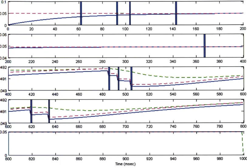
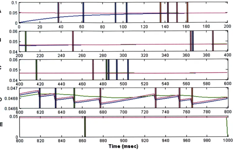
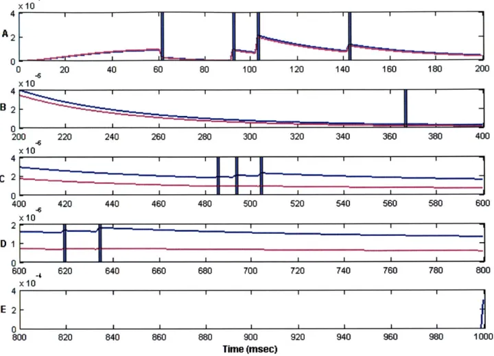
In this chapter we will illustrate how to construct a nonlinear filter for a Point Process model using the Laplace approximation. First we describe the state-space model and its pertinent features and then construct a saddlepoint filter algorithm for estimating the posterior density for this state-space model. We will then present results obtained using our algorithm and compare these results against those obtained using an existing filter.

4.1 Description of the Point Process Model

The Observation Process

Let (0,T] be an observation interval during which the spiking activity of J independent point processes is recorded. For the ith point process the observations consist of the set

of spike times 0< u <ui2 <,---.<UiKi T. For any time t in the observation interval let

N .,(t) be the sample path of the ith point process. It is defined as the event N , = {0 <u <Ui2 <,--..<Uk itflN,(t)=k} where N,(t) is the number of events in (0,t] and k <K,. The sample path is a right continuous function that jumps by 1 at the event times and is constant otherwise [Snyder & Miller, 1991]. This function tracks the location and number of spikes in (0,t] and therefore contains all the information in the sequence of event times. We use No:, = {N ,,N§ } to represent the ensemble activity in (0, t].