Customer focused collaborative demand planning

Customer Focused Collaborative Demand Planning

Ratan Jha

M.S. Industrial Engineering, The University of Arizona, 2004

B.E. Civil Engineering, Maulana Azad National Institute of Technology, 1999

Submitted to the Engineering Systems Division in Partial Fulfillment of the Requirements for the Degree of

Master of Engineering in Logistics

Massachusetts Institute of Technology

© 2008 Ratan Jha All rights reserved

The author hereby grants to MIT permission to reproduce and to distribute publicly paper and electronic copies of this thesis document in whole or in part.

Signature of A uthor ... .. .. ...

Master of Engineering in Logistics Program, Engineering Systems Division May 9, 2008

Certified By...

...

. ...

.

Dr. Lawrence Lapide Director, Demand Management, MIT Center for Transportation & ogistics Thesi pervisor

#U"-Accepted By ... ...

/

Customer Focused Collaborative Demand Planning

by

Submitted to the Engineering Systems Division on May 9, 2008 in Partial Fulfillment of the Requirements for the Degree of Master of Engineering in Logistics

Abstract

Many firms worldwide have adopted the process of Sales & Operations Planning (S&OP) process where internal departments within a firm collaborate with each other to generate a demand forecast. In a collaborative demand planning process buyers and sellers collaborate with each other to generate a mutually agreed upon forecast which takes into account the needs and limitations of both buyers and sellers.

In this research we concentrate on finding out the value from both statistical and qualitative forecasts. We apply standard forecasting algorithms to generate a statistical forecast. We also generate a hybrid model that is a weighted technique using both a statistical and qualitative forecast. Then we evaluate the statistical, hybrid, and qualitative collaborative forecasts using an error analysis methodology. Finally we recommend an approach for forecasting a family of items based on our analysis and results. We also recommend changes to the existing process so that our recommendations on the forecasting approach can get seamlessly integrated into the overall process.

Thesis Supervisor: Dr. Lawrence Lapide

Acknowledgements

There are many people I would like to acknowledge for their assistance and support throughout the pursuit of this research. Unfortunately, many will go unnamed here. For those who are not mentioned, please know that your words of encouragement made a difference.

First of all, I would like to express my sincere gratitude to Dr. Larry Lapide, my advisor, for all of his support and guidance throughout this endeavor. I would also like to thank Dr. Chris Caplice for his accessibility and support regardless of his busy schedule.

I would like to thank my sponsor Jonathan Melzar and all others from his team for help, support and availability, as well as the Demand Management Solutions Group.

I would like to thank my friends at MLOG particularly Prashant Nagpure for always lending a patient ear to my arguments. Finally, I would like to thank my wife Prachi Vimal. Without her

Table of Contents

1. Introduction ... 1

1.1 M otivation... 1

1.2 Supply Chain Excellence... 2

1.3 Collaborative Planning Process... 3

1.4 AS-IS P rocess... 3

2. Methods... ... 5

2.1 Collaborative Planning Forecasting & Replenishment (CPFR)... 5

2.2 Forecasting ... 6

2.2.1 The Simple Moving Average... 7

2.2.2 Simple Exponential Smooting ... 9

2.2.3 Holt's Method for Trend Model ... 9

2.2.4 Damped Method for Trend Model ... ... 10

2.2.5 Croston's Method for Intermittent Demand ... 11

3. Data Analysis ... 13

3.1 Analysis of Product A Family ... 16

3.1.1 Analysis of Product Type - Assembly & Board... ... 16

3.1.1.1 Analysis of PIDs for Product Type -Assembly... 17

3.1.1.2 Analysis of PIDs for Product Type -Board... 19

3.1.2 Analysis of Product Type - Base & Cable ... ... 20

3.1.2.1 Analysis of PIDs for Product Type -Base ... ...22

3.1.2.2 Analysis of PIDs for Product Type -Cable... 23

3.1.3 Analysis of Product Type - Memory & Router... ... 23

3.1.3.1 Analysis of PIDs for Product Type -Memory...25

3.1.3.2 Analysis of PIDs for Product Type -Router... ... 26

3.1.4 Analysis of Product Type - Power ... ... 28

3.2 Analysis of Product B Family ... 30

3.2.1 Analysis of Product Type - Assembly & Board... ... 30

3.2.1.1 Analysis of PIDs for Product Type -Assembly... ...31

3.2.1.2 Analysis of PIDs for Product Type -Board... 32

3.2.2 Analysis of Product Type - Base & Feature... ... 33

3.2.2.1 Analysis of PIDs for Product Type -Base ... ... ... 34

3.2.2.2 Analysis of PIDs for Product Type -Feature... ... 35

3.2.3 Analysis of Product Type - Power & Cable... ... 36

3.2.3.1 Analysis of PIDs for Product Type -Power...37

3.2.3.2 Analysis of PIDs for Product Type -Cable... ... 38

4. Analysis of Statistical Results ... 40

4.1 Forecast Analysis of Product Family A... ... 40

4.1.1 Forecast Analysis of Product Type -Assembly... ... 41

4.1.2 Forecast Analysis of Product Type -Base... ... 42

4.1.3 Forecast Analysis of Product Type -Memory ... 43

4.1.4 Forecast Analysis of Product Type -Router... ... 45

4.1.5 Forecast Analysis of Product Type -Board... ... 46

4.1.6 Forecast Analysis of Product Type -Cable ... 48

4.1.7 Forecast Analysis of Product Type -Power ... ... 49

4.2 Forecast Analysis of Product Family B... ... 50

4.2.1 Forecast Analysis of Product Type -Assembly... ... 50

4.2.2 Forecast Analysis of Product Type -Base ... .... ... 52

4.2.3 Forecast Analysis of Product Type -Switch... ... 53

4.2.4 Forecast Analysis of Product Type -Feature... ... 54

4.2.5 Forecast Analysis of Product Type -Board ... .... . 56

4.2.6 Forecast Analysis of Product Type -Cable ... ... 57

4.2.7 Forecast Analysis of Product Type -Power ... ... 58

4.3 Sum m ary of Results... ... 60

5. Comparison Between Statistical and Qualitative Forecast ... 64

5.1 Analysis of Product Family A ... 64

5.2 Analysis of Product FamilyB ... 66

6. Recommendations & Future Research ... ... 69

List of Tables

Table 1: Parameter List for Assembly & Board ... 17

Table 2: Parameter List for Base & Cable... 22

Table 3: Parameter List for Memory & Router ... 25

Table 4: Parameter List for Assembly & Board ... 31

Table 5: Parameter List for Base & Feature ... 34

Table 6: Parameter List for Power & Cable ... 37

Table 7: MAD of different forecasts for Assembly ... 41

Table 8: RMSE of different forecasts for Assembly...41

Table 9: MAD of different forecasts for Base ... 42

Table 10: RMSE of different forecasts for Base ... 43

Table 11: MAD of different forecasts for Memory ... 44

Table 12: RMSE of different forecasts for Memory ... ... 44

Table 13: MAD of different forecasts for Router ... 45

Table 14: RMSE of different forecasts for Router... 46

Table 15: MAD of different forecasts for Board ... 47

Table 16: RMSE of different forecasts for Board ... 47

Table 17: MAD of different forecasts for Cable ... 48

Table 18: MAD of different forecasts for Cable ... 48

Table 19: MAD of different forecasts for Power ... 49

Table 20: RMSE of different forecasts for Power ... 50

Table 21: MAD of different forecasts for Assembly ... 51

Table 22: RMSE of different forecasts for Assembly ... 51

Table 23: MAD of different forecasts for Base... 52

Table 24: RMSE of different forecasts for Base... 52

Table 25: MAD of different forecasts for Switch ... 53

Table 26: RMSE of different forecasts for Switch ...54

Table 27: MAD of different forecasts for Feature...55

Table 28: RMSE of different forecasts for Feature...55

Table 29: MAD of different forecasts for Board ... 56

Table 30: RMSE of different forecasts for Board ... 56

Table 31: MAD of different forecasts for Cable ... 57

Table 32: MAD of different forecasts for Cable ... 58

Table 33: MAD of different forecasts for Power ... 59

Table 34: RMSE of different forecasts for Power ... 59

Table 35: RMSE of Type, BUF and Hybrid for family A Types ... ... 60

Table 36: RMSE of Type, BUF and Hybrid for family B Types ... ... 62

Table 37: RMSE of QF, BUF and HF for family A PIDs ... 65

List of Figures

Figure 1: VICS CPFR Model ... 6

Figure 2: Family A Hierarchy ... 13

Figure 3: PID Distribution for Product Family A ... 13

Figure 4: Family B Hierarchy ... 14

Figure 5: PID Distribution for Product Family B ... 14

Figure 6: Weekly Demand Pattern for Assembly & Board ... 16

Figure 7: Forecast vs Actuals for Assembly & Board ... 17

Figure 8: Weekly demand pattern for PIDs of Assembly with continuous demand ... 18

Figure 9: Weekly demand pattern for selected PIDs of Assembly with Intermittent dem and ... 18

Figure 10: Weekly demand pattern for PIDs of Board with continuous demand...19

Figure 11: Weekly demand pattern for selected PIDs of Board with Intermittent dem and... ... 20

Figure 12: Weekly Demand Pattern for Assembly & Board ... ... 21

Figure 13: Forecast vs Actuals for Base & Cable ... 21

Figure 14: Weekly demand pattern for selected PIDs of Base with Intermittent dem and... ... 22

Figure 15: Weekly demand pattern for selected PIDs of Cable with Intermittent dem and... ... 23

Figure 16: Weekly Demand Pattern for Memory & Router ... 24

Figure 17: Forecast vs Actuals for Memory & Router ... ... .... 24

Figure 18: Weekly demand pattern for PIDs of Memory with continuous demand...25

Figure 19: Weekly demand pattern for selected PIDs of Memory with Intermittent dem and... ... 26

Figure 20: Weekly demand pattern for PIDs of Router with continuous demand...27

Figure 21: Weekly demand pattern for selected PIDs of Router with Intermittent dem and... ... 27

Figure 22: Weekly Demand Pattern for Power...28

Figure 23: Forecast vs Actuals for Power...29

Figure 24: Weekly demand pattern for selected PIDs of Powew with Intermittent dem and... ... 29

Figure 25: Weekly Demand Pattern for Assembly & Board ... 30

Figure 26: Forecast vs Actuals for Assembly & Board...31

Figure 27: Weekly Demand Pattern for Selected PIDs of Assembly...32

Figure 28: Weekly Demand Pattern for Selected PIDs of Board...32

Figure 29: Weekly Demand Pattern for Base & Feature ... ... 33

Figure 30: Forecast vs Actuals for Base & Feature ... 34

Figure 31: Weekly Demand Pattern for Selected PIDs of Base ... 35

Figure 32: Weekly Demand Pattern for Selected PIDs of Feature ... 35

Figure 33: Weekly Demand Pattern for Power & Cable ... ... .... ... ...36

Figure 34: Forecast vs Actuals for Power & Cable ... ... 36

Figure 35: Weekly Demand Pattern for Selected PIDs of Power...37

Figure 37: Weekly Demand Pattern for Switch ... 39

Figure 38: Type, BUF and Hybrid RMSE for Family A... ...61

Figure 39: Type, BUF and Hybrid RMSE for Family B... ...62

Figure 40: QF, BUF and HF RMSE for family A ... 66

Figure 41: QF, BUF and HF RMSE for family B ... 68

Figure 42: System A -Statistical Forecasting...71

Figure 43: System B -Composite Forecasting... 72

Chapter 1: Introduction

This section describes the motivation of this research. The section goes on to explain the current process at HiTec Inc and a brief background of HiTec Inc and Wireless Inc.

1.1 Motivation

Collaborative planning has increasingly gained significance over the years with the strengthening of information infrastructures. Buyers and Suppliers can share their information such as capacity and demand so that they can plan their resources in a better way.

One important aspect of collaborative planning is Collaborative Planning Forecasting and Replenishment (CPFR). CPFR facilitates communication between a buyer and a supplier about the expected future demand and supply availability. Once the supplier has visibility of the future demand from the buyer, the supplier can plan better on raw materials procurement and save on costs related to uncertainty. CPFR model works even better when the customer is a large account and constant business transaction takes place between the buyer and the supplier. Collaboration helps the supplier to serve the customer better by knowing the future needs of the buyer. Collaborative planning tries to solve the problem of stock outs of critical products and of excessive safety stock that shows on the balance sheet.

The scope of my thesis is to determine how the benefits of collaborative planning can be leveraged to reduce the lead time variability and to increase the probability of a product's availability when it is demanded.

The thesis looks at the current collaborative planning process between HiTec Inc and Wireless Inc, who is a strategically important customer of HiTec Inc. Wireless Inc is one of the biggest

customer of HiTec Inc and HiTec Inc wants to explore whether there is any opportunity of improvement in the current collaborative planning and forecasting process. HiTec Inc wants to use the recommendations of this research to leverage their current service to the Wireless Inc and enhance the strategic alliance thus creating opportunities for further revenue and profits. It also wants to consider extending the recommendations of this research to other important customers.

1.2 Supply Chain Excellence

HiTec Inc today is a leader in supply chain management and logistics. HiTec Inc is the best examples of the virtual supply chain organization where all the logistic activities have been

outsourced to 3PLs. There are various risks and benefits associated with being a virtual supply chain organization. HiTec Inc has been successful over the years because it was able to create a business model where the benefits of virtual supply chain outweighed the risks. One of the primary drivers of this model has been their focus on supply chain excellence (SCMx). SCMx is a state where the entire supply chain organization within HiTec Inc would deliver excellence in wherever they can establish their position as market leaders and innovators. HiTec Inc has identified some initiatives that would help them to get to a state of SCMx. Each business unit within the manufacturing organization in HiTec Inc has been following these initiatives and identifying new ones to achieve the desired goal. The scope of this thesis is limited towards studying a few of those initiatives followed by the collaborative planning business sub-unit within the demand planning business unit that sits under the supply chain organization of HiTec Inc.

1.3 Collaborative Planning Process

The intent of following a collaborative planning process was to provide excellent customer service in terms of timely order fulfillment to a select group of strategic clients. This process would protect the customer from supply variability due to unpredictable demand from other customers. The process would also ensure predictable and consistent delivery performance. The customer would be directly linked with HiTec Inc's supply chain which would help in quick response to the demand signal.

HiTec Inc would benefit from this process because a customer would be able to derive satisfaction due to improved delivery performance that would help in building strategic relationships. From the organizational point of view the collaborative planning process would help in the integration of sales & marketing, manufacturing and fulfillment, and enable them to

work together to manage high revenue drivers.

1.4 AS-IS Process

As part of the current collaborative planning process, the team from the collaborative planning sub-unit interacts with the customer to generate a 120-day rolling forecasts for products each month. The 120-day rolling forecast is then broken into four months denoted by M+1, M+2, M+3, M+4 where M is the current month in which a forecast is generated. As the customer makes actual bookings, the booking numbers are deducted from the forecast numbers. At the end of the month if bookings are less than the forecasts, the quantity not used in the month does not

get covered in the subsequent months but an updated forecast is generated each month to reflect the month to month changes.

Based on the 120-day rolling forecast, HiTec Inc makes a commitment for the availability of raw materials for the manufacturing of products. The supply reservations (SR) are calculated based

on the standard product target and lead time. The SR for the current month expires if there are not sufficient days left to meet the target lead time. The expired SR does not get automatically rolled in the next month but has to be reflected as a change in forecast and a new SR has to be

generated. SR information is updated weekly based on the information on available supply. The 120-day rolling forecast does not guarantee supply availability. Based on the forecast and supply of raw materials, demand is matched with supply and SR commitments are provided to the customer. Currently the demand and supply is matched manually and an automated process is not being used.

The marketing department also generates a quarterly forecast based on the bookings to generate expected revenues. The expected revenue is used as the basis for ordering raw materials for manufacturing.

One important role of the collaborative planning team is to make sure that the marketing forecast and the 120-day rolling forecast are aligned so that there is no mismatch between the

manufacturing component orders and the customer forecast.

The success of the current process is measured by metrics such as forecast accuracy, delivery performance to target lead time and delivery performance to promise.

Chapter 2: Methods

To validate the collaborative planning process it is necessary to compare it with Collaborative Planning, Forecasting and Replenishment (CPFR) Model. We can apply the CPFR model in the current scenario to better understand the collaborative process.

It is also necessary to conduct research on the forecasting algorithms such as Moving Averages, Single Exponential Smoothing and Holt' s Smoothing because these methods would be later used to analyze the current forecasting process and would also be used to generate a statistical forecast on a weekly basis.

2.1 Collaborative Planning Forecasting and Replenishment (CPFR)

CPFR is collaborative planning process which was conceptualized by the Voluntary Inter-industry Commerce Standards Association (VICS). VICS is an association of companies that defines processes which would help an organization in achieving seamless flow of products and information across their supply chain. CPFR is constituted by a VICS committee whose mission is to develop best practices for various collaborative planning scenarios. The processes include suppliers and retailers and helps in evolving an integrated planning approach.

Figure 1 below shows the VICS Framework CPFR. In the framework the consumer is placed at the center and is represented by a circle. The Retailer is represented by a concentric circle with a larger diameter compared to the consumer. The Retailer circle lists the activities to be performed by the retailer starting with Point of Sales (POS) forecasting with subsequent activities moving in clockwise direction. The concentric circle, outside the retailer circle, with arrows, depicts the

collaborative activities that need to be undertaken. Finally the activities outside the biggest circle represent an aggregated planning approach recommended by the CPFR committee.

Figure 1: VICS CPFR Model (Source: VICS CPFR Committee)

Although the CPFR model was built keeping retail supply chains in mind, it can be extended to other supply chains as well where collaborative planning is integral part of the chain.

2.2 Forecasting

Forecasting is the stepping stone for Supply Chain Planning and Management. All the upstream planning decisions such as inventory planning, logistics planning and production planning depend on the forecast numbers. An accurate forecast is the key to reduce costs and achieve

reductions in inventory levels. Although it's impossible to achieve 100% forecast accuracy, accuracy levels in the range of 90-100% are desirable. The forecast accuracy depends on the variability of the demand which essentially means that we can have more accurate forecasts for demand with less variability. Forecasts are much more accurate at the aggregate level. As the granularity, of the level at which we are generating a forecast, increases the accuracy decreases. Forecasts can be generated for both operational and strategic requirements. Operational forecasts are used in short term planning and execution and more often than not statistical time-series methods are used to produce operational forecasts. Operational forecasts are generated on a daily, weekly or monthly basis. Long term forecasts are produced for strategic reasons. For example if we want to know the impact of macroeconomic factors on our sales we look at the long term forecast which has a window of more than a year. Causal techniques are used to generate long term forecasts.

The scope of this work includes forecast generation on a monthly and weekly basis so we will only discuss operational forecasting. Besides aggregation, selection of an appropriate statistical model is also important for achieving better forecast accuracy. We have discussed a few Time-Series models that have widespread use in operational forecasting. The models evaluated or used for the purpose of the thesis are discussed in the subsequent sections. All the equations and expressions are adapted from Silver, Pyke and Peterson (1998).

2.2.1 The Simple Moving Average

The simple moving average is a smoothing procedure where an average of N periods is

periods. In the next N periods the first period in the current period is removed and the (N+1)t

period relative to the current period is included. The demand can be modeled as in equation 2.1:

x, =a+Cet --- (2.1)

x, = actual demand in period t.

a = level estimate

e, = random noise

The equation shows that the demand in period t can be represented as a level component which is a constant and a random noise (e,).

The N-period moving average (xt.N) is given by the equation:

Xt,N = (Xt + Xt_1 + Xt-2 t... + ,N+ ) / N --- (2.2)

In equation 2.2, xt represents the actual demand. The level estimate in period t can be given by

i_t = Xt,N --- (2.3)

We can forecast the demand for period t+k at the end of period t using the equation:

2.2.2 Simple Exponential Smoothing

A moving average procedure gives equal weights to each period for calculating the forecast. This

procedure has limitations because the underlying demand model may be such that different weights might be required for each period. Simple exponential smoothing does exactly that, as follows:

The underlying demand model: x, = a + e, --- (2.5)

Level Estimate: a, =

ax

a is a smoothing constant and it can be approximated as a = 2/(N+l) --- (2.7)

The initial estimate of a is found by considering the average of the first few periods of demand and the forecast model is the same as in equation 2.4

2.2.3 Holt's Method for Trend

In the previous discussions we assumed that a demand forecast has only a level component and does not have any trend. If our data is showing an increasing trend with time then we should apply a smoothing procedure that takes care of the trend in the underlying demand model, as follows:

The underlying demand model: x, = a + bt + e, --- (2.8)

The variable b represents the trend with respect to the time t.

a, = a, +(1- a)(t,_1 + b,_) --- (2.9)

b, = (, - _) + (1- )b,_ --- (2.10)

a and flare smoothing constants.

The initialization for level and trend components can be done using regression techniques and the forecasts are generated using the following equation.

t,t+k =t +bk --- (2.11)

;t,t+k = forecast of the demand in time period t+k at the end of time period t.

i,

b, = estimate of trend at the end of time period t.

2.2.4 Damped Method for Trend Model

When the data has lot of random noise, it is very difficult to spot a trend. If the forecasting requirement is to project trend several periods ahead then the simple trend model does not give a clear picture because the trend may not be linear. The damped trend model is very useful for forecasting when history has a lot of noise and trend is not clear. This model is very similar to the Holt's model. An additional dampening parameter is introduced in the Holt's model to give us damped trend model, as follows:

b

(2.13)

where 0 is a dampening parameter. When = 1 then the above equations transforms to Holt's model.

Following is the forecasting model.

k

at,t+k =a + ---_ (2.14)

i=1

If 0 < 0 < 1 then the trend is damped and as k gets large, the forecast tends to a horizontal line. When 0 > 1, the trend becomes exponential.

2.2.5 Croston's Method for Intermittent Demand

Croston's method is used to generate forecasts for intermittent or erratic demand. When demand occurrences are infrequent then the exponential smoothing process does not produce the desired level forecast. In such cases the demand is modeled as two separate components.

The inter arrival time between non zero demand is the first component that is modeled as a random variable obeying a normal distribution. In any given period, the demand xt can be modeled as,

Xt =Yt*Zt --- (2.15)

where, yt = 1 if demand occurs otherwise y, = 0 and zt is the magnitude of the demand.

As mentioned above, the inter arrival time between demand can be modeled as a random variable. Let n be the time between consecutive non zero demands. Either a demand in a given

period will occur or it will not occur. Thus, the event can be modeled as a Bernoulli's process with the probability of occurrence of non zero demand as 1/n.

prob (yr = 1) = 1/n and prob (y, = 0) = (1 - 1/n)

Croston (1972) proposed a framework for an updating procedure based on assumptions stated above.

If the demand is zero in a particular period then, a) Demand estimates are not updated and

b)

n,

=

,_,

---

(2.16)

If the demand is non-zero in a particular period then,

a) = at + (1- a) --- ----- (2.17)

b) n, = ant +(1-a),_ ---- - - (2.18)

Where,

n,= number of periods since the last event of occurrence of non-zero demand.

,t

2, = estimate of the average size of demand at the end of period t.

Chapter

3:

Data Analysis

We were provided with data of two product families, A & B. Each product family can be subdivided into product types and each product type can be further subdivided into Product Identities (PIDs). PIDs are at the lowest level in the product hierarchy. The requirement here is to analyze product level data for a fixed geography which is the world level. The time hierarchy is characterized by year, month and weeks. The data is provided in weekly buckets which can be aggregated into monthly and yearly buckets. Figure 2 shows the hierarchy for family A. Each product type can be further subdivided into PIDs. Product A has a total of 133 PIDs. Figure 3 shows the distribution of PIDs among each product type.

Figure 2: Family A Hierarchy

Family A

Figure 3: PID Distribution for Product Family A

Figure 4 shows the hierarchy for family B. Each product type can be further subdivided into PIDs. Product B has a total of 137 PIDs. Figure 5 _{shows the distribution of PIDs among each}

product type.

Figure 4: Family B Hierarchy

Family B

30

ojL/

Iq

Cie:

Figure 5: PID Distribution for Product Family B

The following subsections of this chapter present the data pattern of each product type under families A & B. Also, data patterns of some selected PIDs under each product type for family A

14

I _{I _I I _· I _ _}

& B are also presented. Graphs, charting generated statistical forecast and history for the 19 week time period are also presented.

A Damped trend model was used to generate a forecast at product type level. If the product type has intermittent demand pattern then 20-period moving average technique was applied. Any product type or PID which had occurrence of events having zero demand for three consecutive period more than twice was deemed as type or PID having an intermittent demand pattern.

Croston's method was not applied for intermittent demand pattern because the method assumes a normal distribution for non-zero demand occurrences. For almost all the types or PIDs this assumption was not satisfied because of the limited availability of data and a large number of occurrences of non-zero demand; thus Croston's method was found unsuitable for our purpose. Smoothing parameters, Holt's alpha and beta and dampening constants for the damped trend model and Root Mean Square Error (RMSE) of each forecast is also tabulated in sections below. Brown (1963) showed that for given values of parameter a the Holt's alpha and beta parameter can be estimated using the following formula.

allw = [1- (1- a)2] ... (3.1) a,

3.1

_{Analysis of Product A family}

This section presents the analysis of data for different product types and their associated PIDs.

3.1.1 Analysis of Product Type - Assembly & Board

Weekly Demand Pattern

4UU 0 350 U 300 n 250 i 200 t 150 s 100 50

7L1L

7117A±-.

Figure 6: Weekly Demand Pattern for Assembly & Board

Figure 6 shows the demand pattern for the Assembly and Board product types. The pattern has a lot of noise and visual analysis does not reveal a trend. Seasonality is also ruled out because the product characteristics are not seasonal. The damped trend model is applicable to this type of pattern because the trend does not follow a fixed pattern.

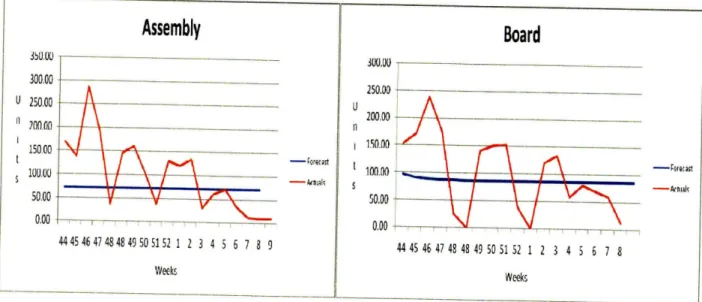
Figure 7 below shows the plot of forecast against the history for Assembly and Board. The application of Holt's method would have produced a negative forecast thus the damped trend model had a better applicability for both Assembly and Board.

Table 1 shows the parameter values, Coefficient of Variation (COV) of the forecast and the root mean square error for Assembly & Board.

U t-i-T-T-T TT-F-r-r-r-rT _{TrT1T-TF-,--tr-}

r-202L262830313335373941434445484951 1 3 5 7 9

Assembly

Figure 7: Forecast vs Actuals for Assembly & Board

alpha (a Hw) beta (flHW) phi (0) RMSE COV

Assembly _{0.51 0.177 0.3}

78.971 111.35%

Board _{0.75 0.33 0.5}

68.129 79.13%

Table 1: Parameter List for Assembly & Board 3.1.1.1 Analysis of PIDs for Product Type - Assembly

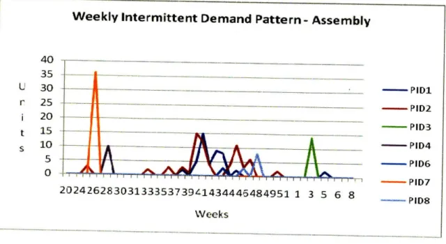
Out of 29 PIDs under Product Type Assembly, six exhibited continuous demand while the rest exhibited intermittent demand. The Damped trend model was applied to those PIDs that exhibited continuous demand while 20-period moving average was applied to PIDs that

exhibited intermittent demand. Figure 8 below shows the weekly demand pattern for continuous PIDs.

--

---

-I

_-~

Board

_A

-Forecast

Weekly Continuous Demand Pattern - Assembly

2D24262830313335373941434446484951 _{1 3 5 7}

Weeks

Figure 8: Weekly demand pattern for PIDs of Assembly with continuous demand Figure 9 shows the weekly demand pattern for some of the PIDs with intermittent demand.

Weekly Intermittent Demand Pattern - Assembly

35 -U 30 r 25-i 20 -t 15 10 --- PID1 .PID2 -- PID3

----

APID4

A&

vY1.

xAe\

6 L%,

2 2 3 3 7 4 8 6 -8pIn/

2024262830313335373941434446484951

1 3 5 6 8 _PID Weeks

Figure 9: Weekly demand pattern for selected PIDs of Assembly with intermittent demand

18 u 45 -40 U 35 n 30 i 25 t 20 15 10 5 - >ID1 -- _IlD2 'ID4 -:'IDS _· __ · VY b

A-

AtAI1

1D

12

101

14v

3.1.1.2 Analysis of PIDs for Product Type - Board

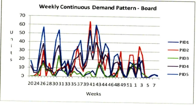
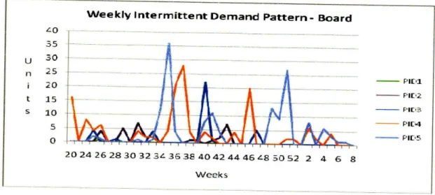
Out of 62 PIDs under product type Board, five exhibited continuous demand while the rest exhibited intermittent demand. Damped trend model was applied to those PIDs that exhibited continuous demand while 20-period moving average was applied to PIDs that exhibited intermittent demand. Figure 10 below shows the weekly demand pattern for continuous PIDs, and Figure 11 shows the weekly demand pattern for some of the PIDs with intermittent demand.

Weekly Continuous Demand Pattern - Board

--- T-

fA-- PID1

--- PID2

- PID3

- PID4

PJf9R$~E% r

9AI-

WItn

VI

2024262830313335373941434446484951 1 3 5 7

Weeks

Figure 10: Weekly demand pattern for PIDs of Board with continuous demand

/u

60

-

a

Weekly Intermittent Demand Pattern - Board

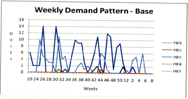
Figure 11: Weekly Demand Pattern for selected PIDs of Board with Intermittent Demand 3.1.2 Analysis of Product Type - Base & Cable

Figure 12 below shows the demand pattern for the Base and Cable product types. As in the case of Assembly and Board the demand pattern of Base and Cable is suitable for applicability of a damped trend model. Figure 13 below shows the plot of forecast against the history for Base and Cable. The application of Holt' s method would have produced a negative forecast as it did in the case of assembly thus damped trend model was applied to the demand pattern of Base and Cable.

35 U 30 n 25 i 20 t 15 s 10 5 0 ---- PlIDa P1(2I~i --- P1i3 - P1(4 --- P115 20 24 26 2830 32 34 _{3638404244 46 8 50052 2 4 6 8} Weeks ,,

Weekly Demand Pattern

-- ~able.

2024262830313335373941434446484951 _{1 3 5 7} Weeks

Figure 12: Weekly Demand Pattern for Base & Cable

Base

Cable

0.00

Figure 13: Forecast vs Actuals for Base & Cable

- Forecast

- Actuas

I - - - --

I---[ore•ast

Table 2: Parameter List for Base & Cable

Table 2 shows the parameter values, COV of the forecast and the root mean square error.

3.1.2.1 Analysis of PIDs for Product Type - Base

Product type Base has 9 PIDs and all these PIDs exhibited intermittent demand. A 20-period moving average technique was applied to all the PIDs.

Figure 14 shows the weekly demand pattern for some of the PIDs belonging to Base.

Weekly Demand Pattern - Base

- - PID1 - PID2 -PID3 _- P1D5 20242628303234363840424446485052 2 468 Weeks

Figure 14: Weekly Demand Pattern for selected PIDs of Base with Intermittent Demand

alpha (a HW) beta (f HW) _phi (0) RMSE COV

Base 0.51 0.177 0.3 11.077 78.55% Cable 0.51 0.17 0.3 11.574 134.88% --- _{I-- I I} -I

I

At I I I I

X I I

VIA I

A

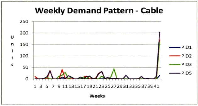
3.1.2.2 Analysis of PIDs for Product Type - Cable

Product type Cable has 6 Pills and all these Pills exhibited intermittent demand. A 20-period moving average technique was applied to all the Pills.

Figure 15 shows the weekly demand pattern for some of the Pills belonging to Cable.

Weekly Demand Pattern - Cable

200 -:>101 -:>102 -:>103 -:>105

o

Figure 15: Weekly Demand Pattern for selected PIDs of Cable with Intermittent Demand

3.1.3 Analysis of Product Type - Memory &Router

Figure 16 below shows the demand pattern for the Memory and Router product types. As in the case of Assembly and Board the demand pattern of Memory and Router is suitable for

applicability of a damped trend model. Figure 10 below shows the plot of forecast against the history for Memory and Router.

Weekly Demand Pattern

1

i

Figure 16: Weekly Demand Pattern for Memory & Router

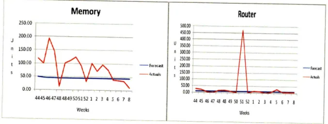
Table 3 shows the parameter values, COV of the forecast and the root mean square error.

Memory

Router

Figure 17: Forecast vs Actuals for Memory & Router

Memory -Router -Forecast -Actuals

A

A

f I I kil

I i R IV

ITION-JV

_{V V I/}

-Table 3: Parameter List for Memory & Router

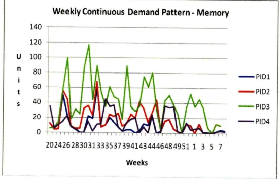
3.1.3.1 Analysis of PIDs for Product Type - Memory

Out of 22 PIDs under product type Memory, four exhibited continuous demand while the rest

exhibited intermittent demand. A Damped trend model was applied to those PIDs that exhibited continuous demand while 20-period moving average was applied to PIDs that exhibited

intermittent demand. Figure 18 below shows the weekly demand pattern for continuous PIDs.

140 120 100 80 60 40 20 0

Weekly Continuous Demand Pattern - Memory

I 2024262830313335373941434446484951 1 3 5 7 Weeks -PID1 - PID2 - PID3 -- PID4

Figure 18: Weekly Demand Pattern for PIDs of Memory with Continuous Demand

alpha (a H.) beta ( HW) phi (0) RMSE COV

Memory 0.75 0.33 0.5 60.835 136.51%

Router 0.51 0.17 0.8 8.559 82.57%

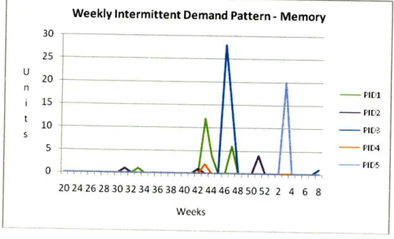
-I--Figure 19 shows the weekly demand pattern of some of the PIDs with intermittent demand

Weekly Intermittent _{Demand Pattern - Memory}

SU 25 20 n i 15 t ₁₀ S 5 0 - PID1 - PID2 - PID3 --- PID5_{P11)5- IU}

Figure 19: Weekly Demand Pattern for selected PIDs of Memory with Intermittent Demand

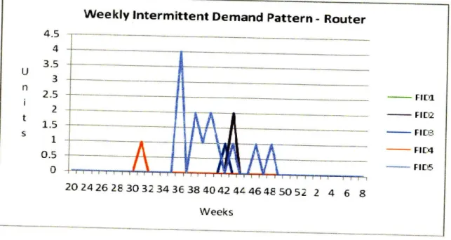
3.1.3.2 Analysis of PIDs for Product Type - Router

Out of 14 PIDs under product type Router, only one exhibited continuous demand while the rest exhibited intermittent demand. Damped trend model was applied to the PID that exhibited continuous demand while 20-period moving average was applied to PIDs that exhibited intermittent demand. Figure 20 below shows the weekly demand pattern for continuous PID

~

~-~---20242628303234363840424446485052 2 4 6 8

Weekly Continuous Demand Pattern - Router

2024262830313335373941434446484951 1 3 5 7

20242262830313335 373941434446484951 1 3 5 7

- PID1

Weeks

Figure 20: Weekly Demand Pattern of PIDs with Continuous Demand

Figure 21 shows weekly demand pattern for some of the PIDs exhibiting intermittent demand.

Weekly Intermittent _{Demand Pattern - Router}

4.5 4 3.5 3 2.5 2 1.5 1 0.5 0

N A

~r

Figure 21: Weekly Demand Pattern for selected PIDs of Router with Intermittent _Demand

I

1-

11 M A-A

11~

)

1

---

3.1.4 Analysis of Product Type - Power

Figure 22 shows the weekly demand pattern for product type Power. It can be seen that this product type exhibits intermittent demand. Croston's method is a suitable model to apply to this kind of demand pattern but as discussed at the start of the section a 20-period moving average was applied to the Power type.

Weekly

Demand Pattern

45 40 -U 35 -n 30-i 25 t 20 -15 10

5o

Figure 22: Weekly Demand Pattern for Power

Figure 23 shows the plot of forecast against history for Power. The important point here is the forecast would be level because we are using a moving average smoothing technique.

Power

Figure 23: _{Forecast vs Actuals}

3.1.3.1 Analysis of PIDs for Product Type - Power

Product type power has 9 PIDs and all these PIDs exhibited intermittent demand. A 20-period moving average technique was applied to all the PIDs. Figure 24 shows the weekly demand pattern for some of the PIDs belonging to power product type.

RMSE for power was 2.94 and COV was 294%.

Weekly Demand Pattern - Power

PIDI -- PID2 PID3 -- PID4 -- PID5

Figure 24: Weekly Demand Pattern of selected PIDs with Intermittent Demand

20 24 26 28 30 32 34 36 38 40 42 44 46 48 50 52 2 4 6 8 Weeks _ __ __I

I

3.2

_{Analysis of Product B family}

This section presents the analysis of data for different product types and their associated PIDs.

3.2.1 Analysis of Product Type - _{Assembly & Board}

Weekly Demand Pattern

1400 -1200 U 1000 n 800 0n0 ---t 400 200 0 -Assembly - Board

Figure 25: Weekly Demand Pattern for Assembly & Board

Figure 25 _{shows the demand pattern for the Assembly and Board product types. The pattern has}

a lot of noise and visual analysis does not reveal a trend. Seasonality is also ruled out because the product characteristics are not seasonal. Product type assembly exhibited characteristics that make the application of a moving average model suitable. Assembly type had two occurrences of patterns where three or more periods of zero demand was observed. Product type Board

exhibited no such characteristic so a damped trend model was applied.

Figure 26 below shows the plot of forecast against the history for Assembly and Board. A 20-period moving average technique was applied to product type, assembly.

Table 4 shows the parameter values, COV of forecast and the root mean square error.

2024262830313335373941434446484951 1 3 5

Assembly

30

---15000

Figure 26: Forecast vs Actuals for Assembly and Board

alpha (a HW) beta (/3 Hw) phi (0) _{RMSE COV}

Assembly _{0.51 0.18 0.3 72.85}

107.05%

Board _{0.51 0.18 0.4}

250.9 2280.97%

Table 4: Parameter List for Assembly & Board 3.2.1.1 Analysis of PIDs for Product Type - Assembly

Product type Assembly has 16 PIDs and all these PIDs exhibited intermittent demand. A 20-period moving average technique was applied to all the PIDs. Figure 14 shows the weekly demand pattern for some of the PIDs belonging to Board.

Board

Assembly

Figure 27: Weekly demand pattern for selected PIDs of Assembly 3.2.1.2 Analysis of PIDs for Product Type - Board

Product type Board has 62 PIDs and all these PIDs exhibited intermittent demand. A 20-period moving average technique was applied to all the PIDs. Figure 14 shows the weekly demand pattern for some of the PIDs belonging to Board.

Board

Figure 28: Weekly demand pattern for selected PIDs of Board

I.U

7

22 24 26 28 30 32 34 36 38 40 42 44 46 48 50 52 2 4 7

Weeks

3.2.2 Analysis of Product Type - Base & Feature

Figure 29 shows the demand pattern for the Base and Feature product types. The pattern has a lot of noise and visual analysis does not reveal a trend. Seasonality is also ruled out because the product characteristics are not seasonal. Product type Base exhibited characteristics that make the application of moving average model. Base type had two occurrences of pattern where three or more periods of zero demand was observed. Product type Feature exhibited no such

characteristic so a damped trend model was applied.

Weekly Demand Pattern

450U 400 350 300 250 200 t 150 s 100 50 0 - Base - Feature 2024262830313335373941434446484951 _{1 3 5 7} Weeks

Figure 29: Weekly Demand Pattern for Base & Feature

Figure 30 below shows the plot of forecast against the history for Base and Feature. A 20-period moving average technique was applied to product type Base and a damped trend model was applied to product type Feature.

Base

Feature

Figure 30: Forecast vs Actuals for Base & Feature

alpha (a HW) beta ( fHW) phi (0) RMSE COV

Base 0.51 0.18 0.3 22.676 97.32%

Feature 0.0975 0.023 0.8 91.227 113.83%

Table 5: Parameter List for Base & Feature

Table 5 shows the parameter values, COV of forecast and the root mean square error.

3.2.2.1 Analysis of PIDs for Product Type - Base

Product type Base has 9 PIDs and all these PIDs exhibited intermittent demand. A 20-period moving average technique was applied to all the PIDs.

Figure 31 shows the weekly demand pattern for some of the PIDs belonging to Base.

44 45 46 47 48 48 49 50 51 52 1 2 3 4 Weeks - Forecast -Actuals 5 6 7 8 I _ __I

Weekly Demand Pattern

- Base

Figure 31: Weekly Demand Pattern for selected PID of Base 3.2.2.2 Analysis of PIDs for Product Type - Feature

Product type feature has 20 PIDs and all these PIDs exhibited intermittent demand. A 20-period moving average technique was applied to all the PIDs.

Figure 32 shows the weekly demand pattern for some of the PIDs belonging to Feature.

Weekly Demand Pattern- Feature

~--a_~

_-_ALJIA

_IL

_A~~

Figure 32: Weekly Demand Pattern for selected PIDs of Feature

.I~

-'-~'-~~I- ~~~~-` `~-~-~---~-~` ' --- I~-- ~~-~~I-~~--~x ~~ ~~-I~x~~~-~~-~^`~----~--~-- _{--- ~~ ~~-~~~~-~~-~`~^--}

~----~~~--~-~-"

~-~---~-~-~~~-'''''i';l''l'''"'

3.2.3 Analysis of Product Type - Power & Cable

Figure 33 shows the demand pattern for the Cable and Power product type. Product type Power exhibited characteristics that make the application of moving average model. Power type had two occurrences of pattern where three or more periods of zero demand was observed. Product type Cable exhibited no such characteristic so a damped trend model was applied.

Weekly Demand Pattern

I-

-

-2024262830323L363840424446485052 _{2 4 6 8}

Weeks

Figure 33: Weekly Demand Pattern for Power & Cable

Figure 34 shows the plot of the forecasts against the actuals.

Power - Forecast - Actuals --- --- --- --- ---444546474849505152 _{1 2 3 4 5 6 7 8} Weeks Cable 45.00 40.00 35.00 30,00 25.00 20.00 15.00 10.00 0.00 i--- ----;-- -- - - - -444546 47484849505152 _{1 2 3 4 5 6 7 8} Weeks

Figure 34: Forecast vs Actuals for Power and Cable

Power Cable 25 U 20 n I 15 10 - Forecast -Actuals

_

~

_{__}

II---~---Table 6: Parameter List for Power & Cable

Table 6 shows the parameter values, COV of the forecast and the root mean square error. 3.2.3.1 Analysis of PIDs for Product Type - Power

Product type Power has 16 PIDs and all these PIDs exhibited intermittent demand. A 20-period moving average technique was applied to all the PIDs.

Figure 35 below shows the weekly demand pattern for some of the PIDs.

Weekly

_{Demand Pattern- Power}

-i---·zkiz---1A

!

k-

A ...

M1 ....

t-i

\

I , A

Figure 35: Weekly Demand Pattern for Selected PIDs of Power

alpha (a Hw) beta ( HW) _{phi (0) RMSE COV}

Power _{0 0}

0 8.85 102.89%

Cable _{0.5 0.18}

0.3 9.216 118.36%

--- ~--~- -~- _I-`

3.2.3.2 Analysis of PIDs for Product Type - Cable

Product type Cable has 11 PIDs and all these PIDs exhibited intermittent demand. A 20-period moving average technique was applied to all the PIDs.

Figure 36 shows weekly demand pattern for some of the PIDs exhibiting intermittent demand.

Weekly Demand Pattern

_-

Cable

45 40 U t---·---

-V

Figure 36: Weekly Demand Pattern of selected PIDs of Cable 3.2.3 Analysis of Product Type - Switch

Figure 38 shows the demand pattern for the Switch product type. Product type Switch exhibited characteristics that make the application of moving average model. Switch type had two

occurrences of pattern where three or more periods of zero demand was observed.

--Weekly Demand Pattern

II

A

AJ1/1

A

_I-l/In

11

_

ILI

•-

Figure 37: Weekly Demand Pattern for Switch

RMSE for switch was 2.055 _{and the COV was 93.39%.}

_ _ _~ _ _{_ _ __ _} ___ I_ _I_ 20 _ ____ 242 83 3 ____ 33 _ 7 94 ___ 3444 84 5

f NJ

----

---

-

I~lcJv vV

Chapter 4: Analysis of Statistical Results

This section compares the forecast generated at the product family level with the forecast generated at the PID level and aggregated up to the product type level, called the Bottom up Forecast (BUF). The comparison is done for both the Product A and Product B family. Insights if any are also derived from the generated forecasts. If the forecast at type level is better than the BUF, than the BUF is corrected by adjusting the proportions at the PID level such that the corrected BUF numbers are exactly equal to the forecast generated at type level. If the BUF is better than the forecast at type level, then the type forecast is replaced by the aggregated BUF. The metric of performance here is Root Mean Square Error (RMSE). The forecast with lower RMSE is considered to be better. Finally, a hybrid model is proposed that takes statistical forecasts, BUF and Type, into consideration and comes up with a joint weighted forecast. The objective is to come up with a statistical model whose statistical numbers are superior to both statistical forecasts. The formula for the hybrid model is based on the a that gives the lowest RMSE, and is as follows:

Hybrid Forecast = a*Type Forecast + (1- a)*BUF

4.1 Forecast Analysis of Product Family A

As discussed in the data analysis section, product family A has 7 product types. Each product type can be further sub-divided into PIDs. The PID level is the lowest level in the product hierarchy.

4.1.1 Forecast Analysis of Product Type - Assembly

Assembly has 29 PIDs with most of the the mean absolute deviation (MAD) for

PIDs having intermittent demand. Table 7 below shows aggregate forecast and BUF from week 44 of 2007 to week 9 of 2008. Table 8 below shows the RMSE for BUF, type level and hybrid.

Weeks Type BUF Hybrid Weeks Type BUF Hybrid

44 97.704 9.67 97.70 1 49.109 8.20 49.11 45 66.987 8.50 66.99 2 63.109 8.14 63.11 46 215.072 8.46 215.07 3 39.891 8.07 39.89 47 122.098 8.45 122.10 4 8.891 8.01 8.89 48 33.895 8.40 33.89 5 0.109 7.94 0.11 49 75.108 8.35 75.11 6 36.891 7.87 36.89 50 89.108 8.30 89.11 7 59.891 7.80 59.89 51 32.109 8.24 32.11 8 60.891 7.76 60.89 52 32.891 8.19 32.89 9 60.891 7.76 60.89

Table 7: MAD of different forecasts for Assembly

BUF Type Hybrid

RMSE 80.301 78.971 78.971 (a = 1)

From Table 8 it is clear that the type level forecast is accurate than BUF because type level forecast has slightly lower RMSE. Also, if we compare bucket by bucket we can see that the type level MADs are much better than BUF MADs.

Since type level forecast was better than BUF, the BUF forecast was adjusted by changing the PID level proportions such that the aggregate of PID forecast numbers were exactly equal to the type level forecast numbers for each weekly bucket.

4.1.2 Forecast Analysis of Product Type - Base

Base has 29 PIDs with all of the PIDs having intermittent demand. Table 9 below shows the MADs for aggregate forecast and BUF from week 44 of 2007 to week 10 of 2008. Table 9 below shows the RMSE for BUF and type level forecast.

Weeks Type BUF Hybrid Weeks Type BUF Hybrid

44 5.14 0.80 0.80 1 8.10 3.80 3.80 45 0.89 5.20 5.20 2 9.10 4.80 4.80 46 18.90 23.20 23.20 3 14.10 9.80 9.80 47 11.10 6.80 6.80 4 11.10 6.80 6.80 48 14.10 9.80 9.80 5 11.10 6.80 6.80 49 6.10 1.80 1.80 6 11.10 6.80 6.80 50 5.10 0.80 0.80 7 11.10 6.80 6.80 51 9.10 4.80 4.80 8 12.10 7.80 7.80 52 13.10 8.80 8.80 9 14.10 9.80 9.80

Table 10: RMSE of different forecasts for Base

From Table 10 it is clear that BUF is a better forecast than type level forecast. From Table 9 we can see that for most of the weekly buckets BUF MADs are much closer to history than type level MADs. Only for weekly buckets 45 and 3type level MADs have a better performance than BUF MADs. Thus in this case we do not adjust the BUF.

4.1.3 Forecast Analysis of Product Type - Memory

Memory has 22 PIDs with most of the PIDs having intermittent demand. Table 11 below shows the MADs for aggregate forecast and BUF from week 44 of 2007 to week 9 of 2008. Table 12 below shows the RMSE for BUF and type level forecast.

BUF Type Hybrid

Table 11: MAD of different forecasts for Memory

Table 12: RMSE of different forecasts for Memory

Weeks Type BUF Hybrid Weeks Type BUF Hybrid

44 69.86 6.38 34.14 1 57.00 11.60 18.39 45 53.43 12.60 16.27 2 28.00 40.60 10.61 46 148.72 81.40 110.83 3 52.01 16.60 13.39 47 100.36 32.40 62.11 4 33.01 35.60 5.61 48 31.31 99.60 69.75 5 4.99 73.60 43.61 49 56.85 11.60 18.32 6 6.99 75.60 45.61 50 66.93 1.60 28.36 7 9.99 78.60 48.61 51 79.97 11.40 41.38 8 33.99 102.60 72.60 52 47.99 20.60 9.39 9 57.00 11.60 18.39

BUF Type Hybrid

From Table 12 it is clear that Hybrid is a better forecast than both BUF and Type forecast. In this scenario we will have to make an adjustment to the BUF forecast so that BUF forecast exactly matches the Hybrid forecast number at the aggregate level.

4.1.4 Forecast Analysis of Product Type - Router

Router has 14 PIDs and all the PIDs have intermittent demand. Table 13 below shows the MADs for Type forecast and BUF from week 44 of 2007 to week 9 of 2008. Table 14 below shows the RMSE for BUF and Type forecast.

Weeks Type BUF Hybrid Weeks Type BUF Hybrid

44 1.00 15.91 15.91 1 1.82 0.08 0.08 45 16.84 9.92 9.92 2 0.16 2.08 2.08 46 11.06 8.08 8.08 3 10.14 12.08 12.08 47 6.77 12.08 12.08 4 4.13 6.08 6.08 48 10.63 3.92 3.92 5 17.88 15.92 15.92 49 5.48 5.92 5.92 6 4.11 6.08 6.08 50 7.57 2.08 2.08 7 4.10 6.08 6.08 51 0.35 10.08 10.08 8 4.09 6.08 6.08 52 8.30 459.92 459.92 9 1.82 0.08 0.08

Table 14: RMSE of different forecasts Router

From Table 14 it is clear that BUF is a marginally better forecast than type level forecast. MADs for type level forecast are higher than MADs for BUF for some of the week while for other weeks MADs for BUF are higher. There is no clear pattern visible here. Thus in this case too we don't adjust the type level forecast although the average error for BUF is better.

4.1.5 Forecast Analysis of Product Type - Board

Router has 44 PIDs with most of the PIDs having intermittent demand. Table 13 below shows the MADs for aggregate forecast and BUF from week 44 of 2007 to week 9 of 2008. Table 14 below shows the RMSE for BUF and type level forecast.

Weeks Type BUF Hybrid Weeks Type BUF Hybrid 44 56.32 17.30 56.32 1 86.26 17.30 86.26 45 80.04 1.11 80.04 2 34.75 1.11 34.75 46 149.89 68.31 149.89 3 48.75 68.31 48.75 47 88.32 5.41 88.32 4 27.25 5.41 27.25 48 61.96 145.54 61.96 5 6.25 145.54 6.25 49 86.61 170.51 86.61 6 16.25 170.51 16.25 50 55.57 28.50 55.57 7 26.25 28.50 26.25 51 64.66 19.49 64.66 8 74.25 19.49 74.25 52 67.71 16.49 67.71 9 86.25 16.49 86.25

Table 15: MAD of different forecasts for Board

BUF Type Hybrid

RMSE 98.549 68.129 68.129(a = 1)

Table 16: RMSE of different forecasts for Board

From Table 16 it is clear that Type level forecast is better than BUF. From Table 16 it is also clear that type level MADs are better as we go down further in the forecast horizon. For the first few weeks BUF MADs are better but as we go down further type level MADs become better.

Since type level RMSE is significantly better than the BUF RMSE, we adjust the BUF by following a top down approach in which the adjustment is based on the proportions.

4.1.6 Forecast Analysis of Product Type - Cable

Cable has 6 PIDs and all the PIDs have intermittent demand. Table 17 below shows the MADs for aggregate forecast and BUF from week 44 of 2007 to week 9 of 2008. Table 18 below shows the RMSE for BUF and type level forecast.

Weeks Type BUF Hybrid Weeks Type BUF Hybrid

44 1.36 1.09 1.36 1 7.58 10.09 7.58 45 37.41 34.91 37.41 2 1.42 1.09 1.42 46 6.58 9.09 6.58 3 8.58 11.09 8.58 47 8.58 11.09 8.58 4 8.58 11.09 8.58 48 8.58 11.09 8.58 5 6.58 9.09 6.58 49 8.58 11.09 8.58 6 8.58 11.09 8.58 50 7.42 4.91 7.42 7 8.58 11.09 8.58 51 8.58 11.09 8.58 8 8.58 11.09 8.58 52 8.58 11.09 8.58 9 8.58 11.09 8.58

Table 17: MAD of different forecasts for Cable

BUF Type Hybrid

RMSE 12.34 11.57 11.57(a = 1)

From Table 18 it is clear that Type level forecast is better than BUF. From Table 17 it is clear that type level MADs are better as we go down further in the forecast horizon. For the first few weeks BUF MADs are better but as we go down further type level MADs become better. Since type level RMSE is significantly better than the BUF RMSE, we adjust the BUF by following a top down approach in which the adjustment is based on the proportions.

4.1.7 Forecast Analysis of Product Type - Power

Cable has 9 PIDs and all the PIDs have intermittent demand. Demand at type level is also

aggregate so a 20-month moving average technique was adopted for forecasting. Table 19 below shows the MADs for aggregate forecast and BUF from week 44 of 2007 to week 9 of 2008. Table 20 below shows the RMSE for BUF and type level forecast.

Weeks Type BUF Hybrid Weeks Type BUF Hybrid

44 1 1 1 1 1 1 1 45 2 2 2 2 1 1 1 46 1 1 1 3 1 1 1 47 1 1 1 4 1 1 1 48 0 0 0 5 1 1 1 49 11 11 11 6 1 1 1 50 3 3 3 7 1 1 1 51 1 1 1 8 1 1 1 52 1 1 1 9 1 1 1