Classical density functional theory (DFT) is a highly suc-cessful approach for the description of equilibrium phenomena in both inhomogeneous liquids and solids. Conventionally, the theory is formulated in the grand canonical ensemble, where besides the system volume V and the temperature T, the chem-ical potential μ is prescribed. The number of particles, N, fluc-tuates [1, 2]. However, fixing N in a finite system, as is done in the canonical ensemble, can be a much more appropriate representation of an experimental situation. Examples of such systems include colloidal clusters [3] and fluids confined to closed cavities [4, 5]. The differences between canonical and grand canonical results can be very significant, see e.g. [6].
In order to extend DFT to canonical systems, several insightful studies have been carried out, such as the pertur-bation approach of [4, 5] and recent work on system-size dependence [7]. Only very recently, an exact decomposition procedure was discovered [6], which allows to obtain e.g. canonical density profiles from minimization of a grand canonical functional. While the variational principle of DFT has been formulated in the canonical ensemble [8, 9], any explicit access to the canonical free energy functional is not available at present.
Dynamical density functional theory (DDFT) is an extension of DFT to time-dependent situations, where the underlying many-body system is governed by overdamped Brownian motion [10, 11]. The DDFT equation of motion has a drift-diffusion structure, in which the gradient of the local chemical potential drives the one-body density. The former is obtained as the functional derivative of the grand canonical free energy functional with respect to the density. This repre-sents an adiabatic approximation, and captures spatially non-local correlation effects. There are a considerable number of successful applications of DDFT, as compared to simulations and experimental results, such as e.g. spinodal decomposi-tion [11], driven colloids in polymer solutions [12], ultrasoft particles in external fields [13] and colloidal sedimentation [14]. However, the formulation confuses canonical and grand canonical concepts.
Despite the importance of choosing the correct ensemble, and the fact that the deviations of theoretical results from simulation data are often attributed to ensemble differences, we are not aware of any systematic work that would address this issue. Clarifying this situation has become of particular importance, as recently the ‘super-adiabatic’ forces, which are
Particle conservation in dynamical density
functional theory
Daniel de las Heras1, Joseph M Brader2, Andrea Fortini1,3 and Matthias Schmidt1
1 Theoretische Physik II, Physikalisches Institut, Universität Bayreuth, D-95440 Bayreuth, Germany 2 Department of Physics, University of Fribourg, CH-1700 Fribourg, Switzerland
3 Department of Physics, University of Surrey, Guildford GU2 7XH, UK
E-mail: [email protected], [email protected], [email protected]
Abstract
We present the exact adiabatic theory for the dynamics of the inhomogeneous density distribution of a classical fluid. Erroneous particle number fluctuations of dynamical density functional theory are absent, both for canonical and grand canonical initial conditions. We obtain the canonical free energy functional, which yields the adiabatic interparticle forces of overdamped Brownian motion. Using an exact and one of the most advanced approximate hard core free energy functionals, we obtain excellent agreement with simulations. The theory applies to finite systems in and out of equilibrium.
Keywords: dynamic density functional theory, particle conservation, canonical density functional
(Some figures may appear in colour only in the online journal)
Published in "Journal of Physics: Condensed Matter 28(24): 244024, 2016"
which should be cited to refer to this work.
the contributions that are not derivable from any (adiabatic) free energy, were shown to be highly non-trivial by explicit many-body simulations [15]. A recent variational approach was formulated that allows to obtain the ‘missing’ super-adi-abatic forces from functional differentiation of a free power functional [16]. To construct theories of the super-adiabatic forces, which are in general both nonlocal in space and time, it is important to clarify the issue of ensemble difference.
In this special issue contribution we formulate the correct adiabatic dynamics, which consistently conserves the number of particles during the time evolution of the one-body density. This enables a systematic study of the dynamics of small sys-tems and thus opens a path for the theoretical investigation of problems such as, e.g. cluster formation or dynamics under confinement. Moreover, we show that the internal adiabatic forces are governed by the canonical free energy functional FN, and give an explicit method for constructing FN.
First we recall some statistical mechanics. In equilibrium the grand partition function is
(μ )
∑
( ) Ξ = βμ = ∞ V T Z V T , , e , , N N N 0 (1) where β =1/(k TB ), with kB the Boltzmann constant, and ZNthe canonical partition function of a system with N particles The thermodynamic grand potential is
Ω = −0 k T ln .B Ξ
(2) Equilibrium grand canonical density profiles, ρμ( )r, are a direct result of the DFT minimization for given value of μ, and are related to the canonical profiles ρ rN( ) via
( )
∑
( ) ( ) ρμ r = p μ ρ r ,N
N N
(3) where the probability pN( )μ of finding N particles at given
chemical potential μ is ( ) ( ) ( ) μ βμ μ = Ξ pN exp N ZN . (4) The decomposition method of [6] amounts to choosing an appropriate set of values of the chemical potential, {μ1,…μNmax} { }≡ μn and regarding pN( )μn as the (N, n)
ele-ment of an Nmax×Nmax matrix, P. Here Nmax is an upper cutoff
in (3) and the trivial case N = 0 has been removed [6]. The matrix P can be constructed from DFT results for Ω0( )μn,
obtained for all { }μn , and solving the resulting system of linear equations (2) and (4) for the set ZN and hence pN( )μn. The
inverse matrix P−1, with elements P−Nn1, can then be used to decompose any grand ensemble average into the underlying canonical contributions. For example, the canonical density profiles are given by
( )
∑
( )ρN r = P−ρμ r .
n Nn1 n
(5) Access to the canonical free energy functional FN[ ]ρ is
not presently available. In order to provide this, let ρ r( ) be an arbitrary trial canonical density profile, with fixed number of particles,
∫
dr rρ( )=N. We turn ρ r( ) into the target for aninversion procedure to find the corresponding external poten-tial V( )r, that generates ρ r( ) in (canonical) equilibrium. Then by subtracting the external contribution to the canonical free energy, the value of the canonical intrinsic free energy func-tional, FN, evaluated at ρ r( ), can be obtained via
[ ]ρ = − −
∫
r rρ( ) ( )rFN k TB lnZN d V .
(6) In order to find V( )r, we start with the grand canonical Euler–Lagrange equation:
( ) ( )( ) ( )
βV r =cμ1 r +βμ−lnρμr ,
(7) where c( )μ1( )r is the one-body direct correlation function for density profile ρμ( )r and we have set the irrelevant thermal wavelength to unity. We have developed the following effi-cient iteration scheme. We start with an initial guess V( )0( )r
and define the ith iteration step via
( ) ( ) ( ) ( ) ( ) ( )
∑
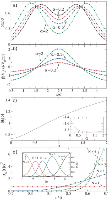
βVi r =βV i− r −lnρr +ln P−ρμ r, n Nn 1 1 n (8) which can be derived from inserting equation (3) into (7) and then inverting with (5). The terms in the sum in equation (8) are re-calculated at each step, using the decomposition proce-dure described above.We first apply the method to a system of one-dimen-sional hard particles, for which the exact grand canonical (Helmholtz) intrinsic free energy functional F[ ]ρμ is known [17]. In order to provide a severe test of the canonical func-tional approach, we consider N = 2 particles of length σ con-fined between two identical hard walls separated by a distance
σ =
h 4.9 along the x-axis. In addition we apply a parabolic external potential V x0( )= −(x h/2)2k TB /σ2. First we find the equilibrium canonical profile ρN 2= ( )x using equation (5). Next, we generate trial density profiles ρα( )x via a multipli-cative perturbation: ρα( )x =A[1+α(x−h/2) ]2 ρN= ( )x
2 ,
where A is a constant that normalizes the profile such that it contains two particles, and α determines the strength of the perturbation, see figure 1(a). The corresponding external potential Vα( )r is then obtained by the iterative method (8). In figure 1(b) we show results for V xα( )−V x0( ) for a range of
values of α. The value of the canonical free energy functional, [ ]ρα
FN , follows from equation (6); the results are plotted in
figure 1(c). As expected, the canonical free energy increases with the perturbation strength α, and it is completely different from the intrinsic Helmholtz grand canonical free energy [17], see the inset of figure 1(c) for F[ ]ρα. Here F[ ]ρα consists of the ideal gas functional and Percus’ excess free-energy functional evaluated at ρα.
In order to demonstrate the applicability of the method to more realistic systems, we consider a three-dimensional case of hard spheres confined in a hard spherical cavity. We employ one of the most advanced free energy functionals presently available, namely the tensorial White Bear II fundamental measure functional [18]. The agreement of the canonical den-sity profiles, as compared to Monte Carlo simulation data, is remarkable, see figure 1(d). The inset of figure 1(d) shows the probabilities pN as a function of μ.
The canonical equilibrium state serves as an initial con-dition for the time evolution. To describe the many-body dynamics, we employ the N-particle Smoluchowski equa-tion [11], which locally conserves the particles throughout the time evolution (no exchange with any particle bath). An exact equation of motion for the time-dependent density
profile ρ r tN( ), is obtained by integrating over N − 1 degrees of freedom, ( ) [ ( ) ( ) ( )( ( ) ( ))] ρ ρ β βρ ∂ ∂ = ∇ ⋅ ∇ − − − ∇ r r r r r r t t D t t t t V t f X , , , , , , , N N N N 0 ext (9)
where D0 is the bare diffusion coefficient, Vext( )r,t is a
time-dependent external potential, X ,( )r t is a non-conservative force field, and f ,N( )r t is the internal force density due to the interparticle interactions. The latter is given exactly by
( ) ( )( ) ( )
∫
ρ = − ′ ′ ∇ | − |′ r t r r r t u r r f ,N d N2 , , (10) where ρ( )N2(r r t, ,′ ) is the exact nonequilibrium pair density for N particles, and u(r) is the interparticle pair potential. Schmidt and Brader [16] have shown that the internal force density can be systematically split into an adiabatic and a superadiabatic contribution,( )r t = ( [ ])r ρ + ( )r t fN , fN , N fN , ,
ad sup
(11) where the adiabatic force density is an instantaneous func-tional of the one-body density distribution and fsupN ( )r t, con-tains memory effects, which are neglected in DDFT. The adiabatic approximation corresponds to setting fsupN ( ) =r t, 0; a fundamental assumption of DDFT, which we retain in the present work. In contrast to DDFT, however, we will treat
( )r
fNad exactly.
The instantaneous nonequilibrium density ρ r tN( ), allows to define at each time t an adiabatic reference state as an equi-librium canonical ensemble of N particles with one-body den-sity distribution
( ) ( )
ρNadr =ρN r t, .
(12) Here the left hand side (as well as all subsequent adiabatic quantities) is in general different at each time. We suppress this time dependence in the notation in order to highlight the static nature of the adiabatic state. The canonical inversion procedure (8) then determines the corresponding external (‘adiabatic’) potential, Vad( )r, which, together with u(r),
speci-fies the adiabatic system completely. Note that Vad( )r is in
general unrelated to Vext( )r,t (as occurring in the equation of motion (9)). The corresponding canonical two-body density distribution ρ( )N2 ad(r r, ′) and the internal force density in the adiabatic system are related by
( ) ( ) ( ) ( )
∫
ρ = − ′ ′∇ | − |′ r r r r u r r fadN d N2 ad , . (13) In the following we demonstrate how fadN( )r can be explicitly calculated. This specifies the adiabatic one-body dynamics completely. We present three different alternatives, all of which yield the same result.(i) As the adiabatic system is in equilibrium, the net force vanishes. Hence the internal forces equal the negative external and entropic forces, and
( )r =ρ ( ) [ ( )r ∇V r +k T ρ ( )]r
fNad adN ad B ln Nad .
(14)
Figure 1. (a) Equilibrium density profile ρN 2= ( )x (solid line)
of a system of N = 2 hard rods confined in a slit pore and in
presence of a parabolic external potential. The dashed lines are trial profiles obtained via ρ( )x =ρN 2( ) [x A1+α(x−h/2) ]2
= for
different perturbation strengths α, as indicated. (b) Difference of scaled external potentials β( ( )V xα −V x0( )) for different values of α. Symbols in (a) and (b) correspond to Monte Carlo simulation,
using the inversion procedure of [15] to obtain V xα( ). (c) Value of the canonical functional βFN 2= and the intrinsic grand canonical free energy functional [17] (inset) evaluated at ρ as a function of the perturbation strength α. (d) Canonical density profiles of hard spheres confined in a spherical cavity of radius r /σ =1.2. The solid lines are obtained via decomposition of the grand canonical functional White Bear mk. II [18]. Symbols represent Monte Carlo simulation data. The inset shows the probabilities pN as a function
Here all quantities on the right hand side are known: the adiabatic density ρ radN( ) via (12), and Vad( )r has already
been obtained from the canonical inversion procedure. (ii) Functional differentiation of the canonical excess (over
ideal gas) free energy functional FexcN [ ]ρ yields
( ) ( ) [ ] ( ) ( ) ( ) ρ δ ρ δρ = − ∇ ρ =ρ r r r F f . r r N N N ad ad exc N ad (15) In practice this procedure requires performing the
func-tional derivative numerically.
(iii) From decomposition of the force in an adiabatic grand canonical state one obtains
( )=
∑
ρ ( )∇ ( )( ) μ μ − r k T r c r fN P , n Nn ad B 1 n 1n (16) where ρμad( )rn is a set of grand canonical density
pro-files in the adiabatic potential Vad( )r, and c( )μ1n( )r are the
corresp onding one-body direct correlation functions. Equation (16) can be derived from the exact grand canonical sum rule
( ) ( )( )
∫
( ) ( ) ( )ρμ r ∇ μ r = − r′ρμ r r′∇ | − |r r′
k TB c1 d 2 ad , u ,
(17) and decomposing the grand canonical two-body density
( ) ( )
ρμ2 adr r, ′ in the adiabatic system.
We have explicitly verified that the three methods yield the same results within numerical accuracy.
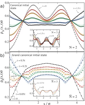
We are now in a position to integrate equation (9) in time using purely canonical forces to drive the dynamics. The adi-abatic potential is re-calculated at each time step. In figure 2(a) we show results from the particle conserving theory for the relaxation of N = 2 and N = 3 (inset) hard rods, following the switching-off of a harmonic potential. The rods remain confined between two hard walls for all times and each system relaxes to its final (canonical) equilibrium state. The theor etical results are in very good agreement with our Brownian Dynamics simula-tion results (simulasimula-tion details can be found in [15]).
The theoretical time evolution is slightly ahead of the simulation data. This is consistent with the direction of the super-adiabatic forces, which we have obtained by simula-tions, following the method of [15]; these results will be pre-sented elsewhere. For the dense state N = 4 we also find very good agreement of theoretical results and simulation data (not shown). Any systematic deviations of theoretical results from the simulation data are entirely due to the omission of super-adiabatic forces in the theory, and not due to ensemble differ-ences. For N = 1 the theory is exact, as the super-adiabatic forces vanish.
It is now straightforward to generalize to grand canonical initial conditions. Let the system at the initial time t = 0 be specified by a grand canonical density distribution ρ( )μ0( )r with average number of particles N = ∑NN p( )N0( )μ. This state can be viewed as being composed of a set of underlying canonical density profiles ρ r( )N0( ) with statistical weights p( )N0( )μ. Each of these canonical states evolves in time under particle con-serving dynamics. Hence the entire grand canonical initial state evolves as a superposition of the trajectories ρN(r t, >0). The statistical weights, however, are those of the initial grand canonical state, p( )N0( )μ, as the system is decoupled from any particle bath for t > 0 (there is no source term in (9)). Hence the one-body density of this system is given by
( )
∑
( )( ) ( ) ρN r,t = p μ ρ r, .t N N N 0 (18) Figure 2(b) shows corresponding results for N =2 and =N 3 (inset). We find again very good agreement between the theory and BD simulation data. The theoretical time
Figure 2. (a) Time evolution of canonical density profiles for a system of N = 2 and N = 3 (inset) particles in one dimension
confined to a slit of width h=4.9σ. For t < 0 the external potential
consists of a harmonic trap Vext( )x = −(x h/2)2k TB /σ2 and hard walls at x = 0 and x/σ =4.9 (such that the density is cut at
x/σ =0.5 and 4.4). At t = 0 the harmonic trap is switched off and
the density relaxes. The density at t = 0 and t=1.5τ are given by the dashed lines, as indicated; the time scale is 2/D
0 τ=σ . At t=1.5τ the system has practically relaxed to the final equilibrium state. Intermediate nonequilibrium profiles are shown at times
t/τ =0.05, 0.10, 0.20, 0.40 (for N = 2) and t/τ =0.05, 0.10, 0.15 (for N = 3) and are given by the full lines. Symbols indicate the
results of Brownian dynamics simulations. (b) Same as panel (a), but for an initial grand canonical profile with average number of particles is N = , according to DDFT (dashed lines), the 2 particle conserving theory (solid lines) and Brownian dynamics simulation (symbols). Solid lines and symbols have been obtained by recomposition of canonical states according to equation (18). The initial state, for t = 0, is the same in all cases. At t=0.5τ the system has almost relaxed to its final state. The inset in (b) shows the time evolution according to DDFT of a grand canonical profile with N = .3
evolution is slightly ahead of the BD data, which is entirely due to having neglected super-adiabatic forces in the theory. The theory captures the correct long-time limit. The time evolution of these initially grand canonical states differs very significantly from that of the corresponding canonical initial states, shown in figure 2(a). This striking discrepancy occurs despite the fact that N =N, which highlights the importance of correct choice of ensemble in finite systems.
We next compare our approach to DDFT. As demonstrated by Archer and Evans [11], DDFT amounts to employing the equilibrium sum rule (17) for expressing the interaction force in terms of the one-body direct correlation function in the grand ensemble. However, instead of using the correct rela-tion (12), DDFT amounts to constructing a grand canonical adiabatic state, with density distribution
( ) ( )
ρμadr =ρN r t, .
(19) Via the Euler–Lagrange equation (7), a corresponding external potential exists, that generates ρμad( )r in the grand ensemble. The grand canonical adiabatic system under the influence of this external potential possess a two-body density, ρ( )μ2(r r, ′), for which using the sum rule (17) yields the associated force density
( )r = −k Tρμ( )r ∇c( )μ ( )r
fDDFT B ad 1 ,
(20) which differs from the exact expression (16). In the example of figure 2(b), although DDFT deviates more strongly from the simulation data than the present theory, it nevertheless pro-vides a reasonable description of the dynamics of an initial grand canonical state.
Although we have presented results for very simple test cases, the particle conserving dynamical theory is applicable to any system for which a grand canonical density functional is available. Studies of complex phenomena, such as the dynamics of colloidal cluster formation, or transport through ion channels are thus within reach. As exemplified by the comparison of figures 2(a) and (b), the time evolution of a system containing only a few particles is very sensitive to the choice of ensemble. In systems with a reduced number of particles the use of a canonical DFT and particle conserving dynamics is indispensable in order to compare with experi-ments or simulations performed at fixed particle number. Canonical and grand canonical ensembles are equivalent in the thermodynamic limit, and the time evolution in DFT is just a temporal sequence of equilibrium states. Hence, one might expect our particle conserving theory and (standard) DDFT to be equivalent in systems with a large number of particles. However, local fluctuations typically involve only a reduced number of particles. Therefore, the dynamics of localized phenomena might depend on the ensemble, even
in the thermodynamic limit. This is an open problem to be addressed in future work.
Acknowledgments
DdlH and JMB contributed equally to this work.
References
[1] Evans R 1979 The nature of the liquid-vapour interface and other topics in the statistical mechanics of non-uniform, classical fluids Adv. Phys. 28 143–200
[2] Mermin N D 1965 Thermal properties of the inhomogeneous electron gas Phys. Rev. 137 A1441
[3] Meng G, Arkus N, Brenner M P and Manoharan V N 2010
Science 327 560
[4] González A, White J A, Román F L, Velasco S and Evans R 1997 Density functional theory for small systems: hard spheres in a closed spherical cavity Phys. Rev. Lett.
79 2466
[5] White J A, González A, Román F L and Velasco S 2000 Density-functional theory of inhomogeneous fluids in the canonical ensemble Phys. Rev. Lett. 84 1220
[6] de las Heras D and Schmidt M 2014 Full canonical
information from grand-potential density-functional theory
Phys. Rev. Lett. 113 238304
[7] Chakraborty D, Dufty J and Karasiev V V 2015 System-size dependence in grand canonical and canonical ensembles
Adv. Quant. Chem. 71 11
[8] Hernando J A and Blum L 2001 Density functional formalism in the canonical ensemble J. Phys.: Condens. Matter
13 L577
[9] Dwandaru W S B and Schmidt M 2011 Variational principle of classical density functional theory via Levy’s constrained search method Phys. Rev. E 83 061133
[10] Marconi U M B and Tarazona P 1999 Dynamic density functional theory of fluids J. Chem. Phys. 110 8032
[11] Archer A J and Evans R 2004 Dynamical density functional theory and its application to spinodal decomposition
J. Chem. Phys. 121 4246
[12] Penna F, Dzubiella J and Tarazona P 2003 Dynamic density functional study of a driven colloidal particle in polymer solutions Phys. Rev. E 68 061407
[13] Dzubiella J and Likos C N 2003 Mean-field dynamical density functional theory J. Phys.: Condens. Matter 15 L147
[14] Royall C P, Dzubiella J, Schmidt M and van Blaaderen A 2007 Nonequilibrium sedimentation of colloids on the particle scale Phys. Rev. Lett. 98 188304
[15] Fortini A, de las Heras D, Brader J M and Schmidt M 2014 Superadiabatic forces in Brownian many-body dynamics
Phys. Rev. Lett. 113 167801
[16] Schmidt M and Brader J M 2013 Power functional theory for Brownian dynamics J. Chem. Phys. 138 214101
[17] Percus J K 1976 Equilibrium state of a classical fluid of hard rods in an external field J. Stat. Phys. 15 505
[18] Hansen-Goos H and Roth R 2006 Density functional theory for hard-sphere mixtures: the White Bear version mark II