Sparse stabilization and control of the Cucker-Smale model

HAL Id: hal-00743792

https://hal.archives-ouvertes.fr/hal-00743792

HAL is a multi-disciplinary open access

archive for the deposit and dissemination of sci-entific research documents, whether they are pub-lished or not. The documents may come from teaching and research institutions in France or

L’archive ouverte pluridisciplinaire HAL, est destinée au dépôt et à la diffusion de documents scientifiques de niveau recherche, publiés ou non, émanant des établissements d’enseignement et de recherche français ou étrangers, des laboratoires

Sparse stabilization and control of the Cucker-Smale

model

Marco Caponigro, Massimo Fornasier, Benedetto Piccoli, Emmanuel Trélat

To cite this version:

Marco Caponigro, Massimo Fornasier, Benedetto Piccoli, Emmanuel Trélat. Sparse stabilization and control of the Cucker-Smale model. Mathematical Models and Methods in Applied Sciences, World Scientific Publishing, 2015, 25 (3), pp.521–564. �hal-00743792�

Sparse Stabilization and Control of the Cucker-Smale Model

Marco Caponigro∗, Massimo Fornasier†, Benedetto Piccoli‡, Emmanuel Tr´elat§ October 19, 2012

Abstract

From a mathematical point of view self-organization can be described as patterns to which certain dynamical systems modeling social dynamics tend spontaneously to be attracted. In this paper we explore situations beyond self-organization, in particular how to externally control such dynamical systems in order to eventually enforce pattern formation also in those situations where this wished phenomenon does not result from spontaneous convergence. Our focus is on dynamical systems of Cucker-Smale type, modeling consensus emergence, and we question the existence of stabilization and optimal control strategies which require the minimal amount of external interven-tion for nevertheless inducing consensus in a group of interacting agents. First we follow a greedy approach, by designing instantaneous feedback controls with two different sparsity properties: com-ponentwise sparsity, meaning that the controls have at most one nonzero component at every instant

of time and their implementation is based on a variational criterion involving ℓ1-norm penalization

terms; time sparsity, meaning that the number of switchings is bounded on every compact interval of time, and such controls are realized by means of a sample-and-hold procedure. Controls sharing these two sparsity features are very realistic and convenient for practical issues. Moreover we show that among the controls built out of the mentioned variational principle, the maximally sparse ones are instantaneously optimal in terms of the decay rate of a suitably designed Lyapunov functional, measuring the distance from consensus. As a consequence we provide a mathematical justification to the general principle according to which “sparse is better” in the sense that a policy maker, who is not allowed to predict future developments, should always consider more favorable to intervene with stronger action on the fewest possible instantaneous optimal leaders rather than trying to control more agents with minor strength in order to achieve group consensus. We then establish local and global sparse controllability properties to consensus. Finally, we analyze the sparsity of solutions of the finite time optimal control problem where the minimization criterion is a

combina-tion of the distance from consensus and of the ℓ1-norm of the control. Such an optimization models

the situation where the policy maker is actually allowed to observe future developments. We show that the lacunarity of sparsity is related to the codimension of certain manifolds in the space of cotangent vectors.

Keywords: Cucker-Smale model, consensus emergence, ℓ1-norm minimization, optimal complexity, sparse stabilization, sparse optimal control.

MSC 2010: 34D45, 35B36, 49J15, 65K10, 93D15, 93B05

∗_{Conservatoire National des Arts et M´etiers, D´epartement Ing´enierie Math´ematique (IMATH), ´Equipe M2N, 292 rue} Saint-Martin, 75003, Paris, France. (marco.caponigro@cnam.fr)

†_{Technische Universit¨at M¨unchen, Facult¨at Mathematik, Boltzmannstrasse 3 D-85748, Garching bei M¨unchen,} Ger-many (massimo.fornasier@ma.tum.de).

‡_{Rutgers University, Department of Mathematics, Business & Science Building Room 325 Camden, NJ 08102, USA} (piccoli@camden.rutgers.edu).

§_{Universit´e Pierre et Marie Curie (Univ. Paris 6) and Institut Universitaire de France, CNRS UMR 7598, Laboratoire} Jacques-Louis Lions, F-75005, Paris, France (emmanuel.trelat@upmc.fr).

Contents

1 Introduction 2

1.1 Self-organization Vs organization via intervention . . . 2

1.2 The general Cucker-Smale model and introduction to its control . . . 4

2 Sparse Feedback Control of the Cucker-Smale Model 9 2.1 A first result of stabilization . . . 9

2.2 Componentwise sparse feedback stabilization . . . 9

2.3 Time sparse feedback stabilization . . . 13

2.4 Componentwise sparse selections are absolutely continuous solutions . . . 16

3 Sparse is Better 17 3.1 Instantaneous optimality of componentwise sparse controls . . . 17

3.2 Complexity of consensus . . . 21

4 Sparse Controllability Near the Consensus Manifold 22 5 Sparse Optimal Control of the Cucker-Smale Model 24 6 Appendix 27 6.1 Proof of Lemma 1 . . . 27

6.2 Proof of Proposition 1 . . . 27

6.3 A technical Lemma . . . 29

1

Introduction

1.1 Self-organization Vs organization via intervention

In recent years there has been a very fast growing interest in defining and analyzing mathematical models of multiple interacting agents in social dynamics. Usually individual based models, described by suitable dynamical systems, constitute the basis for developing continuum descriptions of the agent distribution, governed by suitable partial differential equations. There are many inspiring applications, such as animal behavior, where the coordinated movement of groups, such as birds (starlings, geese, etc.), fishes (tuna, capelin, etc.), insects (locusts, ants, bees, termites, etc.) or certain mammals (wilde-beasts, sheep, etc.) is considered, see, e.g., [2, 6, 18, 19, 45, 48, 49, 56, 63, 65] or the review chapter [8], and the numerous references therein. Models in microbiology, such as the Patlak-Keller-Segel model [39, 50], describing the chemotactical aggregation of cells and multicellular micro-organisms, inspired a very rich mathematical literature [35, 36, 52], see also the very recent work [4] and references therein. Human motion, including pedestrian and crowd modeling [21, 22], for instance in evacuation process simulations, has been a matter of intensive research, connecting also with new developments such as mean field games, see [40] and the overview in its Section 2. Certain aspects of human social behav-ior, as in language evolution [23, 25, 38] or even criminal activities [58], are also subject of intensive study by means of dynamical systems and kinetic models. Moreover, relevant results appeared in the economical realm with the theoretical derivation of wealth distributions [27] and, again in connection with game theory, the description of formation of volatility in financial markets [41]. Beside applica-tions where biological agents, animals and micro-(multi)cellular organisms, or humans are involved, also more abstract modeling of interacting automatic units, for instance simple robots, are of high practical interest [11, 37, 61, 42, 51, 57].

One of the leading concepts behind the modeling of multiagent interaction in the past few years has been self-organization [6, 45, 48, 49, 63], which, from a mathematical point of view, can be described as the formation of patterns, to which the systems tend naturally to be attracted. The fascinating mechanism to be revealed by such a modeling is how to connect the microscopical and usually binary rules or social forces of interaction between individuals with the eventual global behavior or group pattern, forming as a superposition in time of the different microscopical effects. Hence, one of the interesting issues of such socio-dynamical models is the global convergence to stable patterns or, as more often and more realistically, the instabilities and local convergence [52].

While the description of pattern formation can explain some relevant real-life behaviors, it is also of paramount interest how one may enforce and stabilize pattern formation in those situations where global and stable convergence cannot be ensured, especially in presence of noise [68], or, vice versa, how one can avoid certain rare and dangerous patterns to form, despite that the system may suddenly tend stably to them. The latter situations may refer, for instance, to the so-called “black swans”, usually referred to critical (financial or social) events [3, 62]. In all these situations where the inde-pendent behavior of the system, despite its natural tendencies, does not realize the desired result, the active intervention of an external policy maker is essential. This naturally raises the question of which optimal policy should be considered.

In information theory, the best possible way of representing data is usually the most economical for re-liably or robustly storing and communicating data. One of the modern ways of describing economical description of data is their sparse representation with respect to an adapted dictionary [43, Chapter 1]. In this paper we shall translate these concepts to realize best policies in stabilization and control of dynamical systems modeling multiagent interactions. Beside stabilization strategies in collective behavior already considered in the recent literature, see e.g. [55, 57], the conceptually closest work to our approach is perhaps the seminal paper [42], where externally driven “virtual leaders” are inserted in a collective motion dynamics in order to enforce a certain behavior. Nevertheless our modeling still differs significantly from this mentioned literature, because we allow us directly, externally, and instantaneously to control the individuals of the group, with no need of introducing predetermined virtual leaders, and we shall specifically seek for the most economical (sparsest) way of leading the group to a certain behavior. In particular, we will mathematically model sparse controls, designed to promote the minimal amount of intervention of an external policy maker, in order to enforce nev-ertheless the formation of certain interesting patterns. In other words we shall activate in time the minimal amount of parameters, potentially limited to certain admissible classes, which can provide a certain verifiable outcome of our system. The relationship between parameter choices and result will be usually highly nonlinear, especially for several known dynamical system, modeling social dynamics. Were this relationship linear instead, then a rather well-established theory predicts how many degrees of freedom are minimally necessary to achieve the expected outcome, and, depending on certain spec-tral properties of the linear model, allows also for efficient algorithms to compute them. This theory is known in mathematical signal processing under the name of compressed sensing, see the seminal work [7] and [26], see also the review chapter [30]. The major contribution of these papers was to re-alize that one can combine the power of convex optimization, in particular ℓ1-norm minimization, and spectral properties of random linear models in order to show optimal results on the ability of ℓ1-norm minimization of recovering robustly sparsest solutions. Borrowing a leaf from compressed sensing, we will model sparse stabilization and control strategies by penalizing the class of vector valued controls u = (u1, . . . , uN) ∈ (Rd)N by means of a mixed ℓN1 − ℓd2-norm, i.e.,

N X

i=1 kuik,

where here k · k is the ℓd2-Euclidean norm on Rd. This mixed norm has been used for instance in [29] as a joint sparsity constraint and it has the effect of optimally sparsifying multivariate vectors in compressed sensing problems [28]. The use of (scalar) ℓ1-norms to penalize controls dates back to the 60’s with the models of linear fuel consumption [20]. More recent work in dynamical systems [66] resumes again ℓ1-minimization emphasizing its sparsifying power. Also in optimal control with partial differential equation constraints it became rather popular to use L1-minimization to enforce sparsity of controls [9, 13, 14, 34, 53, 60, 67].

Differently from this previously mentioned work, we will investigate in this paper optimally sparse stabilization and control to enforce pattern formation or, more precisely, convergence to attractors in dynamical systems modeling multiagent interaction. A simple, but still rather interesting and prototypical situation is given by the individual based particle system we are considering here as a particular case        ˙xi = vi ˙vi = 1 N N X j=1 vj− vi (1 + kxj− xik2₎β (1)

for i = 1, . . . , N , where β > 0 and xi _{∈ R}d, vi _{∈ R}dare the state and consensus parameters respectively. Here one may want to imagine that the vis actually represent abstract quantities such as words of a communication language, opinions, invested capitals, preferences, but also more classical physical quantities such as the velocities in a collective motion dynamics. This model describes the emerging of consensus in a group of N interacting agents described by 2d degrees of freedom each, trying to align (also in terms of abstract consensus) with their social neighbors. One of the motivations of this model proposed by Cucker and Smale was in fact to describe the formation and evolution of languages [23, Section 6], although, due to its simplicity, it has been eventually related mainly to the description of the emergence of consensus in a group of moving agents, for instance flocking in a swarm of birds [24]. One of the interesting features of this simple system is its rather complete analytical description in terms of its ability of convergence to attractors according to the parameter β > 0 which is ruling the communication rate between far distant agents. For β 6 1₂, corresponding to a still rather strong long - social - distance interaction, for every initial condition the system will converge to a consensus pattern, characterized by the fact that all the parameters v_{i(t)s will tend for t → +∞ to} the mean ¯v = _N1 PN_i=1vi(t) which is actually an invariant of the dynamics. For β > 1₂, the emergence of consensus happens only under certain concentration conditions in state and consensus parameters, i.e., when the group is sufficiently close to its state center of mass or when the consensus parameters are sufficiently close to their mean. Nothing instead can be said a priori when at the same time one has β > 1₂ and the mentioned concentration conditions are not provided. Actually one can easily construct counterexamples to formation of consensus, see our Example 1 below. In this situation, it is interesting to consider external control strategies which will facilitate the formation of consensus, which is precisely the scope of this work.

1.2 The general Cucker-Smale model and introduction to its control

Let us introduce the more general Cucker-Smale model under consideration in this article.

The model. We consider a system of N interacting agents. The state of each agent is described by a pair (xi, vi) of vectors of the Euclidean space Rd, where xi represents the main state of an agent and the vi its consensus parameter. The main state of the group of N agents is given by the N -uple x = (x1, . . . , xN). Similarly for the consensus parameters v = (v1, . . . , vN). The space of main states

and the space of consensus parameters is (Rd)N for both, the product N -times of the Euclidean space Rd _{endowed with the induced inner product structure.}

The time evolution of the state (xi, vi) of the ith agent is governed by the equations        ˙xi(t) = vi(t), ˙vi(t) = 1 N N X j=1 a(kxj(t) − xi(t)k)(vj(t) − vi(t)), (2)

for every i = 1, . . . , N , where a ∈ C1_{([0, +∞)) is a nonincreasing positive function. Here, k · k denotes} again the ℓd₂-Euclidean norm in Rd. The meaning of the second equation is that each agent adjusts its consensus parameter with those of other agents in relation with a weighted average of the differences. The influence of the jth_{agent on the dynamics of the i}th _{is a function of the (social) distance of the two} agents. Note that the mean consensus parameter ¯v = _N1 PN_i=1vi(t) is an invariant of the dynamics, hence it is constant in time.

As mentioned previously, an example of a system of the form (2) is the influential model of Cucker and Smale [23] in which the function a is of the form

a(kxj− xik) = K (σ2_{+ kx}

i− xjk2)β

, (3)

where K > 0, σ > 0, and β > 0 are constants accounting for the social properties of the group of agents.

In matrix notation, System (2) can be written as (

˙x = v

˙v = −Lxv, (4)

where Lx is the Laplacian1 _{of the N × N matrix (a(kx}j− xik)/N)N_i,j=1 and depends on x. The Laplacian Lx is an N × N matrix acting on (Rd)N, and verifies Lx(v, . . . , v) = 0 for every v ∈ Rd. Notice that the operator Lx always is positive semidefinite.

Consensus. _{For every v ∈ (R}d)N_{, we define the mean vector ¯v =} 1 N

PN

i=1vi and the symmetric bilinear form B on (Rd)N _{× (R}d)N by B(u, v) = 1 2N2 N X i,j=1 hui− uj, vi− vji = 1 N N X i=1

hui, vii − h¯u, ¯vi, where h·, ·i denotes the scalar product in Rd. We set

Vf = {(v1, . . . , vN) ∈ (Rd)N | v1 = · · · = vN ∈ Rd}, (5) V⊥= {(v1, . . . , vN_{) ∈ (R}d)N _| N X i=1 vi _{= 0}.} (6)

These are two orthogonal subspaces of (Rd)N_{. Every v ∈ (R}d)N can be written as v = vf + v⊥ with vf = (¯v, . . . , ¯v) ∈ Vf and v⊥ ∈ V⊥.

1_{Given a real N × N matrix A = (aij)i,j and v ∈ (R}d₎N _{we denote by Av the action of A on (R}d₎N _{by mapping v} to (ai1v1+ · · · + aiNvN)i=1,...,N. Given a nonnegative symmetric N × N matrix A = (aij)i,j, the Laplacian L of A is defined by L = D − A, with D = diag(d1, . . . , dN) and dk=PN_j=1akj.

Note that B restricted to V⊥× V⊥ coincides, up to the factor 1/N , with the scalar product on (Rd₎N_{. Moreover B(u, v) = B(u}

⊥, v) = B(u, v⊥) = B(u⊥, v⊥). Indeed B(u, vf) = 0 = B(uf, v) for every u, v ∈ (Rd₎N_.

Given a solution (x(t), v(t)) of (2) we define the quantities X(t) := B(x(t), x(t)) = 1 2N2 N X i,j=1 kxi(t) − xj(t)k2, and V (t) := B(v(t), v(t)) = 1 2N2 N X i,j=1 kvi(t) − vj(t)k2= 1 N N X i=1 kv(t)⊥ik 2_.

Consensus is a state in which all agents have the same consensus parameter.

Definition 1 _{(Consensus point). A steady configuration of System (2) (x, v) ∈ (R}d)N _{× Vf} is called a consensus point in the sense that the dynamics originating from (x, v) is simply given by rigid translation x(t) = x + t¯v. We call (Rd₎N _{× Vf is the consensus manifold.}

Definition 2 (Consensus). We say that a solution (x(t), v(t)) of System (2) tends to consensus if the consensus parameter vectors tend to the mean ¯v = _N1 P_ivi, namely if limt→∞vi(t) = ¯v for every i = 1, . . . , N .

Remark 1. Because of uniqueness, a solution of (2) cannot reach consensus within finite time, unless the initial datum is already a consensus point. The consensus manifold is invariant for (2).

Remark 2. The following definitions of consensus are equivalent: (i) lim_t→∞vi(t) = ¯v for every i = 1, . . . , N ;

(ii) lim_t→∞v_⊥i(t) = 0 for every i = 1, . . . , N ;

(iii) lim_t→∞V (t) = 0.

The following lemma, whose proof is given in the Appendix, shows that actually V (t) is a Lyapunov functional for the dynamics of (2).

Lemma 1. For every t > 0

d

dtV (t) 6 −2a ³p

2N X(t)´V (t). In particular if sup_t>0X(t) 6 ¯X then lim_t→∞V (t) = 0.

For multi-agent systems of the form (2) sufficient conditions for consensus emergence are a partic-ular case of the main result of [32] and are summarized in the following proposition, whose proof is recalled in the Appendix, for self-containedness and reader’s convenience.

Proposition 1. Let (x0, v0) ∈ (Rd)N × (Rd)N be such that X0 = B(x0, v0) and V0 = B(x0, v0) satisfy Z _∞

√ X0

a(√2N r)dr >pV0. (7) Then the solution of (2) with initial data (x0, v0) tends to consensus.

In the following we call the subset of (Rd)N _{× (R}d)N satisfying (7) the consensus region, which represents the basin of attraction of the consensus manifold. Notice that the condition (7) is actually satisfied as soon as V0 and X0are sufficiently small, i.e., the system has initially sufficient concentration in the consensus parameters and in the main states.

Although consensus forms a rigidly translating stable pattern for the system and represents in some sense a “convenient” choice for the group, there are initial conditions for which the system does not tend to consensus, as the following example shows.

Example 1(Cucker–Smale system: two agents on the line). Consider the Cucker–Smale system (2)-(3) in the case of two agents moving on R with position and velocity at time t, (x1(t), v1(t)) and (x2(t), v2(t)). Assume for simplicity that β = 1, K = 2, and σ = 1. Let x(t) = x1_{(t) − x}2(t) be the relative main state and v(t) = v1(t) − v2(t) be the relative consensus parameter. Equation (2), then

reads _



 ˙x = v ˙v = −_{1 + x}v ₂

with initial conditions x(0) = x0 and v(0) = v0> 0. The solution of this system can be found by direct integration, as from ˙v = − ˙x/(1 + x2) we have

v(t) − v0 = − arctan x(t) + arctan x0.

If the initial conditions satisfy arctan x0 + v0 < π/2 then the relative main state x(t) is bounded uniformly by tan (arctan x0+ v0), satisfying the sufficient boundedness condition on the space variables in Lemma 1 for consensus.

On the other hand, whenever arctan x0+ v0 > π/2, which implies arctan x0 + v0 > π/2 + ε for some ε > 0, the consensus parameter v(t) remains bounded away from 0 for every time, since

v(t) = − arctan x(t) + arctan x0+ v0>π/2 − arctan x(t) + ε > ε > 0, for every t > 0. In other words, the system does not tend to consensus.

Control of the Cucker-Smale model. When the consensus in a group of agents is not achieved by self-organization of the group, as in Example 1, it is natural to ask whether it is possible to induce the group to reach it by means of an external action. In this sense we introduce the notion of organization via intervention. We consider the system (2) of N interacting agents, in which the dynamics of every agent are moreover subject to the action of an external field. Admissible controls, accounting for the external field, are measurable functions u = (u1, . . . , uN_{) : [0, +∞) → (R}d)N satisfying the ℓN_{1 − ℓ}d₂-norm constraint

N X

i=1

kui(t)k 6 M, (8)

for every t > 0, for a given positive constant M . The time evolution of the state is governed by        ˙xi(t) = vi(t), ˙vi(t) = 1 N N X j=1 a(kxj(t) − xi(t)k)(vj(t) − vi(t)) + ui(t), (9)

for i = 1, . . . , N , and xi ∈ Rd, vi ∈ Rd. In matrix notation, the above system can be written as (

˙x = v

where Lx is the Laplacian defined in Section 1.2.

Our aim is then to find admissible controls steering the system to the consensus region in finite time. In particular, we shall address the question of quantifying the minimal amount of intervention one external policy maker should use on the system in order to lead it to consensus, and we formulate a practical strategy to approach optimal interventions.

Our first approach will be a greedy one, in the sense that we will design a feedback control which will optimize instantaneously three fundamental quantities:

(i) it has the minimal amount of components active at each time;

(ii) it has the minimal amount of switchings equispaced in time within the finite time interval to reach the consensus region;

(iii) it maximizes at each switching time the rate of decay of the Lyapunov functional measuring the distance to the consensus region.

This approach models the situation where the external policy maker is actually not allowed to predict future developments and has to make optimal decisions based on instantaneous configurations. Note that a componentwise sparse feedback control as in (i) is more realistic and convenient in practice than a control simultaneously active on more or even all agents, because it requires acting only on at most one agent, at every instant of time. The adaptive and instantaneous rule of choice of the controls is based on a variational criterion involving ℓN_{1 − ℓ}d₂-norm penalization terms. Since however such componentwise sparse controls are likely to be chattering, i.e., requiring an infinite number of changes of the active control component over a bounded interval of time, we will also have to pay attention in deriving control strategies with property (ii), which are as well sparse in time, and we therefore call them time sparse controls.

Our second approach is based on a finite time optimal control problem where the minimization crite-rion is a combination of the distance from consensus and of the ℓN_{1 − ℓ}d₂-norm of the control. Such an optimization models the situation where the policy maker is actually allowed to make deterministic future predictions of the development. We show that componentwise sparse solutions are again likely to be the most favorable.

The rest of the paper is organized as follows: Section 2 is devoted to establishing sparse feedback controls stabilizing System (9) to consensus. We investigate the construction of componentwise and time sparse controls. In Section 3 we discuss in which sense the proposed sparse feedback controls have actually optimality properties and we address a general notion of complexity for consensus problems. In Section 4 we we combine the results of the previous sections with a local controllability result near the consensus manifold in order to prove global sparse controllability of Cucker-Smale consensus models. We study the sparsity features of solutions of a finite time optimal control of Cucker-Smale consensus models in Section 5 and we establish that the lacunarity of their sparsity is related to the codimension of certain manifolds. The paper is concluded by an Appendix which collects some of the merely technical results of the paper.

2

Sparse Feedback Control of the Cucker-Smale Model

2.1 A first result of stabilization

Note first that if the integral R₀∞a(r)dr diverges then every pair (X, V ) > 0 satisfies (7), in other words the interaction between the agents is so strong that the system will reach the consensus no matter what the initial conditions are. In this section we are interested in the case where consensus does not arise autonomously therefore throughout this section we will assume that

a ∈ L1(0, +∞).

As already clarified in Lemma 1 the quantity V (t) is actually a Lyapunov functional for the uncon-trolled System (2). For the conuncon-trolled System (9) such quantity actually becomes dependent on the choice of the control, which can nevertheless be properly optimized. As a first relevant and instructive observation we prove that an appropriate choice of the control law can always stabilize the system to consensus.

Proposition 2. For every M > 0 and initial condition (x0, v0) ∈ (Rd)N× (Rd)N, the feedback control defined pointwise in time by u(t) = −αv⊥(t), with 0 < α 6 M

N√B(v0,v0), satisfies the constraint (8) for

every t > 0 and stabilizes the system (9) to consensus in infinite time.

Proof. Consider the solution of (9) with initial data (x0, v0) associated with the feedback control u = −αv⊥, with 0 < α 6 M N√B(v0,v0). Then, by non-negativity of Lx, d dtV (t) = d dtB(v(t), v(t)) = −2B(Lxv(t), v(t)) + 2B(u(t), v(t)) 62B(u(t), v(t)) = −2αB(v⊥(t), v_⊥(t)) = −2αV (t).

Therefore V (t) 6 e−2αt_{V (0) and V (t) tends to 0 exponentially fast as t → ∞. Moreover} N X i=1 kui(t)k 6 √ N v u u t N X i=1 kui(t)k2 = α √ N v u u t N X i=1 kv⊥i(t)k2 = αN p V (t) 6 αNpV (0) = M, and thus the control is admissible.

In other words the system (8)-(9) is semi-globally feedback stabilizable. Nevertheless this result has a merely theoretical value: the feedback stabilizer u = −αv⊥ is not convenient for practical purposes since it requires to act at every instant of time on all the agents in order to steer the system to consensus, which may require a large amount of instantaneous communications. In what follows we address the design of more economical and practical feedback controls which can be both componentwise and time sparse.

2.2 Componentwise sparse feedback stabilization

Definition 3. _{For every M > 0 and every (x, v) ∈ (R}d)N _{× (R}d)N, let U (x, v) be defined as the set of solutions of the variational problem

min à B(v, u) + γ(B(x, x)) N X i=1 kuik ! subject to N X i=1 kuik 6 M , (11) where γ(X) = Z _∞ √ X a(√2N r)dr. (12)

The meaning of (11) is the following. Minimizing the component B(v, u) = B(v_⊥, u) means that, at every instant of time, the control u ∈ U(x, v) is of the form u = −α · v⊥, for some α = (α1, . . . , αN) sequence of nonnegative scalars. Hence it acts as an additional force which pulls the particles towards having the same mean consensus parameter. Imposing additional ℓN_{1 − ℓ}d₂-norm constraints has the function of enforcing sparsity, i.e., most of the α′_is will turn out to be zero, as we will in more detail clarify below. Eventually, the threshold γ(X) is chosen in such a way that the control switches-off as soon as the criterion (7) gets fulfilled.

The componentwise sparsity feature of feedback controls u(x, v) ∈ U(x, v) is analyzed in the next remark, where we make explicit the set U (x, v) according to the value of (x, v) in a partition of the space (Rd)N_{× (R}d)N.

Remark 3. _{First of all, it is easy to see that, for every (x, v) ∈ (R}d)N _{× (R}d₎N _{and every element} u(x, v) ∈ U(x, v) there exist nonnegative real numbers αis such that

ui(x, v) =    0 if v_⊥i = 0, − αi v⊥i kv⊥ik if v_{⊥i 6= 0,} (13) where 0 6PN_i=1αi 6M .

The componentwise sparsity of u depends on the possible values that the αi’s may take in function of (x, v). Actually, the space (Rd)N_{× (R}d)N can be partitioned in the union of the four disjoint subsets C1, C2, C3, and C4 defined by

C1 = {(x, v) ∈ (Rd₎N _{× (R}d₎N _{| B(v, v) < γ(B(x, x))}2_}, C2 = {(x, v) ∈ (Rd)N _{× (R}d)N _{| B(v, v) = γ(B(x, x))}2_},

C3 = {(x, v) ∈ (Rd)N × (Rd)N | B(v, v) > γ(B(x, x))2, and there exists a unique i ∈ {1, . . . , N} such that kv⊥ik > kv⊥jk for every j 6= i},

C4 = {(x, v) ∈ (Rd₎N_×(Rd₎N _{| B(v, v) > γ(B(x, x))}2_{and there exist k > 2 and i}

1, . . . , ik ∈ {1, . . . , N} such that kv⊥i1k = · · · = kv⊥ikk and kv⊥i1k > kv⊥jk for every j /∈ {i1, . . . , ik}}.

The subsets C1 and C3 are open, and the complement (C1∪ C3)c has Lebesgue measure zero. Moreover for every (x, v) ∈ C1∪C3, the set U (x, v) is single valued and its value is a sparse vector with at most one nonzero component. More precisely, one has U |C1 = {0} and U|C3 = {(0, . . . , 0, −Mv⊥i/kv⊥ik, 0, . . . , 0)}

for some unique i ∈ {1, . . . , N}.

If (x, v) ∈ C2∪ C4 then a control in U (x, v) may not be sparse: indeed in these cases the set U (x, v) consists of all u = (u1, . . . , uN) ∈ (Rd)N such that ui= −αiv⊥i/kv⊥ik for every i = 1, . . . , N, where the

αi’s are nonnegative real numbers such that 0 6PN_i=1αi6M whenever (x, v) ∈ C2, andPN_i=1αi = M whenever (x, v) ∈ C4.

By showing that the choice of feedback controls as in Definition 3 optimizes the Lyapunov functional V (t), we can again prove convergence to consensus.

Theorem 1. _{For every (x, v) ∈ (R}d)N _{× (R}d₎N_{, and M > 0, set F (x, v) = {(v, −Lxv + u) | u ∈} U (x, v)}, where U(x, v) is as in Definition 3. Then for every initial datum (x0, v0_{) ∈ (R}d)N _{× (R}d)N, the differential inclusion

( ˙x, ˙v) ∈ F (x, v) (14)

with initial condition (x(0), v(0)) = (x0, v0) is well-posed and its solutions converge to consensus as t tends to +∞.

Remark 4. _{By definition of the feedback controls u(x, v) ∈ U(x, v), and from Remark 3, it follows} that, along a closed-loop trajectory, as soon as V (t) is small enough with respect to γ(B(x, x)) the trajectory has entered the consensus region defined by (7). From this point in time no action is further needed to stabilize the system, since Proposition 1 ensures then that the system is naturally stable to consensus. In particular the control switches-off automatically by being set to 0 forever. It follows from the proof of Theorem 1 below that the time T needed to steer the system to the consensus region is not larger than _MN ³p_{V (0) − γ( ¯}X)´, where γ is defined by (12), and ¯X = 2X(0) +_2MN42V (0)2.

Proof of Theorem 1. First of all we prove that (14) is well-posed, by using general existence results of the theory of differential inclusions (see e.g. [1, Theorem 2.1.3]). For that we address the following steps:

• being the set F (x, v) non-empty, closed, and convex for every (x, v) ∈ (Rd)N _{× (R}d)N (see Remark 3), we show that F (x, v) is upper semi-continuous; this will imply local existence of solutions of (14);

• we will then argue the global extension of these solutions for every t > 0 by the classical theory of ODE’s, as it is sufficient to remark that there exist positive constants c1, c2 such that kF (x, v)k 6 c1kvk + c2.

Let us address the upper semi-continuity of F (x, v), that is for every (x0, v0) and for every ε > 0 there exists δ > 0 such that

F (Bδ(x0, v0)) ⊂ Bε(F (x0, v0)),

where Bδ(y), Bε(y) are the balls of (Rd)N×(Rd)N centered in y with radius δ and ε respectively. As the composition of upper semi-continuous functions is upper semi-continuous (see [1, Proposition 1.1.1]), then it is sufficient to prove that U (x, v) is upper semi continuous. For every (x, v) ∈ C1∪ C3, U (x, v) is single valued and continuous. If (x, v) ∈ C2 then there exist i1, . . . , ik such that kv⊥_i1k = · · · = kv⊥_ikk and kv⊥_i1k > kv⊥lk for every l /∈ {i1, . . . , ik}. If δ < minl /∈{i1,...,ik}

³

kv⊥_i1k − kv⊥lk

´ then U (Bδ(x, v)) = U (x, v) hence, in particular, it is upper semi continuous. With a similar argument it is possible to prove that U (x, v) is upper semi continuous for every (x, v) ∈ C4. This establishes the well-posedness of (14).

Now, let (x(·), v(·)) be a solution of (14). Let T the minimal time needed to reach the consensus, that is T is the smallest number such that V (T ) = γ(X(T ))2_{, with the convention that T = +∞ if the} system does not reach consensus. Let t ∈ (0, T ), then V (t) > γ(X(t))2. Thus the trajectory (x(·), v(·)) is in C3 or C4 and there exist indices i1, . . . , ik in {1, . . . , N} such that kv⊥_i1(t)k = · · · = kv⊥_ik(t)k and kv⊥_i1(t)k > kv⊥j(t)k for every j /∈ {i1, . . . , ik}. Hence if u(t) ∈ U(x(t), v(t)) then

uj(t) =      −αj v_⊥j(t) kv⊥j(t)k if j ∈ {i1, . . . , i_k}, 0 otherwise,

wherePk_j=1αij = M . Then, d dtV (t) = d dtB(v(t), v(t)) 62B(u(t), v(t)) = 2 N N X i=1 hui(t), v_⊥i(t)i = −_N2 k X j=1 αijkv⊥_ij(t)k = −2M Nkv⊥i1(t)k 6₋₂M N p V (t). (15)

For clarity, notice that in the last inequality we used the maximality of kv⊥i1(t)k for which

N N2kv⊥i1(t)k 2 _> 1 N2 N X j=1 kv⊥j(t)k 2_, or √ N N kv⊥i1(t)k > 1 √ N   1 N N X j=1 kv⊥j(t)k 2   1/2 , and eventually −1 Nkv⊥i1(t)k 6 − 1 N p V (t).

Let V0 = V (0) and X0 = X(0). It follows from Lemma 5 in Appendix, or simply by direct integration, that V (t) 6 µ p V0− M Nt ¶2 , (16) and X(t) 6 2X0+ N4 2M2V 2 0 = ¯X.

Note that the time T needed to steer the system in the consensus region is not larger than T0 = N M ³p V0− γ( ¯X) ´ , (17)

and in particular it is finite. Indeed, for every t > T0 we have p

V (t) <pV (T0) 6pV0₋M

NT0= γ( ¯X) 6 γ(X(t)),

and Proposition 1, in particular (7), implies that the system is in the consensus region.

Since we have V (t) = B(v(t), v(t)) < γ(X(t))2 _{for every t > T , it follows that (x(t), v(t)) ∈ C1}, which implies that U (x(t), v(t)) = {0}. Then by Lemma 1 we infer that V (t) tends to 0.

Within the set U (x, v) as in Definition 3, which in general does not contain only sparse solutions, there are actually selections with maximal sparsity.

Definition 4. We select the componentwise sparse feedback control u◦= u◦_{(x, v) ∈ U(x, v) according} to the following criterion:

• if B(v, v) < γ(x)2_{, then u}◦ _{= 0,}

• if B(v, v) > γ(B(x, x))2_{, let i ∈ {1, . . . , N} be the smallest index such that}

kv⊥ik > γ(B(x, x)) and kv⊥ik > kv⊥jk for every j = 1, . . . , N,

then

u◦_{i = −M} v⊥i

kv⊥ik

, and u◦_j = 0 _{for every j 6= i.}

We would like to prove that actually there exists a solution to (14) which uses exclusively the componentwise sparse control u◦ as in Definition 4, i.e.,

z(t) = z0+ Z t

0

(f (z(s)) + u◦(z(s))) ds, z = (x, v), _{f (z) = (v, −Lx}v), (18) is an absolutely continuous solution of (14) in the sense of Clarke, Ledyaev, Sontag, and Subbotin [12]. To do that, we will first construct piecewise C1 _{solutions by sampling in time the componentwise} sparse feedback control u◦_{, and then we will show, by a compactness argument, that such sampled} solutions actually converge uniformly to the one in (18). In particular we shall prove in Section 2.4 the following formal statement.

Theorem 2. For every M > 0 there exists a solution of (14) associated with the componentwise sparse control u◦ _{as defined in Definition 4.}

Let us stress that, as a byproduct of our analysis, we shall eventually construct practical feedback controls which are both componentwise and time sparse.

2.3 Time sparse feedback stabilization

Theorem 1 gives the existence of a feedback control whose behavior may be, in principle, very compli-cated and that may be nonsparse. In this section we are going to exploit the variational principle (11) to give an explicit construction of a piecewise constant and componentwise sparse control steering the system to consensus. The idea is to take a selection of a feedback in U (x, v) which has at most one nonzero component for every (x, v) ∈ (Rd)N _{× (R}d)N, as in Definition 4, and then sample it to avoid chattering phenomena (see, e.g., [69]).

The following definition of solution for discontinuous feedback has been given in [12].

Definition 5 _{(Sampling solution). Let U ⊂ R}m, f : Rn_{× U 7→ f(x, u) be continuous and locally} Lipschitz in x uniformly on compact subset of Rn_{× U. Given a feedback u : R}n _{→ U, τ > 0, and} x0 ∈ Rn we define the sampling solution of the differential system

˙x = f (x, u(x)), x(0) = x0,

as the continuous (actually piecewise C1_{) function x : [0, T ] → R}n solving recursively for k > 0 ˙x(t) = f (x(t), u(x(kτ ))), _{t ∈ [kτ, (k + 1)τ]}

using as initial value x(kτ ), the endpoint of the solution on the preceding interval, and starting with x(0) = x0. We call τ the sampling time.

Theorem 3. Fix M > 0 and consider the control u◦ law given by Definition 4. Then for every initial condition (x0, v0) ∈ (Rd)N × (Rd)N there exists τ0 > 0 small enough, such that for all τ ∈ (0, τ0] the sampling solution of (9) associated with the control u◦_{, the sampling time τ , and initial datum (x0, v0)} reaches the consensus region in finite time.

Remark 5. The maximal sampling time τ0 depends on the number of agents N , the ℓN_{1 − ℓ}d₂-norm bound M on the control, the initial conditions (x0, v0), and the rate of communication function a(·). The precise bounding condition (19) is given in the proof below. Moreover, as in Remark 4, the sampled control is switched-off as soon as the sampled trajectory enters the consensus region defined by (7). This occurs within time T 6 T0 = 2N_M (

p

V (0) −γ( ¯X)), where ¯X = 2B(x0, x0) +2N

4

M2B(v0, v0)2. Proof of Theorem 3. Let

¯

X = 2B(x0, x0) + 2N4

M2B(v0, v0) 2_. and let τ > 0 satisfy the following condition

τ³a(0)(1 +√N )pB(v0, v0) + M ´

+ τ22a(0)M 6 γ( ¯X)

2 . (19)

Denote by (x, v) the sampling solution of System (9) associated with the control u◦, the sampling time τ , and the initial datum (x0, v0). Here [·] denotes the integer part of a real number. Let ˜

u(t) = u◦(x(τ [t/τ ]), v(τ [t/τ ])) and denote for simplicity u◦(t) = u◦(x(t), v(t)), then ˜u(t) = u◦(τ [t/τ ]). Let T > 0 be the smallest time such that pV (T ) = γ( ¯_{X) with the convention that T = +∞ if} p

V (t) > γ( ¯X) for every t > 0. (If pV (0) = γ( ¯X) 6 γ(X(0)) the system is in the consensus region and there is nothing to prove.) For almost every t ∈ [0, T ], and by denoting n = [t/τ], we have

d dtV (t) = d dtB(v(t), v(t)) 62B(˜u(t), v(t)) = 2B(u◦(nτ ), v(t)). (20) Let i in {1, . . . , N} be the smallest index such that kv⊥i(nτ )k > kv⊥k(nτ )k for every k 6= i, so that

u◦

i(nτ ) = −Mv⊥i(nτ )/kv⊥i(nτ )k and uk(nτ ) = 0 for every k 6= i. Then (20) reads

d dtV (t) 6 − 2M N φ(t) , (21) where φ(t) = hv⊥i(nτ ), v⊥i(t)i kv⊥i(nτ )k . Note that φ(nτ ) = kv⊥i(nτ )k > p V (nτ ). (22) Moreover, by observing kv⊥i(t)k 2 _6N³1 N PN j=1kv⊥j(t)k

2´_{, we have also the following estimates from} above

−φ(t) 6 kv⊥i(t)k 6

√

NpV (t). (23)

We combine (23) and (21) to obtain d dtV (t) 6 2M √ N p V (t),

and, by integrating between s and t, we get p

V (t) 6p_{V (s) + (t − s)√}M

N. (24)

Now, we prove that V is decreasing in [0, T ]. Notice that d dtv⊥i(t) = 1 N X k6=i a(kxk− xik)(v⊥k(t) − v⊥i(t)) + ˜ui− 1 N N X ℓ=1 ˜ uℓ = 1 N X k6=i a(kxk− xik)(v⊥k(t) − v⊥i(t)) − M N − 1 N v_⊥i(nτ ) kv⊥i(nτ )k .

Moreover, observing that by Cauchy-Schwarz N X k=1 kv⊥kk 6 √ N Ã _N X k=1 kv⊥kk 2 !1/2 = N Ã 1 N N X k=1 kv⊥kk 2 !1/2 , we have the following sequence of estimates

1 N X k6=i kv⊥k(t)−v⊥i(t)k 6 1 N X k6=i kv⊥k(t)k+kv⊥i(t)k 6 1 N N X k=1 kv⊥k(t)k+ √ NpV (t) 6 (1+√N )pV (t). Hence d dtφ(t) = hv⊥i(nτ ), ˙v(t)⊥ii kv⊥i(nτ )k = 1 N kv⊥i(nτ )k X k6=i a(kxk− xik)hv(t)⊥k− v(t)⊥i, v⊥i(nτ )i − N − 1 N M >₋1 Na(0) X k6=i kv(t)⊥i − v(t)⊥kk − M >_{−a(0)(1 +}√N )p_{V (t) − M.} By mean-value theorem there exists ξ ∈ [nτ, t] such that

φ(t) > φ(nτ ) − (t − nτ)³a(0)(1 +√N )pV (ξ) + M´.

Then, using the growth estimate (24) on √V , and estimating pV (ξ) from above by pV (nτ ) + τ M/√N , we have

φ(t) > φ(nτ ) − τ³a(0)(1 +√N )pV (nτ ) + M´_{− τ}22a(0)M. Plugging this latter expression again in (21) and using (22), we have

d dtV (t) 6 − 2M N ³p V (nτ ) − τ³a(0)(1 +√N )pV (nτ ) + M´_{− τ}22a(0)M´. (25)

We prove by induction on n that V (t) is decreasing on [0, T ]. Let us start on [0, τ ] by assuming p

V (0) > γ( ¯X), otherwise we are already in the consensus region and there is nothing further to prove. By (25) and using the condition (19) on τ , we infer

d dtV (t) 6 − 2M N ³p V (0) − τ³a(0)(1 +√N )pV (0) + M´_{− τ}22a(0)M´ 6₋2M N µ γ( ¯_{X) −}γ( ¯X) 2 ¶ = −M Nγ( ¯X) < 0. (26)

Now assume that V is actually decreasing on [0, nτ ], nτ < T , and thuspV (nτ ) > γ( ¯X). Let us prove that V is decreasing also on [nτ, min{T, (n + 1)τ}]. For every t ∈ (nτ, min{T, (n + 1)τ}), we can recall again equation (25), and use the inductive hypothesis of monotonicity for which pV (0) 6pV (nτ ), and the condition (19) on τ to show

d dtV (t) 6 − 2M N ³p V (nτ ) − τ³a(0)(1 +√N )pV (nτ ) + M´_{− τ}22a(0)M´ 6₋2M N ³ γ( ¯_{X) − τ}³a(0)(1 +√N )pV (0) + M´_{− τ}22a(0)M´ 6₋M Nγ( ¯X) < 0. This proves that V is decreasing on [0, T ].

Let us now use a bootstrap argument to derive an algebraic rate of convergence towards the con-sensus region. For every t ∈ (0, T ) by using (25), the fact that V is decreasing, and the condition (19) on τ we have d dtV (t) 6 − 2M N µ p V (nτ ) − γ( ¯₂X) ¶ 6₋M N p V (t). Then p V (t) 6p_{V (0) −} M 2Nt, for every t ∈ [0, T ]. Finally we get T 6 2N(pV (0) − γ( ¯X))/M .

2.4 Componentwise sparse selections are absolutely continuous solutions

We are now ready to prove Theorem 2, which states, in particular, that there exists a componentwise sparse stabilizer for System (9) with at most one nonzero component.

Proof of Theorem 2. Denote z = (x, v) an element of (Rd)N _{× (R}d)N. Let u◦ be the sparse feedback of Definition 4. Fix z0= (x0, v0) ∈ (Rd)N× (Rd)N. Let τ be an admissible sampling time arbitrarily small as in Proposition 3 which determines a sampling solutions which converges to consensus. For every n > 1/τ consider the sampling solution zn of (9) associated with the feedback u, the sampling time 1/n, and the initial data z0. Therefore if un(t) = u◦(z([nt]/n)) and f (z) = (v, −Lxv) we have that

zn(t) = z0+ Z t

0

For a suitable constant α > 0, the linear growth estimate kf(z)k 6 α(kzk + 1) holds, so that, in particular we have

kzn(t)k 6 e

αt_{(αkz0k + α + M) − α − M}

α ,

where the bound is uniform in n. Therefore the sequence of continuous functions (zn)n∈N is equi-bounded by the constant

C = e

αT0_{(αkz0k + α + M) − α − M}

α .

The sequence (zn)n∈N is also equicontinuous. Indeed kzn(t) − zn(s)k 6

Z t

s (kf(z

n(ξ))k + M) dξ 6 (t − s)(α(C + 1) + M)

for every n. For every ε > 0, if δ = ε/(α(C + 1) + M ) > 0 then for every n one has kzn(t) − zn(s)k < ε whenever |t − s| < δ. By Ascoli–Arzel`a Theorem, up to subsequences, zn converges uniformly to an absolutely continuous function z. By continuity f (zn(t)) converges to f (z(t)) for almost every t. Moreover, by definition un(t) tends to u◦(z(t)) for almost every t. By the dominated convergence Theorem, the limit function z satisfies

z(t) = z0+ Z t

0

(f (z(s)) + u◦(z(s))) ds,

and it is therefore a solution of the differential inclusion (14) associated with the sparse selection u◦_.

3

Sparse is Better

3.1 Instantaneous optimality of componentwise sparse controls

The componentwise sparse control u◦ of Definition 4 corresponds to the strategy of acting, at each instant of time, on the agent whose consensus parameter is farthest from the mean and to steer it to consensus. Since this control strategy is designed to act on at most one agent at each time, we claim that in some sense it is instantaneously the “best one”. To clarify this notion of instantaneous optimality which also implies its greedy nature, we shall compare this strategy with all other feedback strategies u(x, v) ∈ U(x, v) and discuss their efficiency in terms of the instantaneous decay rate of the functional V .

Proposition 3. The feedback control u◦(t) = u◦(x(t), v(t)) of Definition 4, associated with the solution ((x(t), v(t)) of Theorem 2, is a minimizer of

R_{(t, u) =} d dtV (t),

over all possible feedbacks controls in U (x(t), v(t)). In other words, the feedback control u◦(t) is the best choice in terms of the rate of convergence to consensus.

Proof. Consider d dtV (t) = 1 N d dt N X i=1 kv⊥ik 2 = 2 N N X i=1 h ˙v⊥i, v⊥ii = 2 N2 N X i=1 N X j=1 a(kxi− xjk)(hv⊥i, v⊥ji − kv⊥ik 2_{) +} 2 N N X i=1 hu◦i − 1 N N X j=1 u◦_j, v_⊥ii.

Now consider controls u1, . . . , uN of the form (13), then N X i=1 hui−_N1 N X j=1 uj, v⊥ii = − X {i | v⊥i6=0} α_{ikv⊥ik +} 1 N X {i | v⊥i6=0} X {j | v⊥j6=0} αjhv⊥i , v_⊥ji kv⊥jk = − X {i | v⊥i6=0} α_ikv⊥ik + 1 N X {j | v⊥j6=0} * X {i | v⊥i6=0} v_⊥i | {z } =0 , αj v_⊥j kv⊥jk + = − X {i | v⊥i6=0} α_ikv⊥ik

since, by definition, PN_i=1v_⊥i ≡ 0. Then maximizing the decay rate of V is equivalent to solve

max N X j=1 α_jkv⊥jk, subject to αj >0, N X j=1 αj 6M. (27)

In fact, if the index i is such that kv⊥ik > kv⊥jk for j 6= i as in the definition of u◦, then

N X j=1 αjkv⊥jk 6 kv⊥ik N X j=1 αj 6M kv⊥ik.

Hence the control u◦ is a maximizer of (27). This variational problem has a unique solution whenever there exists a unique i ∈ {1, . . . , N} such that kv⊥ik > kv⊥jk for every j 6= i.

This result is somewhat surprising with respect to the perhaps more intuitive strategy of activating controls on more agents or even (although not realistic) all the agents at the same time as given in Proposition 2. This can be viewed as a mathematical description of the following general principle:

A policy maker, who is not allowed to have prediction on future developments, should always consider more favorable to intervene with stronger actions on the fewest possible instantaneous optimal leaders than trying to control more agents with minor strength.

Example 2. The limit case when the action of the sparse stabilizer and of a control acting on all agents are equivalent is represented by the symmetric case in which there exists a set of indices Λ = {i1, i2, . . . , ik} such that kv⊥_iℓk = kv⊥imk and kv⊥iℓk > kv⊥jk for every j /∈ Λ and for all iℓ, im ∈ Λ.

0.5 1 1.5 2 2.5 3 0 0.1 0.2 0.3 0.4 0.5 0.6 0.7 0.8 0.9

Figure 1: The time evolution of the modulus of the velocities in the fully symmetric case of Example 2. In red the free evolution of the system, in blue the evolution under the action of a sparse control, and in green the system under the action of a distributed control.

agents on the plane R2 with initial positions x_{1(0) = (−1, 0), x2}(0) = (0, 1), x3(0) = (1, 0), x4(0) = (0, −1) and velocities v1(0) = (−1, 0), v2(0) = (0, 1), v3(0) = (1, 0), v4(0) = (0, −1). Let the interaction function be a(x) = 2/(1 + x2_{) and the bound on the control be M = 1. In Figure 1 we represent the} time evolution of the velocities of this system. The free evolution of the system is represented in red. The evolution under the action of the sparse control u◦ is in blue while in green the system under the action of a “distributed” control acting on all the four agents simultaneously with α1 = · · · = α4 = 1/4. The system reaches the consensus region within a time t = 3.076 under the action of both the distributed and the sparse control.

Example 3. We consider a group of 20 agents starting with positions on the unit circle and with velocities pointing in various direction. Namely,

xi(0) = (cos(i + p

(2)), cos(i + 2p(2))) and vi(0) = (2 sin(i p

(3) − 1), 2 sin(ip(3) − 2)). The initial configuration is represented in Figure 2. We consider that the interaction potential, as in the Cucker–Smale system is of the form (3) with K = σ = β = 1, that is

a(x) = 1 1 + x2. The sufficient condition for consensus (7) then reads

√ V 6 _√1 2N ³ π 2 − arctan( √ 2N X)´.

The system in free evolution does not tend to consensus, as showed in Figure 3. After a time of 100 the quantity p_{V (100) ≃ 1.23 while γ(X(100)) ≃ 0.10.}

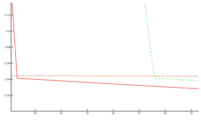
On the other hand the componentwise sparse control steers the system to consensus in time t = 22.3. Moreover the totally distributed control, acting on the whole group of 20 agents, steers the system in a larger time, t = 27.6. The time evolution of √V and of γ(X) is represented in Figure 4. In Figure 5 the detail of the moment in which the two systems enter the consensus region.

−1.5 −1 −0.5 0 0.5 1 1.5 −1.5 −1 −0.5 0 0.5 1 1.5

Figure 2: The initial configuration of Example 3.

0 10 20 30 40 50 60 70 80 90 100 0 0.2 0.4 0.6 0.8 1 1.2 1.4 1.6 1.8 2

Figure 3: The time evolution for t ∈ [0, 100] ofpV (t) (solid line) and of the quantity γ(X(t)) (dashed line). The system does not reach the consensus region.

0 5 10 15 20 25 30 0 0.2 0.4 0.6 0.8 1 1.2 1.4 1.6 1.8 2

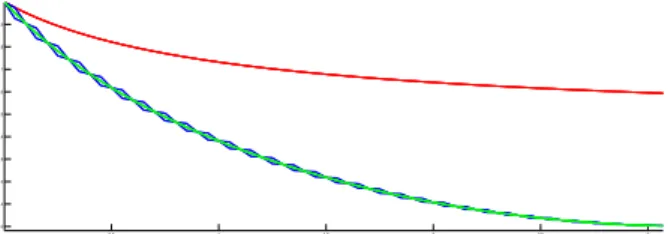
Figure 4: Comparison between the actions of the componentwise sparse control and the totally dis-tributed control. The time evolution for t ∈ [0, 30] ofpV (t) (solid line in the sparse case and dash-dot line in the distributed case) and of γ(X(t)) (dashed line in the sparse case and dotted line in the dis-tributed case).

23 24 25 26 27 28 29 0.102 0.104 0.106 0.108 0.11 0.112

Figure 5: Detail of the time evolution ofpV (t) and of γ(X(t)) under the action of the componentwise sparse control and the completely distributed control near the time in which the two systems enter the consensus region. The solid line represents the evolution ofpV (t) under the action of the componen-twise sparse control and the dash-dot line the evolution ofpV (t) under the action of the distributed control. The dashed line represents the evolution of γ(X(t)) under the action of the componentwise sparse control and the dotted line the evolution of γ(X(t)) under the action of the distributed control.

3.2 Complexity of consensus

The problem of determining minimal data rates for performing control tasks has been considered for more than twenty years. Performing control with limited data rates incorporates ideas from both control and information theory and it is an emerging area, see the survey Nair, Fagnani, Zampieri and Evans [44], and the references within the recent paper [15]. Similarly, in Information Based Complexity [46, 47], which is a branch of theoretical numerical analysis, one investigates which are the minimal amount of algebraic operations required by any algorithm in order perform accurate numerical approximations of functions, integrals, solutions of differential equations etc., given that the problem applies on a class of functions or on a class of solutions.

We would like to translate such concepts of universal complexity (universal because it refers to the best possible algorithm for the given problem over an entire class of functions) to our problem of optimizing the external intervention on the system in order to achieve consensus.

For that, and for any vector w ∈ Rd, let us denote supp(w) := {i ∈ {1, . . . , d} : ui 6= 0} and # supp(w) its cardinality. Hence, we define the minimal number of external interventions as the sum of the actually activated components of the control # supp(u(tℓ)) at each switching time tℓ, which a policy maker should provide by using any feedback control strategy u in order to steer the system to consensus at a given time T . Not being the switching times t0, t1, . . . , tℓ, . . . specified a priori, such a sum simply represents the amount of communication requested to the policy maker to activate and deactivate individual controls by informing the corresponding agents of the current mean consensus parameter ¯v of the group. (Notice that here, differently from, e.g., [44], we do not yet consider quantization of the information.)

More formally, given a suitable compact set K ⊂ (Rd)N _{× (R}d)N of initial conditions, the ℓN_{1 −} ℓd_{2-norm control bound M > 0, the set of corresponding admissible feedback controls U (M ) ⊂} B_ℓN

number as n := n(N, U (M ), K, T ) = inf u∈U (M) ( sup (x0,v0)∈K (_k−1 X ℓ=0

# supp(u(tℓ)) : (x(T ; u), v(T, u)) is in the consensus region ))

. Although it seems still quite difficult to give a general lower bound to the consensus numbers, Theorem 3 actually allows us to provide at least upper bounds: for T0 = T0(M, N, x0, v0_{, a(·)) =} 2N_M (p_{V (0) −} γ( ¯X)), and τ0 = τ0(M, N, x0, v0, a(·)) as in Theorem 3 and Remark 5, we have the following upper estimate

n(N, U (M ), K, T ) 6( ∞,sup_(x0,v0)∈KT0(M,N,x0,v0,a(·)) T < T0

inf_(x0,v0)∈Kτ0(M,N,x0,v0,a(·)), T > T0

. (28)

Depending on the particular choice of the rate of communication function a(·), such upper bounds can be actually computed, moreover, one can also quantify them over a class of communication functions a(·) in a bounded set A ⊂ L1(R+), simply by estimating the supremum.

The result of instantaneous optimality achieved in Proposition 3 suggests that the sampling strategy of Theorem 3 is likely to be close to optimality in the sense that the upper bounds (28) should be close to the actual consensus numbers. Clarifying this open issue will be the subject of further investigations which are beyond the scope of this paper.

4

Sparse Controllability Near the Consensus Manifold

In this section we address the problem of controllability near the consensus manifold. The stabilization results of Section 2 provide a constructive strategy to stabilize the multi-agent system (9): the system is first steered to the region of consensus, and then in free evolution reaches consensus in infinite time. Here we study the local controllability near consensus, and infer a global controllability result to consensus.

The following result states that, almost everywhere, local controllability near the consensus man-ifold is possible by acting on only one arbitrary component of a control, in other words whatever is the controlled agent it is possible to steer a group, sufficiently close to a consensus point, to any other desired close point. Recall that the consensus manifold is (Rd)N_{× Vf, where Vf} is defined by (5). Proposition 4. For every M > 0, for almost every ˜_{x ∈ (R}d)N and for every ˜_{v ∈ Vf}, for every time T > 0, there exists a neighborhood W of (˜x, ˜v) in (Rd)N _{× (R}d)N such that, for all points (x0, v0) and (x1, v1) of W , for every index i ∈ {1, . . . , N}, there exists a componentwise and time sparse control u satisfying the constraint (8), every component of which is zero except the ith

(that is, uj(t) = 0 for every j 6= i and every t ∈ [0, T ]), steering the control system (9) from (x0, v0) to (x1, v1) in time T . Proof. Without loss of generality we assume i = 1, that is we consider the system (9) with a control acting only on the dynamics of v1. Given (˜x, ˜v) ∈ (Rd)N × Vf we linearize the control system (9) at the consensus point (˜x, ˜v), and get d decoupled systems on RN _{× R}N

(

˙xk = vk

˙vk _{= −L}xv¯ k+ Bu , for every k = 1, . . . , d where

B =      1 0 .. . 0      .

To prove the local controllability result, we use the Kalman condition. It is sufficient to consider the decoupled control sub-systems corresponding to each value of k = 1, . . . , d. Moreover the equations for xk _{do not affect the Kalman condition, the x}k _{plays only the role of an integrator. Therefore we} reduce the investigation of the Kalman condition for a linear system on RN of the form ˙v = Av + Bu where A = −L¯x. Since A is a Laplacian matrix then there exists an orthogonal matrix P such that

D := P−1AP =       0 0 _{· · ·} 0 0 λ2 . .. ... .. . . .. ... 0 0 · · · 0 λN       .

Moreover since (1, . . . , 1) ∈ ker A, we can choose all the coordinates of the first column of P and thus the first line of P−1 = PT are equal to 1. We denote the first column of P−1 by

B1 =      1 α2 .. . αN      .

Notice that B1 = P−1B. Denoting the Kalman matrix of the couple (A, B) by K(A, B) = (B, AB, . . . , AN −1B)

one has

K(P−1AP, P−1B) = P−1K(A, B)

and hence it suffices to investigate the Kalman condition on the couple of matrices (D, B1). Now, there holds K(D, B1) =      1 0 0 _{· · ·} 0 α2 λ2α2 λ2₂α2 _{· · ·} λN −1₂ α2 .. . ... ... ... ... αN λNαN λ2_NαN · · · λN −1_N αN      .

This matrix is invertible if and only if all eigenvalues 0, λ2, . . . , λN are pairwise distinct, and all coefficients α2, . . . , αN are nonzero. It is clear that these conditions can be translated as algebraic conditions on the coefficients of the matrix A.

Hence, for almost every ˜_{x ∈ (R}d)N and for every ˜_{v ∈ Vf}, the Kalman condition holds at (˜x, ˜v). For such a point, this ensures that the linearized system at the equilibrium point (˜x, ˜v) is controllable (in any time T ). Now, using a classical implicit function argument applied to the end-point mapping (see e.g. [64]), we infer the desired local controllability property in a neighborhood of (˜x, ˜v). By construction, the controls are componentwise and time sparse. To prove the more precise statement of Remark 7, it suffices to invoke the chain of arguments developed in [59, Lemma 2.1] and [33, Section 2.1.3], combining classical needle-like variations with a conic implicit function theorem, leading to the fact that the controls realizing local controllability can be chosen as a perturbation of the zero control with a finite number of needle-like variations.

Remark 6. _{Actually the set of points x ∈ (R}d)N for which the condition is not satisfied can be expressed as an algebraic manifold in the variables a(kxi − xjk). For example, if x is such that all mutual distances kxi − xjk are equal, then it can be seen from the proof of this proposition that the Kalman condition does not hold, hence the linearized system around the corresponding consensus point is not controllable.

Remark 7. The controls realizing this local controllability can be even chosen to be piecewise con-stant, with a support union of a finite number of intervals.

As a consequence of this local controllability result, we infer that we can steer the system from any consensus point to almost any other one by acting only on one agent. This is a partial but global controllability result, whose proof follows the strategy developed in [16, 17] for controlling heat and wave equations on steady-states.

Theorem 4. For every (˜x0, ˜v0_{) ∈ (R}d)N_×Vf, for almost every (˜x1, ˜v1_{) ∈ (R}d)N_×Vf, for every δ > 0, and for every i = 1, . . . , N there exist T > 0 and a control u : [0, T ] → [0, δ]d steering the system from (¯x, ¯v) to (˜x, ˜v), with the property uj(t) = 0 for every j 6= i and every t ∈ [0, T ].

Proof. Since the manifold of consensus points (Rd)N_×Vf is connected, it follows that, for all consensus points (˜x0, ˜v0) and (˜x1, ˜v1), there exists a C1 path of consensus points (˜xτ, ˜vτ) joining (˜x0, ˜v0) and (˜x1, ˜v1), and parametrized by τ ∈ [0, 1]. Then the we apply iteratively the local controllability result of Proposition 4, on a series of neighborhoods covering this path of consensus points (his can be achieved by compactness). At the end, to reach exactly the final consensus point (˜x1, ˜v1), it is required that the linearized control system at (˜x1, ˜v1) be controllable, whence the “almost every” statement.

Note that on the one hand the control u can be of arbitrarily small amplitude, on the other hand the controllability time T can be large.

Now, it follows from the results of the previous section that we can steer any initial condition (x0, v0) ∈ (Rd)N × (Rd)N to the consensus region defined by (7), by means of a componentwise and time sparse control. Once the trajectory has entered this region, the system converges naturally (i.e., without any action: u = 0) to some point of the consensus manifold (Rd)N_{× Vf}, in infinite time. This means that, for some time large enough, the trajectory enters the neighborhood of controllability whose existence is claimed in Proposition 4, and hence can be steered to the consensus manifold within finite time. Theorem 4 ensures the existence of a control able move the system on the consensus manifold in order to reach almost any other desired consensus point. Hence we have obtained the following corollary.

Corollary 1. For every M > 0, for every initial condition (x0, v0) ∈ (Rd)N× (Rd)N, for almost every (x1, v1) ∈ (Rd)N × Vf, there exist T > 0 and a componentwise and time sparse control u : [0, T ] → (Rd₎N_{, satisfying (8), such that the corresponding solution starting at (x}

0, v0) arrives at the consensus point (x1, v1) within time T .

5

Sparse Optimal Control of the Cucker-Smale Model

In this section we investigate the sparsity properties of a finite time optimal control with respect to a cost functional involving the discrepancy of the state variables to consensus and a ℓN_{1 − ℓ}d₂-norm term of the control.

While the greedy strategies based on instantaneous feedback as presented in Section 2 model the perhaps more realistic situation where the policy maker is not allowed to make future predictions, the optimal control problem presented in this section actually describes a model where the policy maker is allowed to see how the dynamics can develop. Although the results of this section do not lead systematically to sparsity, what is interesting to note is that the lacunarity of sparsity of the optimal control is actually encoded in terms of the codimension of certain manifolds, which have actually null Lebesgue measure in the space of cotangent vectors.

We consider the optimal control problem of determining a trajectory solution of (9), starting at (x(0), v(0)) = (x0, v0) ∈ (Rd)N × (Rd)N, and minimizing a cost functional which is a combination of the distance from consensus with the ℓN

1 − ℓd2-norm of the control (as in [28, 29]), under the control constraint (8). More precisely, the cost functional considered here is, for a given γ > 0,

Z T 0 N X i=1 µ³ v_{i(t) −} 1 N N X j=1 vj(t) ´2 + γ N X i=1 kui(t)k ¶ dt. (29)

Using classical results in optimal control theory (see for instance [5, Theorem 5.2.1] or [10, 64]), this optimal control problem has a unique optimal solution (x(·), v(·)), associated with a control u on [0, T ], which is characterized as follows. According to the Pontryagin Minimum Principle (see [54]), there exist absolutely continuous functions p_{x(·) and pv(·) (called adjoint vectors), defined on [0, T ]} and taking their values in (Rd)N, satisfying the adjoint equations

             ˙pxi = 1 N N X j=1 a(kxj− xik) kxj− xik hxj− xi, vj − vii(pvj− pvi), ˙pvi = −pxi− 1 N X j6=i

a(kxj− xik)(pvj− pvi) − 2vi+

2 N N X j=1 vj, (30)

almost everywhere on [0, T ], and pxi(T ) = pvi(T ) = 0, for every i = 1, . . . , N . Moreover, for almost

every t ∈ [0, T ] the optimal control u(t) must minimize the quantity N X i=1 hpvi(t), wii + γ N X i=1 kwik, (31)

over all possible w = (w1, . . . , wN) ∈ (Rd)N satisfying PN_i=1kwik 6 M.

In analogy with the analysis in Section 2 we identify five regions O1, O2, O3, O4, O5 covering the (cotangent) space (Rd)N _{× (R}d)N _{× (R}d)N _{× (R}d)N:

O1 = {(x, v, px, p_{v) | kpv}ik < γ for every i ∈ {1, . . . , N}},

O2 = {(x, v, px, p_{v) | there exists a unique i ∈ {1, . . . , N} such that kpv}ik = γ and kpvjk < γ for every

j 6= i},

O3 = {(x, v, px, pv) | there exists a unique i ∈ {1, . . . , N} such that kpvik > γ and kpvik > kpvjk for

every j 6= i},

O4 = {(x, v, px, p_{v) | there exist k > 2 and i1}, . . . , ik ∈ {1, . . . , N} such that kpv_i1k = kpv_i2k = · · · = kpvikk > γ and kpvi1k > kpvjk for every j /∈ {i1, . . . , ik}},

O5 = {(x, v, px, p_{v) | there exist k > 2 and i1}, . . . , ik ∈ {1, . . . , N} such that kpv_i1k = kpv_i2k = · · · = kpv_ikk = γ and kpvjk < γ for every j /∈ {i1, . . . , ik}}.

The subsets O1and O3are open, the submanifold O2is closed (and of zero Lebesgue measure) and O1∪ O2∪ O3 is of full Lebesgue measure in (Rd)N_{× (R}d)N_{. Moreover if an extremal (x(·), v(·), px(·), pv(·))} solution of (9)-(30) is in O1∪O3 along an open interval of time then the control is uniquely determined from (31) and is componentwise sparse. Indeed, if there exists an interval I ⊂ [0, T ] such that (x(t), v(t), px(t), pv(t)) ∈ O1 for every t ∈ I, then (31) yields u(t) = 0 for almost every t ∈ I. If (x(t), v(t), px(t), pv(t)) ∈ O3 for every t ∈ I then (31) yields uj(t) = 0 for every j 6= i and ui(t) =