A Bootstrap Test for the Probability of Ruin in the Compound Poisson Risk Process

(1)

IN THE COMPOUND POISSON RISK PROCESS BY

BENJAMIN BAUMGARTNERAND RICCARDO GATTO

ABSTRACT

In this article we propose a bootstrap test for the probability of ruin in the compound Poisson risk process. We adopt the P-value approach, which leads to a more complete assessment of the underlying risk than the probability of ruin alone. We provide second-order accurate P-values for this testing problem and consider both parametric and nonparametric estimators of the individual claim amount distribution. Simulation studies show that the suggested boot-strap P-values are very accurate and outperform their analogues based on the asymptotic normal approximation.

KEYWORDS

Edgeworth expansion, exponential and log-normal claim amounts, normal approximation, P-value, pivotal quantity, resampling, second-order accuracy.

1. INTRODUCTION

The risk process is a stochastic model for the variations of an insurer’s surplus over time. More precisely, if we denote by r0 ≥ 0 the initial reserve, by c > 0 the constant premium rate and by {Zt}t ≥ 0 the compound Poisson process of the

aggregate claim amounts, then the classical risk process {Yt}t ≥ 0 is given by

r ct Z

t = 0+ - t

Y , (1)

for all t ≥ 0. Precisely, Zt = i=t0Xi N

/

for all t ≥ 0, where X₀def₌ 0, for convenience, X₁, X2, … > 0 are independent individual claim amounts with common distri-bution function F and independent of the Poisson process {Nt}t ≥ 0 as well.

Let us denote by l > 0 the intensity of the Poisson process and assume that m def₌ E[X_{1] ! ( 0, 3 ). We defi ne the relative security loading b through c =}

( 1 + b )lm. The quantity of interest in this article is the probability of ruin

within the infi nite time horizon, namely the probability that {Yt}t ≥ 0 ever falls

93216_Astin40_1_10.indd 241

93216_Astin40_1_10.indd 241 11-05-2010 09:40:3011-05-2010 09:40:30

use, available at https:/www.cambridge.org/core/terms. https://doi.org/10.2143/AST.40.1.2049227

(2)

below the zero level. It is a well-known risk measure for an insurance company. By defi ning the time of ruin as

if this infi mum exists,

= inf : T t 0 t<0 3 $ , , Y # * -otherwise,

the probability of ruin is usually expressed as c( r0 ) = P( T < 3). We will later use a functional notation for it, see (3) below. We assume c > lm, i.e. b > 0,

otherwise ruin occurs with probability one. Two general references are Gerber (1979) or Bowers et al. (1997, Chapter 13).

Let us denote by r the adjustment coeffi cient, i.e. the positive solution in v of

#

₀3evxdF( )x =1₊cv/ ,l and assume it exists. An analytical formula for the probability of ruin is given by

Y r ( r r -T r e < e 0 0 3 c = E ) T , 8 B (2)

see Bowers et al. (1997, p. 413). Formula (2) can be obtained in various ways: by martingale theoretic arguments, see Asmussen (2000, p. 24-25), by Lund-berg conjugation, see Asmussen (2000, p. 69-71), or by ad hoc argumentations, see Bowers et al. (1997, p. 426-427). With the exception of exponentially dis-tributed claim amounts, this formula is however not suitable for numerical evaluations. Various numerical methods for evaluating the probability of ruin have been proposed. Dufresne and Gerber (1989) propose a recursive algo-rithm based on a discretization and we will use this method in Section 3, see also the Appendix for a summary of it. Asmussen (1985) suggests the use of stochastic simulation based on importance sampling for computing the prob-ability of ruin with a bounded relative error. The saddlepoint approximation is a method of asymptotic analysis that allows to approximate certain complex integrals with a bounded relative error. It provides another effi cient way of computing the probability of ruin, see Barndorff-Nielsen and Schmidli (1995) and Gatto (2008). Another approach proposed by Asmussen and Rolski (1991) is to consider phase-type individual claim amount distributions. Phase-type distributions include fi nite mixtures of exponential and Gamma distributions, but do not include heavy-tailed distributions, like the log-normal. Nevertheless,

any distribution on ⺢+ can be approximated with arbitrary accuracy by a

phase-type distribution. A phase-type individual claim amount distribution leads to a computable formula for the probability of ruin. However, it should be mentioned that phase-type distributions can easily involve a large number of parameters. Estimating these parameters from observed individual claim amounts can be diffi cult.

In this article we consider a testing problem instead of the single evaluation of the probability of ruin. This allows to take into account the uncertainty of the data used to estimate the unknown model parameters. Furthermore, we

93216_Astin40_1_10.indd 242

93216_Astin40_1_10.indd 242 11-05-2010 09:40:3011-05-2010 09:40:30

(3)

suggest the P-value approach to this testing problem, which tells us how dis-tant the probability of ruin is from a specifi ed threshold c0, and we propose computing the P-value by the bootstrap. The bootstrap test relies on the asymptotic normality shown by Pitts (1994) and on the jackknife estimator of the variance of the bootstrap probability of ruin. From a practical point of view, the insurer can fi x a threshold value c0 ! ( 0,1 ) for the probability of ruin, above which the business is considered too risky. Because typical prob-abilities of ruin in both life and non-life sectors are below 1%, the values of the threshold c0 should also be taken around 1%. Alternatively, this threshold value could also be imposed by law. We can note, however, that there are pre-sumably insurance companies working under substantially higher probabilities of ruin than 1%. This is often a consequence of insuffi cient legal constraints, which give important freedom to the companies in building their reserves and thus in offering attractive premiums. The fact that some Swiss health insurance companies have gone to ruin in these recent years seems to confi rm this presumption.

More precisely, we propose a bootstrap P-value for the testing problem given by (5) below as a measure of risk. There are obviously alternative meas-ures of risk that are used by insurance companies. Though, the scope of this paper is not to review or to compare various measures of risk, but to propose a new testing problem approach together with an accurate computational method as an improvement to the simple evaluation of the probability of ruin, which is a classical and established risk measure in the actuarial literature.

The rest of this article is organized as follows. At the beginning of Section 2, we give a short review of applications and developments of the bootstrap within the actuarial risk theory. In Subsection 2.1 we provide a precise descrip-tion of the testing problem proposed, in Subsecdescrip-tion 2.2 we give a bootstrap P-value and we justify its asymptotic second-order accuracy. Some concluding remarks are given in Subsection 2.3. In Section 3 we show the numerical accuracy of the proposed P-value by an involved two-level simulation study, in which we consider the exponential and the log-normal claim amount distri-butions. We also compare our bootstrap P-value with the one obtained from the asymptotic normal approximation and show that the bootstrap P-value is substantially more accurate than the asymptotic normal one.

2. THEBOOTSTRAPTEST

The bootstrap goes back to Efron (1979) and some general references are Efron (1982), Hall (1992) and Davison and Hinkley (2003). Some important applications and theoretical developments of the bootstrap in the context of actuarial risk theory are the following. Embrechts and Mikosch (1991) pro-pose a bootstrap procedure for estimating the adjustment coeffi cient of a risk process under the assumption that the distribution of the number of summands is known, but the common distribution function F of the summands is unknown

93216_Astin40_1_10.indd 243

93216_Astin40_1_10.indd 243 11-05-2010 09:40:3011-05-2010 09:40:30

(4)

and estimated by a sample. The adjustment coeffi cient is a central quantity that allows to compute the probability of ruin or the Cramér-Lundberg approxima-tion to it and it is also a measure of risk itself. Their emphasis is on a theo-retical justifi cation of the strong consistency of the bootstrap estimator of the adjustment coeffi cient. Pitts et al. (1996) consider again the case where F is unknown. They propose bootstrap and jackknife confi dence bounds for the adjustment coeffi cient, which is re-expressed as a functional of F. Hipp (1989a) considers asymptotic normal and bootstrap confi dence intervals for the infi -nite horizon probability of ruin when F is unknown and a sample from it is available. Pitts (1994) proposes a bootstrap estimator of the distribution function of a random sum, under the assumption that the distribution of the number of summands is known, but the common distribution of the inde-pendent summands is unknown and estimated by a sample. The distribution function of the random sum is expressed as a functional of the unknown distribution function of the summands and it is shown that the bootstrap ver-sion of this functional is strongly consistent and asymptotically normal, under some continuity and differentiability assumptions on the functional. Bootstrap confi dence bands for the whole distribution function are also developed. These results are then applied to the infi nite horizon probability of ruin of the clas-sical risk process by using its well-known geometric sum representation, see Pitts (1994, Section 5.4). Politis (2003) considers the classical risk process in the case where both the individual claim amount distribution function F and the Poisson intensity l are unknown. He proves the strong consistency and the

asymptotic normality of the bootstrap estimator of the infi nite horizon prob-ability of ruin, under general conditions on F and using the functional approach. Loisel et al. (2008) suggest to re-express the fi nite horizon probability of ruin as a functional of the individual claim amount distribution function F and to use the quantiles of the bootstrap estimator of the fi nite horizon probability of ruin as a measure of risk. They also provide some formulae for the infl uence function ( which is a directional derivative at F ) of the fi nite horizon probability of ruin. From this infl uence function, they obtain the asymptotic variance of the bootstrap estimator of the fi nite horizon probability of ruin and they also show its asymptotic normality when the initial reserve is zero.

In Subsections 2.1 and 2.2 we suggest a testing problem for the probability of ruin in the infi nite time horizon when F is unknown, but a sample from it is available. We then provide a bootstrap P-value to this testing problem, which is asymptotically more accurate than the asymptotic normal P-value.

2.1. The testing problem

Let us assume that the probability of ruin can be expressed as the functional 3

( r0) : "[ F7 F( < )

c ;$ F 0, 1], P T , (3)

where F denotes the infi nite dimensional space of distribution functions on ⺢+ with fi nite expectation, which are the individual claim amount distribution

93216_Astin40_1_10.indd 244

93216_Astin40_1_10.indd 244 11-05-2010 09:40:3011-05-2010 09:40:30

(5)

functions, and where PF denotes the probability measure of the underlying fi

l-tered probability space that assigns distribution function F to the individual claim amounts. For notational convenience, the initial reserve will serve as a parameter to this functional so that, for any fi xed F ! F, c( F; r0 ) becomes a function of r0 ≥ 0. The functional (3) can be defi ned explicitly as

L p ;r _k ;r (F ) 1 (F ), k 0 0 0 c = - 3 = F*k

/

where pk = b ( 1 + b ) – ( k + 1 )

, FL* k denotes the k-th convolution power of FL, for k ! {0, 1, …}, m( F ) = 3xd ( )x 0 F

#

and ( ) F y 1 -L x ( ) _{( )} F F x 1 0 = _{m F} dy ;

#

7 A (4)

for all x ≥ 0. The functional representation (3) to the probability of ruin is the one adapted by Pitts (1994, p. 551). We consider F unknown and distinguish the following two situations. In the fi rst one, F belongs to a parametric class, which is a fi nite dimensional subset of F, with one or more unknown param-eters that need to be estimated by the observed claim amounts that occurred within the time interval [0, t], for some t ! ( 0, 3). In the second situation,

F ! F is fully unknown and estimated by the empirical distribution function of the observed claim amounts incurred during [0, t]. Note that the fi nite time interval [0, t] is only considered for the estimation of F and that we are still considering probabilities of ruin over the infi nite time horizon.

Our parameter of interest is c( F; r0 ), where r0 is a fi xed initial reserve, for which we suggest the testing problem specifi ed by the null and the alternative hypotheses ; ; r r : ( ) : ( ) . F F H H < 0 0 0 0 0 1 c c c c = , (5)

Undervaluing the probability of ruin in an insurance company could lead to inappropriate managerial decisions, for example to an excessive reduction of the capital, which can be dangerous for the company. With the null and alternative hypotheses formulated in (5), the risk of undervaluation of the probability of ruin is controlled by the error of the fi rst kind or the size of the test, which is chosen very small ( typically between 1% and 5% ). A P-value for this testing problem is given in Subsection 2.2 and approximated with the bootstrap principle. 2.2. The bootstrap P-value

As already mentioned, it is often preferable to consider the testing problem (5) instead of a single evaluation of the probability of ruin. In this testing problem,

93216_Astin40_1_10.indd 245

93216_Astin40_1_10.indd 245 11-05-2010 09:40:3011-05-2010 09:40:30

(6)

it is also more informative to quantify the closeness of the null model to the observed data instead of simply deciding between rejecting the null model or not. The P-value approach leads to this quantifi cation, as a large P-value refl ects high coherence of the null model with the data.

Suppose that exactly n claim amounts occur during the time interval [0, t], hence that Nt = n for some t ! ( 0, 3) and n ! {1, 2, …}. Denote by Fn(x ) =

{X x

1

i=11

n-

/

n _i# }, for all x > 0, the empirical distribution function of the claim amounts occurring during [0, t]. Consider the functionals

n

;r n ( r

(F 0) var F; 0)

s2 = F_ c i,

the variance being taken under PF and based on the Nt = n random claim

amounts that occur during [0, t], and

n n ( ( ; r r r ( ; ; ) ; ) ( ) F F R z F_n _F n F z 0 0 0 # s -c P c = , ) f p (6)

where F ! F and z ! ⺢. Denote by Fnobs the empirical distribution of n observed

claim amounts, i.e. a realization of Fn. Then

n n c ( ( R { ; r = n ; F F sup F ( ) } n F F n ₀ 0 0 F 0 0 s c c = -! :c obs obs P r r ; ) ; ) f p (7)

is a P-value for the testing problem (5). Unfortunately, computing the P-value (7) in general involves two major diffi culties: the fi rst one is the determination of the distribution of the studentized probability of ruin under all F ! F such that c( F; r0 ) = c0 and the second one is the evaluation of the supremum over this subset of F. The second diffi culty can be reduced by assuming a simple parametric model for the individual claim amounts, which would restrict the search for the supremum from over an infi nite dimensional to over a low dimensional space. Nevertheless, in some practical situations it is preferable to avoid this assumption.

As mentioned in the beginning of Section 2, the asymptotic normality of the probability of ruin is established by Pitts (1994, Theorem 5.2). Thus, a fi rst general solution to our problem is to rely on the asymptotic normal approxi-mation ( ; ) lim ( ; ) ( ), k z F R z F z n n 0 def F = _{" 3} =

for all z ! ⺢ and all F ! F, where F denotes the standard normal distribution function. The independence of the above limit from F is a consequence of the

93216_Astin40_1_10.indd 246

93216_Astin40_1_10.indd 246 11-05-2010 09:40:3111-05-2010 09:40:31

(7)

( asymptotic ) pivotality obtained by studentizing the estimator of the probability of ruin in (6). The asymptotic P-value

n n n n , A ( ( ( ( k n ; n , F F F F F n 0 0 0 0 0 0 0 s c c s c c F = obs - = -obs obs obs r r r r P ; ) ; ) ; ) ; ) f p f p (8)

for all F ! F, can be evaluated directly, but it is only fi rst-order accurate, in the sense that, for all F ! F,

, An Pn O(n 2 as n . 1 " 3 - = -P ), (9)

The asymptotic error in (9) follows from expansion (11) below. An asymptotic improvement to (9) can be obtained by applying the bootstrap principle as follows. Consider n n n n ( ( r ( r F ( F) P ; ) ; ) , F F F R z n z 0 0 0 n # c s = * -_* ; n c r ; ) f p (10)

for all z ! ⺢, where PFn is the conditional probability measure where the unknown F has been replaced by Fn ! F, given the claim amounts X1, …, Xn

during [0, t], and where Fn* denotes the empirical distribution function of a

random sample generated from Fn, given X1, …, Xn. From the asymptotic

nor-mality of the probability of ruin, we can assume that the expansion

- -( ; ) ( ; ) ( ; ) ( ), , R z F_n k z F₀ n 2 ₁ z F o n asn 1 2 1 " 3 = + k + (11) holds, thus n n - n -( ) ( ) ( ) ( ), . R_n k₀ n 2 ₁ o_P n asn 1 2 1 " 3 = + + ;F ;F ;F z z k z

Given two sequences of random variables {Un}n ≥ 0 and {Vn}n ≥ 0, the notation Un = oP( Vn ), as n " 3, means that Un /Vn "

P

0, as n " 3. Expansion (11) is in

fact an Edgeworth expansion combined with expansions of the fi rst cumulants of the studentized probability of ruin and k1( z; F ) is the product of a polyno-mial of degree two in z with the standard normal density at z, refer to Hall (1992, Section 2.3) for further explanations. Because k1( z; Fn ) – k1( z; F ) = oP( 1 ), as n " 3, and k0( z; F ) = F( z ) is in fact independent of F, we have

n -( ) ( ; ) ( ) , Rn R z Fn oP n 2 asn 1 " 3 - = , ;F z (12)

for all F ! F. Defi ning

93216_Astin40_1_10.indd 247

93216_Astin40_1_10.indd 247 11-05-2010 09:40:3111-05-2010 09:40:31

(8)

n n ( ( ; F F P_B, R_n n _n 0 0 0 c s = obs -obs n c , r r ; ) ; ) F f p (13)

approximation (12) yields, for all F ! F, -( ) , P_B, P_n o_P n 2 asn 1 " 3 - = , n

whose comparison with (9) shows that the bootstrap P-value PB, n is asymp-totically more accurate than the asymptotic P-value PA, n. PB, n is second-order accurate, whereas PA, n is fi rst-order accurate.

In the remaining part of this section we give some remarks. The P-values

Pn, PA, n and PB, n are all based on n observed claim amounts, i.e. n realizations

from F. If we replace these observed claim amounts by their random counter-part, we obtain the random versions of these P-values, denoted by Pn, PA, n and

PB, n respectively. It can be shown that

n

( u u

F # #

P P ) , (14)

for all u ! [0, 1] and all F ! F such that c( F; r0 ) = c0. This allows for the following error rate interpretation: if we decide to reject H0 whenever a P-value is smaller than or equal to Pn, then (14) shows that the probability of a false

rejection is smaller than or equal to Pn. For a general reference about P-values,

see Casella and Berger (2002, Section 8.3.4).

If we had a simple null hypothesis, the supremum in the defi nition of Pn in

(7) would be irrelevant and, as a consequence, the weak inequality outside the probability in (14) would become an equality. In this case, (14) would tell that the P-value is uniformly distributed. But because neither PA, n nor PB, n involve the supremum, it follows that both PA, n and PB, n are asymptotically uniformly distributed. The uniformity of both PA, n and PB, n will be checked in the simulation study of Section 3.

As already mentioned, computing the probability of ruin is generally not a simple problem. We suggest using a numerical approximation introduced by Dufresne and Gerber (1989), which yields upper and lower bounds with arbi-trary precision. It is briefl y outlined in the Appendix.

For the estimation of the standard error of the estimator of the probability of ruin we use the jackknife. The jackknife is a useful nonparametric technique that allows to estimate various types of quantities and that shares some simi-larities with the bootstrap, see Quenouille (1949), Tukey (1958), Efron (1979) and Efron (1982). Typical applications are for bias and variance estimation. In our situation, the jackknife estimator of the standard error is given by

, 1 , 1 i -n 1 n- n j 1 1 ( r r r n F; ) n F ; F ; , n n 1 n 1 n 0 - 0 0 s - c - c j i= = 2 ` ` f j

/

jp

/

(15) 93216_Astin40_1_10.indd 248 93216_Astin40_1_10.indd 248 11-05-2010 09:40:3111-05-2010 09:40:31

(9)

where, for i ! {1, …, n}, Fn – 1, i is the i-th “leave-one-out” version of Fn, i.e., the

empirical distribution function based on the sample X1, …, Xi – 1, Xi + 1, …, Xn.

2.3. Remarks

In principle, the results derived in this article can be extended to the prob-ability of ruin within a fi nite time horizon. In this case, we should fi rst note that the proof of the asymptotic normality of the probability of ruin given by Pitts (1994, Theorem 5.2) is valid in the infi nite horizon only. Loisel et al. (2008) prove the asymptotic normality of the fi nite horizon probability of ruin only in the case where the initial reserve is zero. However, numerical simula-tions in Loisel et al. (2008, Section 7.1) seem to confi rm that the asymptotic normality holds for positive initial reserves as well, and this could be suffi cient for extending our bootstrap test. Note also that the algorithm used in Section 3 for computing the probability of ruin and summarized in the Appendix is no longer valid for the fi nite horizon situation.

Both remarks above remain valid if we were interested in probabilities of ruin, within either the infi nite or the fi nite time horizons, under a general renewal process instead of the Poisson process: we would not have asymptotic normality proofs and we would need an alternative algorithm for the compu-tation of the probabilities of ruin.

3. SIMULATIONRESULTS

In this section we present two simulation studies that compare the accuracy of the bootstrap with the asymptotic P-values presented in Subsection 2.2. The programs of the computations made in this section are written in the language R, see R Development Core Team (2008). They can be found in the software section at

http://www.stat.unibe.ch/content/research/publications.

For the fi rst simulation study we consider the nonparametric bootstrap approach. Each sample of claim amounts is generated from an exponential distribution and the bootstrap P-value is computed by resampling from the generated sample. For the second simulation study, we consider the parametric bootstrap approach. Each sample of claim amounts is generated from a log-normal distribution and the bootstrap P-value is computed by generating samples from the log-normal distribution with parameters estimated from the generated sample. The results of both simulations are placed side-by-side in the graphs of Figures 1-4. The left graphs refer to the nonparametric approach and the right ones refer to the parametric approach. In both situations we have considered a two-level simulation design in which we fi rst generate 1000 sam-ples and then, for each sample, we generate 1000 bootstrap samsam-ples. Following

93216_Astin40_1_10.indd 249

93216_Astin40_1_10.indd 249 11-05-2010 09:40:3111-05-2010 09:40:31

(10)

Hipp (1989a), we assume lm ( the mean payment per unit of time ) known. This

assumption avoids diffi culties arising whenever the condition c > lm is violated

by l and m replaced by estimated values. Since the parameters l, m and c

appear in the computation of the probability of ruin only through lm / c =

( 1 + b )–1 = c( F; 0 ), this assumption reduces to b known. For both simulations

studies we take b = 0.2 and lm = 10 and thus c( F; 0 ) = 10/12. Note that the

knowledge of l is not necessary in these simulation studies. Practically, there

is no need to simulate the Poisson process. We simply generate n claims that are supposed to belong to the time interval [0, t], for some t ! ( 0,3).

In the fi rst simulation study we generate bootstrap P-values when the indi-vidual claim amount distribution F is estimated by the empirical distribution of the individual claim amounts. We simulate 1000 samples of n = 250 indi-vidual claim amounts from the exponential distribution with mean 10. The probability of ruin is computed with the recursive method given in the Appen-dix, where the distribution function FL defi ned in (4) is replaced by the

estima-tor given in (18) in the Appendix.

In the second simulation study, bootstrap P-values are based on the para-metric estimation of the individual claim amount distribution. We generate 1000 samples of n = 100 individual claim amounts from the log-normal distri-bution F, where the logarithmic random variable has mean 2 and variance 0.6. Lower and upper bounds to the probability of ruin are again computed with the recursive algorithm of the Appendix, where the distribution FL defi ned in

(4) is replaced by a parametric estimator of it, by estimating the parameters of

F and by numerical integration. In both simulation studies the probabilities of

ruin are obtained by taking the average of the upper and the lower bounds defi ned in (17), using discretization steps of 1 for the estimators of the prob-ability of ruin and of 4 for the estimator of the standard error given in (15).

FIGURE 1: Kernel estimators of the density of the studentized probability of ruin based on bootstrap replications ( solid lines ) and on simulations ( dashed lines ) with the standard normal density ( dotted lines )

for exponential ( left ) and log-normal claims ( right ).

93216_Astin40_1_10.indd 250

93216_Astin40_1_10.indd 250 11-05-2010 09:40:3111-05-2010 09:40:31

(11)

Figure 1 compares the standard normal density with the kernel density estimators of the studentized probabilities of ruin obtained by 1000 simulations and by 1000 ≈ 1000 bootstrap replications. For both the simulated probabilities of ruin and the bootstrap probabilities of ruin we use the kernel density estima-tor with Gaussian kernels with bandwidths 0.25 and 0.1, respectively. Clearly, the density of the studentized probabilities of ruin is better approximated by the bootstrap densities than by the asymptotic normal densities, which are particularly misleading in the left tails. Figure 2 compares the distribution functions of the bootstrap and asymptotic P-values with the uniform distribution

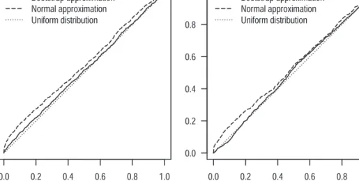
FIGURE 2: Empirical distribution functions of the bootstrap ( solid lines ) and asymptotic normal ( dashed lines ) P-values with the uniform distribution function on [0, 1] ( dotted lines ) for exponential ( left )

and log-normal claims ( right ).

FIGURE 3: Estimated densities of the bootstrap ( solid lines ) and normal ( dashed lines ) P-values with the uniform density on [0, 1] ( dotted lines ) for exponential ( left ) and log-normal claims ( right ).

93216_Astin40_1_10.indd 251

93216_Astin40_1_10.indd 251 11-05-2010 09:40:3211-05-2010 09:40:32

(12)

function on [0, 1]. In both graphs we can see that the bootstrap P-values are closer to uniformity than the asymptotic ones. Thus, bootstrap P-values allow for accurate error rate interpretations, as explained at the end of Subsection 2.2. Asymptotic normal P-values are not close to uniformity and (14) is especially violated for small values, which are the most important ones for the error rate interpretation. Figure 3 shows the densities corresponding to Figure 2. Because the support of the distribution of P-values is bounded, the density estimators of the P-values in Figure 3 use a Gaussian copula-based method with under-lying correlation 0.9 instead of the kernel density estimator, see Jones and Henderson (2007) for details. Figure 4 shows how the proportions of P-values smaller than or equal to 0.05 ( indicated by the horizontal lines ) behave as functions of c₀ with all other parameters left unchanged, for both simulation studies. Because the point c₀ = c( F; r₀ ) ( indicated by the vertical lines ) cor-responds to the case under which the simulation is performed, it follows from (14) that the proportion at this point should be lower than or equal to 0.05, which is the level of the test that rejects H₀ for P-values smaller than or equal to 0.05. In both simulation studies, this proportion at this point is close to 0.05 with the bootstrap. The values corresponding to the asymptotic normal approximations exceed the level 0.05 signifi cantly.

ACKNOWLEDGEMENTS

The authors thank the editor-in-chief, two anonymous referees for their thoughtful comments and the Swiss National Science Foundation for its fi nan-cial support.

FIGURE 4: Proportion of bootstrap ( solid lines ) and normal ( dashed lines ) P-values smaller than or equal to 0.05 as a function of c0. The horizontal lines indicate the signifi cance level, the vertical lines indicate

c( F; r0 ) for exponential ( left ) and log-normal claims ( right ).

93216_Astin40_1_10.indd 252

93216_Astin40_1_10.indd 252 11-05-2010 09:40:3311-05-2010 09:40:33

(13)

APPENDIX

A RECURSIVE METHOD FOR COMPUTING THE PROBABILITY OF RUIN

In this appendix we summarize an algorithm proposed by Dufresne and Ger-ber (1989) for computing the probability of ruin within the infi nite horizon. Let us defi ne the aggregate loss process {St}t ≥ 0 = {Zt – ct}t ≥ 0 and let L1, L2, … denote the increments of its running maximum {max0 ≤ u ≤ t Su}t ≥ 0, recursively

defi ned by i=0 0 L and L_k S_inf_{_t _{0 :}_S _L L_i i k 0 0 1 > t i = = $ = -k-1 - , }

/

for k ! {1, 2, …}. It can be shown that the maximal aggregate loss S def₌ maxt ≥ 0

{St} = L1 + … + LN, where P( N = n ) = p( 1 – p )n, for all n ! {0, 1, …}, where p = 1 – c(F; 0 ), and L1, …, LN are independent with the distribution function FL(F; x ), for all x ≥ 0, defi ned by (4). The method presented here is essentially

based on a discretization of (4) and it leads to upper and lower bounds to

c(F; r0 ), with both bounds converging to c(F; r0 ) with decreasing discretiza-tion steps ( denoted j below ).

We can compute a lower and an upper bound for the maximal aggregate loss S by discretizing its summands L1, …, LN on a mesh of width j > 0 as

follows,

S(L) = j j₈ -1L₁_B+g+j j₈ -1L_N_B and S(U) = j j_` -1L₁_j+g+j j_` -1L_N_j_,

where ⎣x⎦ = max{k ! ⺪ : k ≤ x} and ⎡x⎤ = min{k ! ⺪ : k ≥ x}, for all x ! ⺢. From c( F; r0 ) = P( S > r0 ) and S ( L ) ≤ S ≤ S ( U ) it follows that

; r 1-P(S(L)<r₀) # c(F ₀) #1-P(S(U)#r₀) . (16) Let us defi ne P ( ; ( 1)) ( ; ), h_k( )L = j j_-₁L₁ jk = _L F j k+ _L F jk F F = -a 8 B k for k ! {0, 1, …}, and 1) 1 P ( ; ) ( ; (F ) h( )_kU = j _- L₁ j = _L F jk - _L j -F , k F j = k a ` j k

for k ! {1, 2, …}. Defi ne also, for i ! {0, 1, …},

i

i P(S i and f P(S i ) .

f( )L = (L)= j) ( )U = (U)= j

93216_Astin40_1_10.indd 253

93216_Astin40_1_10.indd 253 11-05-2010 09:40:3311-05-2010 09:40:33

(14)

From Dufresne and Gerber (1989, Section 2.4), the bounds of (16) can be obtained using the recursive formulae

k -i i i i-k 1 ( ; 0) ( ; ) , ( ; 0) f F h F h f f F h f 0 k k i k k i 1 1 0 c c c = -= = = ( ) ( ) ( ) L L U , U U ( ) ( ) ( ) ( ) L L

/

for i ! {1, 2, …}, with the initial values

( ; ) ( ; ) , 1 ( ; 0) . f F h F f F 1 0 1 0 0 0 0 c c c = = -( )L U ( ) ( ) L

Note that c( F; 0 ) = lm/c depends on F through its mean only. Precisely, using

(16), these bounds are given by

i i 1 1 ; r 1 f (F ) 1 f . 0 i i r r 0 0 1 0 0 # # c - -j- - j -= = U ( )L ( ) 8 B ` j

/

(17)

In the fi rst example of Section 3, F is unknown and estimated by the empirical distribution function Fn of the claim amounts. In this case we estimate FL by

n n n X ( ( ( ( 1 1 x x ; ) ) 1 ) , ( , 1 F min x n y X x X 1 1 1 _< L n i i n i i i i 0 0 ₁ m m = -= = = = = F F F n n ) F y y y d d ) 7 A #

-/

/

#

(18)

where n is the number of claims observed during [0, t].

REFERENCES

ASMUSSEN, S. (1985) Conjugate processes and the simulation of ruin problems, Stochastic Processes

and their Applications, 20, 213-229.

ASMUSSEN, S. (2000) Ruin Probabilities, vol. 2 of Advanced Series on Statistical Science and Applied Probability, World Scientifi c, Singapore.

93216_Astin40_1_10.indd 254

93216_Astin40_1_10.indd 254 11-05-2010 09:40:3311-05-2010 09:40:33

(15)

ASMUSSEN, S. and ROLSKI, T. (1991) Computational methods in risk theory: A matrix-algorithmic approach, Insurance: Mathematics and Economics, 10, 259-274.

BARNDORFF-NIELSEN, O.E. and SCHMIDLI, H.U. (1995) Saddlepoint approximations for the prob-ability of ruin in fi nite time, Scandinavian Actuarial Journal, 2, 169-186.

BOWERS, N., GERBER, H.U., HICKMANN, J., JONES, D. and NESBITT, C. (1997) Actuarial

Math-ematics, The Society of Actuaries, Schaumburg, Illinois, second edn.

CASELLA, G. and BERGER, R.L. (2002) Statistical Inference, Duxbury Advanced Series in Statis-tics and Decision Sciences, Duxbury Press, Pacifi ce Grove, California, second edn.

DAVISON, A.C. and HINKLEY, D.V. (2003) Bootstrap Methods and their Applications, no. 1 in Cambridge Series in Statistical and Probabilistic Mathematics, Cambridge University Press, Cambridge, reprinted and corrected edn.

DUFRESNE, F. and GERBER, H.U. (1989) Three methods to calculate the probability of ruin,

ASTIN Bulletin, 19, 71-90.

EFRON, B. (1979) Bootstrap methods: Another look at the jackknife, The Annals of Statistics, 7, 1-26.

EFRON, B. (1982) The Jackknife, the Bootstrap and Other Resampling Plans, no. 38 in CBMS-NSF Regional Conference Series in Applied Mathematics, Society for Industrial and Applied Math-ematics (SIAM), Philadelphia.

EMBRECHTS, P. and MIKOSCH, T. (1991) A bootstrap procedure for estimating the adjustment coeffi cient, Insurance: Mathematics and Economics, 10, 181-190.

GATTO, R. (2008) A saddlepoint approximation to the probability of ruin in the compound Pois-son process with diffusion, Statistics and Probability Letters, 78, 1948-1954.

GERBER, H.U. (1979) An Introduction to Mathematical Risk Theory, no. 8 in Huebner Foundation Monograph Series, S. S. Huebner Foundation for Insurance Education, Philadelphia. HALL, P. (1992) The Bootstrap and Edgeworth Expansion, Springer Series in Statistics,

Springer-Verlag, New York.

HIPP, C. (1989a) Estimators and bootstrap confi dence intervals for ruin probabilities, ASTIN Bul letin, 19, 57-70.

JONES, M.C. and HENDERSON, D.A. (2007) Kernel-type density estimation on the unit interval, Biometrika, 94, 977-984.

LOISEL, S., MAZZA, C. and RULLIÈRE, D. (2008) Robustness analysis and convergence of empirical fi nite-time ruin probabilities and estimation risk solvency margin, Insurance: Mathematics and

Economics, 42, 746-762.

PITTS, S.M. (1994) Non-parametric estimation of compound distributions with applications in insurance, Annals of the Institute of Statistical Mathematics, 46, 537-555.

PITTS, S.M., GRÜBEL, R. and EMBRECHTS, P. (1996) Confi dence bounds for the adjustment coef-fi cient, Advances in Applied Probability, 28, 802-827.

POLITIS, K. (2003) Semiparametric estimation for non-ruin probabilities, Scandinavian Actuarial

Journal, 1, 75-96.

QUENOUILLE, M.H. (1949) Approximate tests of correlation in time-series, Journal of the Royal

Statistical Society. Series B (Methodological), 11, 68-84.

R DEVELOPMENT CORE TEAM (2008) R: A Language and Environment for Statistical Computing, R Foundation for Statistical Computing, Vienna, Austria.

TUKEY, J.W. (1958) Bias and confi dence in not quite large samples (abstract), The Annals of

Mathematical Statistics, 29, 614.

BENJAMIN BAUMGARTNER and RICCARDO GATTO

Institute of Mathematical Statistics and Actuarial Science University of Bern Alpeneggstrasse 22 3012 Bern Switzerland E-mail: baumgartner@stat.unibe.ch E-mail: gatto@stat.unibe.ch 93216_Astin40_1_10.indd 255 93216_Astin40_1_10.indd 255 11-05-2010 09:40:3311-05-2010 09:40:33