HAL Id: hal-02790268
https://hal.inrae.fr/hal-02790268
Submitted on 5 Jun 2020
HAL is a multi-disciplinary open access archive for the deposit and dissemination of sci-entific research documents, whether they are pub-lished or not. The documents may come from teaching and research institutions in France or abroad, or from public or private research centers.
L’archive ouverte pluridisciplinaire HAL, est destinée au dépôt et à la diffusion de documents scientifiques de niveau recherche, publiés ou non, émanant des établissements d’enseignement et de recherche français ou étrangers, des laboratoires publics ou privés.
. Ku, . Irta, . Inra
To cite this version:
. Ku, . Irta, . Inra. Detailed specification for the calculation “engine” to be used in the DSS in Task 4.1. [Contract] D3.6, 2019. �hal-02790268�
Page 1/38
FEED-A-GENE
Adapting the feed, the animal and the feeding techniques to
improve the efficiency and sustainability of monogastric livestock
production systems
Deliverable D3.6
Detailed specification for the
calculation “engine” to be used in the
DSS in Task 4.1
Due date of deliverable: M48
Actual submission date: M48
Start date of the project: March 1
st, 2015
Duration: 60 months
Organisation name of lead contractor: KU
Revision: V1
Dissemination level
Public – PU
X
Confidential, only for members of the consortium (including Commission
Services) – CO
Page 2/38
Table of contents
1.
Summary ... 3
2.
Introduction ... 5
3.
Results ... 6
3.1.
Post-digestive model for pigs and broilers ... 6
3.2.
InraPorc model with an optimization module ... 12
3.3.
Feed intake module ... 13
3.4.
Layer model ... 17
4.
Conclusions ... 21
References ... 21
Page 3/38
1. Summary
Objectives:
The objective of the deliverable is to indicate how (elements of) the conceptual models that have been developed in WP3 can be used in the Decision Support Systems (DSS) developed in Task 4.1 for pigs and poultry.
Rationale:
A first version of an animal model to be used for the development of a DSS in Task 4.1 was provided as deliverable D3.1. This model was a modified version of the InraPorc model (for growing pigs) and addressed aspects of phosphorus and calcium metabolism. Elements of this deliverable have been used in Task 4.1 to develop decision support tools for the real-time determination of animal nutritional requirements (see deliverable D4.1). A real-real-time model was developed to calculate the appropriate feed and nutrient supply for an individual animal for the next day or period. This real-time model is based on the predicted feed intake and body weight gain from which the nutrient requirements (e.g., lysine) are determined. The modelling approaches of WP4 and WP3 are fundamentally different: WP4 uses real-time modelling using predictions of feed intake and body weight gain, while WP3 worked on modelling “once we have the data” and by “looking back”. Despite these differences, a number of issues and recommendations resulting from WP3 can be used in the real-time modelling of nutritional requirements.
WP3 aimed to develop mathematical models with different approaches including mechanistic dynamic models to simulate nutrient digestion (Task 3.1) and the post-digestive metabolism of nutrients in monogastric animals (Task 3.2). At this stage, the complete digestion model (deliverable D3.2) is probably not suited to be integrated in a decision support system for precision feeding. However, it has been generic in design for both pigs and poultry and the (simulated) effects of body weight and diet composition on digestibility can be used to construct empirical equations that can adjust (constant) table values of nutrient digestibility that are currently used in models and decision support systems.
This concept proposed in deliverable D3.1 has been developed further to address the effect of different environmental and nutritional aspects on feed intake and predictions of the fatty acid profile in different body components. Also, deliverable D3.1 did not include models for broilers and laying hens, and these aspects are addressed in the current deliverable.
Adaptations to the post-digestive metabolic model to including phosphorus (P) metabolism and adaptations to the feed intake module: The P-module represent phosphorus metabolism and predicts the effect of dietary digestible P supply on P retention and urinary P excretion. The model is integrated in InraPorc and simulates the regulatory mechanism of P supply such as that an insufficient P supply P limits growth and reduces the appetite of the animal. Also, in the original approach, daily feed intake is a phenotypic trait and driven by body weight, but it does not take explicitly into account that dietary and environmental factors can limit the actual feed intake. The updated feed intake module quantifies the effect of specific environmental effects of feed intake (e.g., ambient temperature, stocking density). Feed intake is very variable on a day-to-day basis (see deliverable D4.5), and we suggest that cumulative feed intake could provide a better basis for feed intake predictions. Cumulative
Page 4/38
feed intake represents a trajectory that the animal may seek to achieve. Rather than attempting to predict what an animal is going to eat tomorrow, it may be better to forecast feed intake for a longer time window, in which cumulative feed intake could be used as a target. The methodologies developed in Task 3.4 and reported in deliverable D3.5 can be used to construct confidence intervals for the predictions of feed intake and body weight gain. This can be used to determine the period for which reasonable predictions for body weight and (cumulative) feed intake can be made, which would also results in reasonable predictions of nutrient requirements in a decision support tool for precision feeding.
A broiler growth and laying hen model based on InraPorc: the InraPorc model predicting post-digestive nutrient utilization for growing pigs was adapted to broilers. Without major changes to the core structure of the model, species-specific parameters and equations were identified. The original pig model uses a generic approach to nutrient partitioning, and the adapted model was able to represent the similar, underlying mechanisms of nutrient partitioning for broilers. The same model core was also used for layers assuming that a laying hen is more mature than a broiler (i.e., with a lower body protein deposition) and has a priority to produce eggs. The model predicts the effect of the digestible nutrient supply, including energy, amino acids, Ca and P, on egg production.
The above-mentioned models are ready to be included in a DSS for precision livestock farming in different ways: i) the model-generated outputs can be compared with real-time collected data, and ii) the real-time daily or, preferable, the cumulative feed intake can be used as input in the simulation model to predict the performance for the next day(s). A difference between the simulation (expected trajectory) and real-time measurements can be used as inputs to an early warning system that can be used to identify technological or health problems. The concept of the robustness module (task 3.3 and deliverable D3.4) can also be considered for the DSS developed in task 4.1.
Teams involved: - KU, IRTA, INRA
- contact person on request of the source code: Veronika Halas, [email protected]
Species and production systems considered:
The models are developed for growing and fattening pigs, broilers, and layers irrespective of the geographical region and applies to all genotypes in different environmental conditions.
Page 5/38
2. Introduction
The efficiency of resource use and the efficiency of animal production can be improved by strict planning and control. In livestock production, modelling has served as an excellent tool to help the understanding and to predict the animal’s response to different farm conditions. Models are useful in planning, but also in controlling livestock production. Precision farming adopts real-time monitoring systems collecting serial data about individual animals or groups of animals. However, without a well-defined goal-oriented data process, data by itself are not useful. Available and newly recorded data can be converted to valuable information for management purposes through models applied in farming systems. Nowadays, models are more and more sophisticated to predict animal performance under different environmental and management conditions. Therefore, modelling is a key tool to improve the efficiency and sustainability of livestock production systems.
In animal nutrition, it is important to assess how the animal responds to the supply of nutrients, so that practical feeding decisions can be made. A properly calibrated growth model predicts in a dynamic way the performance of an individual or a group of animals by simulating changes in daily gain, feed conversion ratio, and the composition of the body in relation to different inputs. Growth models can therefore be used effectively to identify an appropriate strategy for grower–finisher pig, broiler, or layer farms by evaluating different management and feeding strategies and comparing the predicted outcomes. The optimal feeding strategy may depend on local market conditions (e.g., target live weight or carcass weight, carcass quality, preferred egg size), farm rotation system, and feed and labour costs. Based on input and output data, economic analyses of alternative feeding strategies can be assessed, which are essential in decision-making.
The aim of the modelling work in WP3 has been to develop a generic modelling platform to predict nutrient utilisation in pigs and poultry, while accounting for differences that exist among livestock species and production conditions. By transforming the concepts and knowledge into mathematical equations and integrating these into computer programs using simulation-modelling techniques and end-user tools, the information can be readily applied in commercial production systems. The conceptual models representing the feed-use mechanisms are now ready for further application. In WP3 of the Feed-a-Gene project, different approaches were used including a mechanistic dynamic approach to represent and simulate nutrient digestion (task 3.1) and the post-digestive metabolism of nutrients in monogastric animals (task 3.2).
Nutritional models typically rely on (static) table values for the nutritional value of feed ingredients. Although it is acknowledged that digestion has a major impact on nutrient utilization, remarkable little attention has been paid to understand, in a quantitative way, the digestion process. In task 3.1, we worked on a mechanistic description of the digestive process in pigs and poultry. Although it is not yet feasible, at this stage, to use such an approach in precision livestock feeding, the effect of body weight (and to some extent of diet composition) on digestibility has been quantified. This type of information could be included in the DSS of precision livestock farming systems to modulate table values of digestibility according to body weight (or diet composition, such as fibre content). The description of the digestion module is given in Deliverable D3.2.
Page 6/38
Models representing and predicting the post-digestive nutrient utilization (task 3.2) consist of different modules. The InraPorc model, representing the energy and amino acid metabolism of growing and fattening pigs, was developed further by integrating modules that simulate phosphorus metabolism and fatty acid partitioning. Also, a module to estimate the daily feed intake more accurately was developed. Based on the concepts of the InraPorc model, models for broiler growth and egg production of layers have been developed. To our knowledge, there are no models (publicly) available for broiler growth and egg production of layers. Except for the fatty acid module, all the modules of the pig model have been adapted for broilers.
In WP3 we worked in different programming environments like Excel, MATLAB and R. Excel sheets have been translated to MATLAB. These tools are free (R) or can be read and understood easily (MATLAB). They can be modified if necessary and be translated in dedicated modules of PLF systems. The code of the post-digestive pig model was reported in deliverable D3.1. The revised P-module and the new modules for feed intake and fatty acids are given in Annex 1.
3. Results
To formulate the diet, the anticipated feed intake for the next day needs to be predicted. InraPorc provides different options to represent the daily feed or energy intake like a linear, quadratic, and exponential function of body weight. Additionally, a more sophisticated function is also included to calculate the feed intake. This function is based on the premise that animals eat according to their energy requirement, thus there is a certain pattern during the lifetime and the energy intake can be expressed in times of maintenance energy needs. The feed intake module developed in WP3 accounts that factors other than body weight affect feed intake of the animal. The capacity of gastro-intestinal tract, the environmental temperature, stocking density and the P-supply relative to the requirements are considered as key modulating factors.
The deliverable D3.3 “A simulation model to predict the post-digestion nutrient use in monogastric animals” presents a detailed description of the InraPorc model, the feed intake module, and the P-module. Here we summarize the concepts and key equations of the models.
3.1. Post-digestive model for pigs and broilers
The post-digestive model simulates the partitioning of digestible nutrients (i.e., amino acids, fatty acids, starch, sugars, volatile fatty acid, Ca and P) and the conversion through intermediary metabolism to predict the net protein and lipid gain, the distribution of fatty acids in the body, phosphorus retention and animal performance according to its genetic potential. The time scale of the model is 1 day. The inputs of the model are digestible nutrients (i.e., amino acids (AA), fatty acids (FA), starch and sugars (ST+SU), volatile fatty acids (VFA) calcium (Ca), and phosphorus (P) and characteristics of the genotype. For growing and fattening animals, the animal is characterized by traits describing the feed intake capacity of the animal and traits related to the potential protein deposition and energy utilization. Feed intake capacity (expressed on a feed or energy basis) can de described by different types of equations, all of which can be expressed as the anticipated feed intake at two different body weights (i.e., at 50 and 100 kg for pigs or 1 and 2 kg for broilers). Traits related to potential
Page 7/38
protein deposition include the initial body (and protein) weight, the average protein deposition during the growing-finishing phase (meanPD), and a shape parameter of the protein deposition curve indicating if protein deposition occurs early or later (precocity). An additional parameter can be used to define how the protein deposition responds to a change in energy intake. Furthermore, the digestible nutrient content of the mixed feed is a model input. Either nutrient content and digestibility coefficients, or digestible nutrient content of the mixed feed have to be provided, which can user-defined or obtained from an internal AFZ database. Alternatively, the data on the supply of digestible nutrients can be obtained from the digestive model developed in task 3.1 (deliverable D3.2).
Outputs of the post-digestive model are body protein and lipid mass, fatty acid composition of the whole body and of backfat, body weight, feed conversion ratio, urinary N and P excretion, and retained P. Further outputs of the model used by task 4.1 are the expected feed intake, expected daily gain, from which the nutrient requirements for protein and phosphorus retention are determined.
The InraPorc model for growing and fattening pigs has not been modified. The model has been translated in Matlab format for use in task 4.1 (deliverable D3.3) and details of the model have been documented elsewhere (van Milgen et al., 2008). New modules developed in the Feed-a-Gene project have not yet been published. The concepts of these modules have been described in Deliverable D3.3 and are briefly summarized here.
The fatty acid module predicts the fatty acid composition of the body and backfat in fattening pigs. The model equations estimate metabolic (i.e., dietary and de novo synthesized fatty acids) and spatial (allometry) distribution of fatty acid deposition. It is hypothesized that differences in fatty acid composition between tissues can be explained by differences in tissue development combined with differences in the origin of fatty acids. The phosphorus module simulates the utilization of dietary digestible P and is based on the premise that animals need Ca and P for maintenance and production. Bone and soft tissues have different roles in P metabolism. Bone P and Ca are considered as a reservoir that can be mobilized up to certain limits. However, the concentration of P in muscle is constant. The P-module has a feedback to the basic energy and protein metabolism module by correcting muscle growth if the P supply limits the development of the soft tissue. The above-mentioned modules are now fully integrated in the post-digestive model and can be used to determine the dynamics of fatty deposition and phosphorus retention and requirements. However, for day-to-day control, these newly developed modules are less important for use in task T4.1, because the outcomes (fatty acid composition and P retention) are difficult to measure in real-time farm situations.
Page 8/38
The pig model represents nutrient partitioning in a generic way, and the core of the model can be used to simulate the underlying mechanisms of growth in poultry. The modules simulating energy and amino acid metabolism and bone mineralization have been modified by using poultry-specific parameters taken directly or calculated from the literature. For feather growth, new equations have been integrated in the model. In some cases, the equations to estimate metabolic functions were also changed, simply because there were no broiler data available to calibrate the equations developed for pigs. Although few modifications were made, the core of the broiler model remained identical to that of the pig model.
The broiler model has been validated with a dataset from WP4. The birds were Ross 708 broilers, fed from hatching to 33 days of age. Half of the flock had a classical phase-feeding (C) and the other half received a blended feed (i.e., a mix of two different feeds with adjusted proportions each day; precision feeding: PF) according to their requirements estimated from the INAVI model (Meda et al., 2015). Birds were kept in pens, and feed intake per pen was measured and recorded daily as was the individual body weight. Each pen housed males (M) and females (F) in an equal proportion. Although feed intake was not measured separately for each sex, the body weight of each sex was recorded. The broiler model was run with initial conditions calibrated to Ross guidelines and the nutrient content of the simulated feeds was identical to the treatment feeds of the trial.
Model predictions were compared with experimental observations. As an indicator for the error of predicted values relative to the observed values, the mean square prediction error (MSPE) was calculated:
MSPE = Σ (Oi – Pi)2 /n
Where Oi and Pi are the observed and predicted values; i = 1, …, n, and n = number of experimental observations (Bibby and Toutenburg, 1977). The root MSPE is a measure in the same units as the output (kg BW). The MSPE may be decomposed into three fractions. Firstly, errors attributing to the overall bias (B%) represent the proportion of MSPE due to a consistent over- or underestimation of the experimental observations by the model predictions. Secondly, a deviation of regression slope from one, being the line of perfect agreement (R%), represents the proportion of MSPE due to inadequate simulation of differences among experimental observations. Thirdly, the disturbance proportion (E%) represents the proportion of MSPE unrelated to the errors of model prediction. The prediction is considered very good if the MSPE is small and if a small proportion of MSPE is explained by B% and R%.
Figure 1 summarizes the result of the simulation separately for males with control feeding (M-C), females with control feeding (F-C), males with precision feeding (M-PF), and females with precision feeding (F-PF). The broiler model predicted the body weight of the mean bird of different treatment – sex combination with high accuracy. The root MSPE ranged between 0.037 and 0.102 kg, and the uncertainty was attributed for more than 99% to data disturbance (E%). The slight difference between the measured and simulated body weight may be due to some errors in the estimation of feed intake. Therefore, the model was run with measured actual daily feed intake as well. Since females and males have different feed intake curve, the measured feed intake data were used with adjustments for each sex. The results are summarized in Figure 2. The accuracy of the prediction improved when actual feed intake data were used, and the root MSPE ranged between 0.033 and 0.092 kg.
Page 9/38
Figure 1. Comparison of model predictions and measured body weights of male (M) and female (F) broilers using either a classical phase-feeding (C) or a precision feeding (PF)
strategy. y = x 0,0 0,5 1,0 1,5 2,0 2,5 3,0 0,0 1,0 2,0 3,0 Sim u lat ed v alu es Measured values
M-C
y = x 0,0 0,5 1,0 1,5 2,0 2,5 3,0 0,0 1,0 2,0 3,0 Sim u lat ed v alu es Measured valuesM-PF
y = x 0,0 0,5 1,0 1,5 2,0 2,5 3,0 0,0 1,0 2,0 3,0 Sim u lat ed v alu es Measured valuesF-C
y = x 0,0 0,5 1,0 1,5 2,0 2,5 3,0 0,0 1,0 2,0 3,0 Sim u lat ed v alu es Measured valuesF-PF
Page 10/38
Figure 2. Comparison of model predictions and adjusted daily feed intake of male (M) and female (F) broilers using either a classical phase-feeding (C) or a precision feeding (PF) strategy.
The post-digestive broiler growth model can be used to predict the nutrient requirements of the animals for the maximal growth rate or for a desired body composition. The model is able to estimate the digestible amino acid requirement of different genotypes at each day of production if the initial parameters are given. In Figure 3, the changes in the standardized ileal digestible Lys requirement of a flock is shown for broilers having growth curves with early and late maturity (precocity is 0.05 or 0.04, respectively) and fixed meanPD. Based on the amino acid requirement and the estimated feed intake, the optimal digestible amino acid content of the feed for each day can be determined (Figure 4).
y = x 0,0 0,5 1,0 1,5 2,0 2,5 3,0 0,0 1,0 2,0 3,0 Sim u lat ed v alu es Measured values
M-C
y = x 0,0 0,5 1,0 1,5 2,0 2,5 3,0 0,0 1,0 2,0 3,0 Sim u lat ed v alu es Measured valuesM-PF
y = x 0,0 0,5 1,0 1,5 2,0 2,5 3,0 0,0 1,0 2,0 3,0 Sim u lat ed v alu es Measured valuesF-C
y = x 0,0 1,0 2,0 3,0 0,0 1,0 2,0 3,0 Sim u lat ed v alu es Measured valuesF-PF
Page 11/38
Figure 3. Simulated standardized ileal digestible lysine (SID Lys) requirement of broiler flocks having different dynamics of growth but having the same meanPD.
Figure 4. Predicted standardized ileal digestible (SID) lysine (Lys), methionine plus cysteine (Met+Cys), and threonine (Thr) requirements for broilers having precocity = 0.04 and meanPD =10.6 g/d for a pre-defined feed intake.
0,0
0,5
1,0
1,5
2,0
0
5
10
15
20
25
30
35
SID
L
ys
req
u
ir
en
et
(g
/d
)
Age (d)
precocity = 0.04
precocity = 0.05
0,00
0,02
0,04
0,06
0,08
0,10
0,12
0,14
0,16
0,18
0,20
0,0
5,0
10,0
15,0
0
5
10
15
20
25
30
35
Fee
d
in
tak
e
(g
/d
)
D
ie
tary
SID
AAs
(g
/k
g)
Age (d)
Lys
Thr
M+C
FI
Page 12/38
3.2. InraPorc model with an optimization module
The nutrient requirements in Task 4.1 are based on the anticipated feed intake and body weight gain for the next day or period. The procedure to predict these traits use past information and data smoothing techniques and is essentially an empirical approach. WP3 uses a more mechanistic approach and it describes the feed intake and growth curve (once the data is collected) by two parameters for feed intake and three parameters for the protein deposition. The values of these parameters are determined by both genetic and environmental factors, and feed intake and growth records of animals raised previously in the same environment (e.g., same genetics, same farm) can be used to establish best estimates (“guestimates”) of the feed intake and growth trajectory of animals for which predictions of nutritional requirements have to be made in real time. This past information can be used as starting values and can be adjusted when actual feed intake and growth records become available for each individual. The analysis of past records and the real-time individual adjustment can be carried out using an optimization module that was developed in WP3. There are five parameters that are used to characterize an animal in terms of feed intake and growth and these can be estimated from field data. The parameters that can be estimated include three parameters of growth (to define the protein deposition curve), namely the initial body weight (which is used to estimate the initial protein mass), precocity (the shape parameter of the Gompertz function for protein deposition) and meanPD (the mean potential protein deposition during the growing and finishing phase). Two other parameters that need be estimated are parameters for the feed intake equation. The five parameters can be estimated from the measured data, using an optimization processes (i.e., inverted modelling) to obtain the best fit of simulated data to the observed data. This is done using observed feed intake and growth data (with indication on feed allowance and feed composition) to determine posteriori the parameters for the period concerned. This optimisation process uses (statistical) weights to take into account that there can be different frequencies of measuring body weight and feed intake and that body weight and feed intake are not expressed on the same “scale” (e.g., 30 kg body weight and 1.5 kg/d feed intake value). Minimizing the errors of fitting without weighing data can give a biased importance to body weight or feed intake data.
In the Feed-a-Gene project, an optimization module was developed to calibrate model parameters (i.e., animal profile) according to existing data. The optimization procedure can be run for individuals to identify the phenotypic parameters for pigs and poultry in a given farm using past records. This information can be used a starting values to characterize all animals in a precision feeding system, and be adjusted using the same optimization procedure once individual performance records become available. Such a procedure can also be couple to estimates of confidence intervals of the feed intake and growth for the next period using the technique described in deliverable D3.5.
In the current version of the model, the energy requirements for maintenance depends on the feed intake level (in relation to the metabolic body weight) and the physical activity of the animal. Activity-related energy requirements can be modified in the MATLAB version of the model. Changes in the energy expenditure (e.g., due to differences in physical activity) affect the predicted lipid deposition. In contrast to changes in protein deposition (due to its relation with water and thus with body weight), changes in lipid deposition are difficult to monitor in real-time in farm conditions and can only be assessed at slaughter. For a given farm, the
Page 13/38
(average) maintenance energy expenditure can be adjusted so that the predicted lipid weight at slaughter (or indicators thereof) corresponds to the observed lipid weight. In the future, it may be possible to obtain real-time indicators of physical activity (e.g., through monitoring animal movements in the pen) and this information can then be used to adjust the maintenance energy expenditure, either at the individual or at the group level.
3.3. Feed intake module
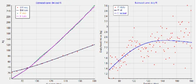
In WP4, the expected feed intake for the next day is estimated by data smoothing techniques processing the recently recorded daily feed intake data. Figure 5 shows measured data on daily feed intake and body weight of a high-performing pig during the growing and fattening period. The left panel of Figure 5 shows the measured daily feed intake and the right panel the body weight recorded on a weekly basis. A much smoother curve can be obtained by visualising and analysing data as the cumulative feed intake. As shown in Figure 6, the cumulative feed intake can be fitted with high accuracy. Using InraPorc, the model predicts both cumulative feed intake and body weight with high accuracy, even though the simulated daily feed intake are in most cases far from the observed feed intake. Therefore, the cumulative feed intake data are more robust as inputs for models in precision feeding systems than the daily feed intake. However, cumulative feed intake is influenced by different animals and environmental factors (e.g., health status, type of diet, temperature).
Page 14/38
Figure 6. Left panel: observed (green dots) and estimated cumulative feed intake (purple line) and observed (red dots) and estimated body weight (black line) of a pig. Right panel: observed (red dots) and estimated (blue line) daily feed intake. The data are the same as those in Figure 5.
Unlike some other models, InraPorc uses a so-called “push approach” for feed and energy intake. This, in combination with an explicit description of protein deposition, makes lipid deposition an energy sink. This approach may be prone to error, because without an explicit control of energy intake, errors accumulate in predicted lipid deposition. Through its association with body water, errors in body protein can be verified (more or less easily and accurately) by measuring body weight. However, errors in body lipid are more difficult to detect. Although backfat thickness is frequently used as an indicator for lipid mass, lipids in backfat represent only about 18% of total body lipids (Kloareg et al., 2006). Because of the potential difficulty of an “uncontrolled” lipid deposition (and without reliable ways to verify it), InraPorc includes a feed intake equation with specific control over energy intake. A Gamma function was proposed in which the ad libitum feed intake is expressed relative to the maintenance energy requirement. During growth, pigs eat above maintenance, but, as they mature, ad libitum feed intake will approach the maintenance energy requirement and the animal will thus stop growing. This concept allows controlling lipid deposition and, if expressed on a cumulative basis, allows representing feed intake as a trajectory to attain. However, in specific conditions the animal may not be able to follow the ideal trajectory of feed or energy intake.
In InraPorc, feed intake is considered a phenotypic trait. As such, it implicitly considers that dietary and environmental factors can modify daily feed intake, but it does not do so explicitly. The feed intake module deals with the estimation of long-term regulation. Determination of feed distribution during the day or feeding patterns as short-term regulators is out of the scope. The long-term regulation of feed intake is complex but, at the same time, energy intake is normally well-regulated in relation to energy expenditure (van Milgen, 2018). However, variation in feed intake is one of the main sources of variation in animal performance. The question as to whether “animals grow because they eat” or “animals eat because they have a desire to grow” has been an issue of discussion among modellers. In many nutritional growth models, feed intake is a model input driving nutrient partitioning. In these “push” models, feed intake is defined by the user or calculated based on the (metabolic) body weight or rate of body weight gain. As discussed earlier, if there is no
Page 15/38
specific control in the model over feed intake, the push approach may lead to erroneous predictions of body composition, especially of body fatness. Feed intake regulation has been considered on an as-fed or on an energy basis. The choice of the type of regulation has an impact on how feed intake (and thus nutrient supply) responds to differences in diet composition. For example, consider two diets with either a high fibre (low energy) content or a high fat (high energy) content. Using a feed intake equation on an as-fed or dry matter basis results in a very different nutrient supply compared with equations based on metabolizable (ME) or net energy (NE). Other factors that affects feed or energy intake include ambient temperature, body composition or composition of body weight gain (i.e., protein and lipid), and water holding capacity or bulk density of the feed (e.g., Nyachoti et al., 2004). It has also been shown that P-deficiency reduces the feed intake appetite of animals. Also factors such as palatability of the feed, social environment, and animal health are known to affect voluntary feed intake, but the quantification of these factors is difficult (Halas et al., 2018). Although feed intake has been considered as phenotypic trait in our approach, we assessed how a number of environmental factors have an impact on feed intake.
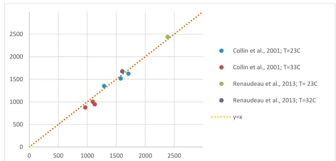
The ambient temperature can have an important impact on the actual feed intake. A number of models are available that quantify effect of the thermal environment on the feed intake response of the animal and these concepts have been integrated in the existing equations of the feed intake module. The sub-model is based on the premise that animal tries to maintain a heat equilibrium. It adjusts its feed intake so that the resulting heat production equals the heat loss. The heat production depends on the maintenance energy expenditure and the inefficiency of nutrient conversions. The heat loss depends on the body surface area and the environmental conditions (e.g., temperature, humidity, air velocity). Behavioural aspects of thermoregulation (e.g., through huddling, changes in physical activity) were not considered here. The model has been challenged with literature data as shown in Figure 7. In the experiment of Collin et al. (2001), growing pigs with a mean body weight ranging from 23 to 32 kg were housed in rooms at either 22 or 32°C. In the experiment of Renaudeau et al. (2013), the same temperature contrast was used for growing pigs (52 and 60 kg BW). The accuracy of model prediction to these data is given in Figure 7.
Figure 7. Comparison of model predictions of daily feed intake with experimental data of from heat stress studies in pigs.
0 500 1000 1500 2000 2500 0 500 1000 1500 2000 2500 Collin et al., 2001; T=23C Collin et al., 2001; T=33C Renaudeau et al., 2013; T= 23C Renaudeau et al., 2013; T=32C y=x
Page 16/38
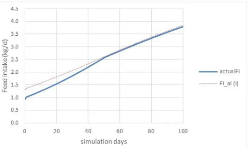
The capacity of the gastrointestinal tract can also be a limiting factor for feed intake. The capacity of the gastrointestinal depends on body weight. However, dietary factors, particularly the so-called water holding capacity (WHC) of the feed, have an impact on the feed intake. A high WHC reduces daily feed intake (Whittemore et al., 2003) and this effect is most pronounced in young animals. Therefore, a high WHC of the feed reduces the feed intake mainly during the growing period. Figure 8 shows an example of a simulation where the WHC is changed from 2.0 to 4.0 g/g (dotted line vs. solid line). Unfortunately, there is very limited information on WHC of different feedstuffs. Mixed feeds composed of conventional ingredients usually have a low WHC (< 2.0) and in this range, the WHC of the feed has no impact on the voluntary feed intake. Feedstuffs that have a high content of soluble non-cellulose polysaccharides (e.g., pea hulls, sugar beet pulp, white lupine, and potato pulp) increase the WHC of the compound feed.
Figure 8. Model simulation on the effect of the water-holding capacity on feed intake in pigs (FI_al(i): WHC = 2 g/g); actualFI: WHC = 4 g/g).
It is well documented that the stocking density has impact on the voluntary feed intake of pigs and poultry, particularly in broilers. The equations used in the model are based on the premise that the energy intake decreases linearly with a reduction of the space allowance compared to the requirement. In the model simulation shown in Figure 9, the red dotted line is the ideal trajectory, while the blue solid line is the estimated daily feed intake if the stocking density is too high. The ideal space allowance is reduced proportionally with time during the fattening period. At the last day of the simulation, the space allowance is only 76% of the ideal situation.
Page 17/38
Figure 9. Effect of a reduced space allowance on the feed intake in pigs. At the end of the simulation with a fixed number of pig per feeder space, space allowance is 76% compared to the ideal situation (actualFI vs FI_al, respectively).
3.4. Layer model
The layer model was not included in deliverable D3.3 and this is the first report on it. An egg production module has been integrated to the re-parameterized broiler model to estimate the impact of nutrient supply on egg production. For re-parametrization, recent literature on growth characteristics and body composition of layers has been used (Nonis, 2007; Nonis and Gous, 2015; Milisits et al., 2016; De Santos et al., 2017; Salas et al., 2018). It is assumed that a laying hen approaches maturity and deposit relatively little body protein. Their protein accretion happens only at the beginning of the laying period, and egg production is a priority.
The hens are characterized by the initial age and body weight, precocity and meanPD (like in the broiler model). The Gamma function for daily feed intake does not seem to be appropriate for a laying period of one year. The Gamma function has been developed for growing animals and is built on the premise that growth ceases at maturity and that animals eat for maintenance then. At the end of the laying period, egg production does not cease in the same way as does growth (i.e., gradually decreasing towards zero). Therefore, an empirical equation to estimate daily feed intake was used as a function of body weight. The disadvantage of an empirical equation is that the function has to be re-parameterized for each genotype. As for the broiler model, the maintenance energy, amino acid, and Ca and P requirements are given first priority, but egg production has priority over the body gain. The Gompertz function determines the body protein deposition (if the amino acid supply is not limiting), and the energy over and above what is required for maintenance, egg production, and body protein deposition is used for body fat deposition. Calcium and P are supplied by the diet, but the skeleton can also serve as a reservoir and can be mobilized (for egg production) up to 50% of its desired mass.
It is clear from the literature that the egg weight depends on genetic factors and is influenced by the nutrient supply. The egg is composed of yolk, albumen, and the shell, and yolk seems to be determining egg size (i.e., egg weight). For simplification, we assumed that yolk weight depends on age, and that the weight of albumen can be described by an allometric function of yolk, and shell weight by an allometric function of yolk plus albumen (Johnston and Gous, 2007). To simulate the impact of nutrient supply on egg weight, it is assumed that the yolk weight, driven by the allometric equation mentioned above, can range ±10% compared to the reference, and thus a minimum and a maximum yolk weight is calculated. The minimum and maximum yolk weight generate a potential minimum and maximum egg weight, and minimum and maximum egg protein mass. The amino acid composition of whole egg and the protein content of each egg component is assumed to be constant. The actual egg weight is the minimum of egg weight allowed by the available amino acid supply (digestible AA amino acid minus the maintenance amino acid requirement) and the genetic potential (determined by protein mass of maximum weight egg). Furthermore, egg shell formation required that sufficient Ca and P are available. If the dietary energy, amino acid, Ca and P supply is insufficient to produce the minimum egg weight, the oviposition is cancelled for that particular day and the nutrients are used for body gain. The energy requirement of egg production is
Page 18/38
calculated based on data of Emmans and Fisher (1986): 1 g of yolk, albumen and shell formation requires 25.0, 1.2, and 3.6 kJ of energy, respectively. The oviposition is also regulated by the age of the hen, the sequence of egg production is calculated based on the egg production rate of the flock.
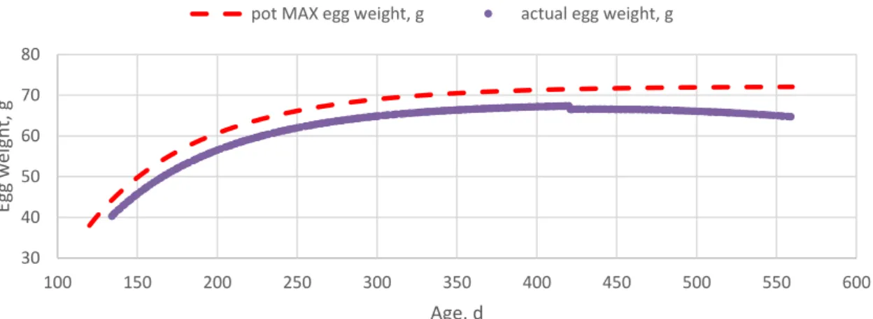
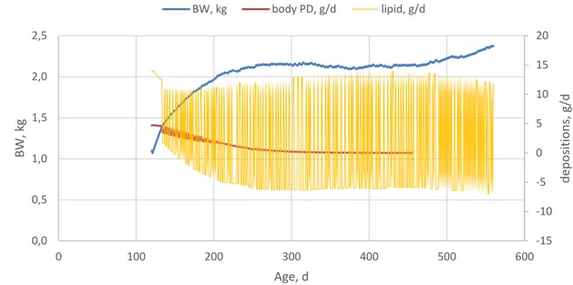
Result of a simulation on egg weight during the laying period as determined by the feed is shown in Figure 10. The nutrients are used for egg formation if there is an oviposition at a certain day. Body fat can be used to cover the energy requirement of the egg production if it is needed, but it can be deposited if there is no egg at a certain day. Therefore, the body composition of a layer dynamically changes over the persistency (Figures 11 and 12).
Figure 10. Simulated egg weight limited by the feed (actual egg weight) and potential maximum egg weight (pot MAX egg weight) over the persistency estimated by the layer model.
Figure 11. Simulated body weight, protein and fat mass of a laying hen over the persistency 30 40 50 60 70 80 100 150 200 250 300 350 400 450 500 550 600 Egg w eight , g Age, d
pot MAX egg weight, g actual egg weight, g
0,00 0,10 0,20 0,30 0,40 0,50 0,60 0,70 0,80 0,0 0,5 1,0 1,5 2,0 2,5 100 150 200 250 300 350 400 450 500 550 600 p ro tein an f fat mas s, kg BW, kg Age, d
Page 19/38
Figure 12. Simulated protein and fat deposition of a laying hen over the persistency.
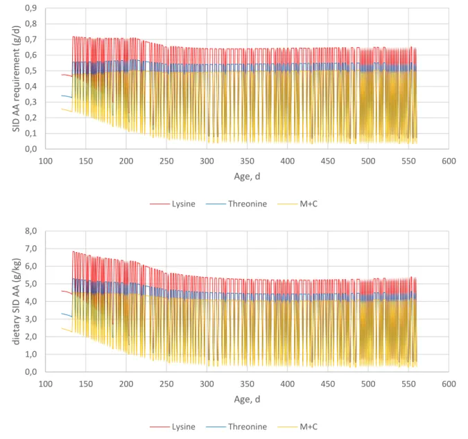
The amino acid requirement of the layers and the optimal standardized ileal digestible amino acid content in the diet are shown in Figure 13. The digestible Ca requirement of the layers are shown in Figure 14.
-15 -10 -5 0 5 10 15 20 0,0 0,5 1,0 1,5 2,0 2,5 0 100 200 300 400 500 600 d ep o sitio n s, g/d BW, kg Age, d BW, kg body PD, g/d lipid, g/d
Page 20/38
Figure 13. Simulated standardized ileal digestible (SID) amino acid requirement (upper panel) and the optimal SID amino acid content of the diet (lower panel) of a layer over the persistency
Figure 14. Simulated digestible Ca requirement of a layer over the persistency 0,0 0,1 0,2 0,3 0,4 0,5 0,6 0,7 0,8 0,9 100 150 200 250 300 350 400 450 500 550 600 SID AA re q u ire m en t (g/ d ) Age, d Lysine Threonine M+C 0,0 1,0 2,0 3,0 4,0 5,0 6,0 7,0 8,0 100 150 200 250 300 350 400 450 500 550 600 d ie ta ry SID AA (g/kg) Age, d Lysine Threonine M+C 0,00 0,50 1,00 1,50 2,00 2,50 3,00 100 150 200 250 300 350 400 450 500 550 600 d igC a re q u ire m en t, g/d Age, d
Page 21/38
4. Conclusions
The above-mentioned models are ready for application in a DSS for precision livestock feeding in different ways: i) the model-generated outputs can be compared with real-time collected data, and ii) the real-time daily, or preferable cumulative feed intake can be used as input in the simulation model to predict the performance for a next period. The difference between the simulation (expected trajectory) and real-time observations can be used as inputs to an early warning system that might be developed to identify technological or health problems. In addition, the concept of the robustness module can also be applied in the DSS developed in task 4.1.
The benefit of using the conceptual models developed in WP3 in a DSS (e.g., in task 4.1) is to provide a more mechanistic approach to estimate the performance of farm animals. Mechanistic models are usually more complicated but can provide more robust predictions over a wider range of conditions compared to statistical or empirical models. Mechanistic models are developed with consideration of biological principles and are generally better functioning in “extreme situation”. The development of decision support tools in farming systems allows that animals (individually or as a group) are fed according to their requirements. By this, nutrients are neither under- nor oversupplied, so that resource efficiency can be maximized, and the environmental footprint is minimized. Also, through the development of an early warning system, animal welfare can be improved.
References
Bibby J., Toutenburg H. (1977). Prediction and improved estimation in linear models John Wiley & Sons, Chichester, UK
Collin A., van Milgen J., Dubois S., Noblet J. (2001). Effect of high temperature on feeding behaviour and heat production in group-housed young pigs. British Journal of Nutrition 86: 63-70.
Emmans G.C., Fisher C. (1986). Problems in nutritional theory. In: Nutrient requirements of poultry and nutritional research (Fisher C., Boorman K.N., eds). pp. 9-39. Butterworths, London.
Halas V., Gerrits W.J.J., van Milgen J. (2018). Models of feed utilization and growth for monogastric animals. In: Feed evaluation science (Moughan P., Hendriks W.H., eds). pp. 423-456. Wageningen Academic Publishers.
Johnston S.A., Gous R.M. (2006). Modelling egg production in laying hens. In: Mechanistic modelling in pig and poultry production (Gous R.M., Morris T.R., Fisher C., eds).pp. 229-259. CABI, Wallingford, UK.
Meda B., Quentin M, Lescoat P., Picard M., Bouvarel I., (2015). INAVI: a practical tool to study the influence of nutritional and environmental factors on broiler performance. In: Nutritional modelling for pigs and poultry (Sakomura N.K., Gous R.M., Kyriazakis I., Hauschild L., eds). pp. 106-124. Cabi, Wallingford, UK.
Milisits G., Szentirmai E., Donkó T., Budai Z., Ujvári J., Áprily S., Bajzik G., Sütő Z. (2016). Effect of initial body weight and body composition of Tetra SL laying hens on the changes in their liveweight, body fat content, egg production and egg composition during the first egg-laying period. Acta Agraria Kaposváriensis 20: 27-35.
Nonis M.K. (2007). Modelling nutrient responses and performance of broiler breeders after sexual maturity (Doctoral dissertation) in Animal and Poultry Science School of Agricultural Sciences and Agribusiness University of KwaZulu-Natal Pietermaritzburg.
Page 22/38
Nonis M.K., Gous R.M. (2015). Changes in the feather-free body of broiler breeder hens after sexual maturity. Animal Production Science 56: 1099-1104.
Nyachoti C.M., Zijlstra R.T., de Lange C.F.M., Patience J.F. (2004). Voluntary feed intake in growing-finishing pigs: A review of the main determining factors and potential approaches for accurate predictions. Canadian Journal of Animal Science 84: 549-566.
Renaudeau D., Frances G, Dubois S., Gilbert H., Noblet J. (2013). Effect of thermal heat stress on energy utilization in two lines of pigs divergently selected for residual feed intake. Journal of Animal Science 91: 1162–1175.
Salas C., Ekmay R.D., England J., Cerrate S., Coon C.N. (2018). Effect of body weight and energy intake on body composition analysis of broiler breeder hens. Poultry Science 98: 796-802.
Santos A.L., De Faria D.E., De Oliveira R.P., Pavesi M., Rizzo Silva M.F., Buranelo Toral F.L., de Lima C.G., Amorim A.B., Dib Saleh M.A., Ramos A.C., Buxade Carbo C. (2017). Growth and body composition of laying hens under different feeding programs up to 72 weeks. Journal of Animal Science and Research 1: 1-6 (doi: 10.16966/2576-6457.103). van Milgen J., Valancogne A., Dubois S., Dourmad J.Y., Sève B., Noblet J. (2008). InraPorc:
a model and decision support tool for the nutrition of growing pigs. Animal Feed Science and Technology 143: 387-405.
Whittemore E.C., Emmans G.C., Kyriazakis I. (2003) The relationship between live weight and the intake of bulky foods in pigs. Animal Science 76: 89-100.
Page 23/38
Appendix 1Matlab code of the P module, FA module, and FI module % ---% initial version
%%%%%%%%% InraPorc-Matlab %%%%%%%%% Date : noivembre 2015
%%%%%%%%% Author : Masoomeh Taghipoor % ******************* % VERSION 05112015 % ******************* % % 0. modified version of 271015 %
% 1. ModeF --> for the situation of the end of simulaton % ModeProfil ---> for the situation of B Gompertz calculation %
% 2. NeintakeSim is replaced by (PDfreeNEintake + PD*GEprotJaap) %
% 3. ag_al et bg_al are now calculated from FI50 and FI100 %%%%%%%%%%%%%%%%%%%%%%%%%%%%%%%%%%%%%%%%%%%%%%%%%%%%%%%%%%%%%%%%% %
% modified by György Kövér 2016-2019 %
% based on P and FI module of Veronika Halas
% based on FA module of Rosil Lizardo and Nuria Tous % ---
% Deliverable D3.1 contains the code of InraPorc-Matlab, just the new modules are provided here
clear all;
InraporcModDuration
function InraporcModDuration % maximum interval of duration
max_duration = 140; % days
% preallocation
BW = zeros(1,max_duration); eBW = zeros(1,max_duration); Prot = zeros(1,max_duration);
BoneP_mass = zeros(1,max_duration); potBoneP_mass = zeros(1,max_duration); total_BoneP_ret = zeros(1,max_duration);
total_P_ret = zeros(1,max_duration); total_surlpus_P = zeros(1,max_duration); Lip = zeros(1,max_duration);
NEint_al = zeros(1,max_duration); FI_al = zeros(1,max_duration); NE_FIal = zeros(1,max_duration);
FI_actual = zeros(1,max_duration); NE_FIactual = zeros(1,max_duration);
Metdig = zeros(1,max_duration); Metm = zeros(1,max_duration); Cysdig = zeros(1,max_duration); Cysm = zeros(1,max_duration);
Trpdig = zeros(1,max_duration); Trpm = zeros(1,max_duration); Thrdig = zeros(1,max_duration); Thrm = zeros(1,max_duration);
Phedig = zeros(1,max_duration); Phem = zeros(1,max_duration); Tyrdig = zeros(1,max_duration); Tyrm = zeros(1,max_duration);
PD_MetCys = zeros(1,max_duration); PD_PheTyr = zeros(1,max_duration); PD_AA_allowed = zeros(1,max_duration);
FHP_al = zeros(1,max_duration); FHP_actual = zeros(1,max_duration); NEm_al = zeros(1,max_duration);
NEm_actual = zeros(1,max_duration); x_AL = zeros(1,max_duration); x_actual = zeros(1,max_duration);
PotPD = zeros(1,max_duration); PotPD_EN = zeros(1,max_duration); mPD = zeros(1,max_duration);
F = zeros(1,max_duration); PDmaxE_AL = zeros(1,max_duration); PDE_Actual = zeros(1,max_duration);
PD_AAfree = zeros(1,max_duration); PD = zeros(1,max_duration); PD_beforeP = zeros(1,max_duration);
ExcessProt = zeros(1,max_duration); ObligUrinELoss = zeros(1,max_duration); UrinE = zeros(1,max_duration);
MEexcessProt = zeros(1,max_duration); NEexcessProt = zeros(1,max_duration); PDfreeNE = zeros(1,max_duration);
PDfreeNEintake = zeros(1,max_duration); NEintakeSim = zeros(1,max_duration); PDfreeNEPD = zeros(1,max_duration);
Page 24/38
PDfreeNEreq = zeros(1,max_duration); EnergyLD = zeros(1,max_duration); LD = zeros(1,max_duration); PD_AA =zeros(12,max_duration); % P module Total_P_int_day = zeros(1,max_duration); AD_P_int_day = zeros(1,max_duration); F_endoP_ex_day = zeros(1,max_duration); P_abs_day = zeros(1,max_duration); U_endoP_ex_day = zeros(1,max_duration); Main_P_day = zeros(1,max_duration); pot_muscle_PD_day = zeros(1,max_duration); LM_mass_day = zeros(1,max_duration); BF_mass_day = zeros(1,max_duration); muscle_dep_day = zeros(1,max_duration); BF_dep_day = zeros(1,max_duration); Ca_abs_day = zeros(1,max_duration); U_endoCa_ex_day = zeros(1,max_duration); Soft_Ca_ret_day = zeros(1,max_duration); BoneP_ret_avCa_day = zeros(1,max_duration); pot_Pret_bone_day = zeros(1,max_duration); relBoneP_def_day = zeros(1,max_duration); maxBoneP_ret_day = zeros(1,max_duration); SoftP_ret_day = zeros(1,max_duration); SoftP_ret1_day = zeros(1,max_duration); BoneP_ret_avP_day = zeros(1,max_duration); BoneP_ret_day = zeros(1,max_duration); act_BoneP_ret_day = zeros(1,max_duration); act_SoftP_ret_day = zeros(1,max_duration); P_ret_day = zeros(1,max_duration); FecalP_ex_day = zeros(1,max_duration); UrineP_ex_day = zeros(1,max_duration); Obl_Urin_P_ex_day = zeros(1,max_duration); surplus_P_day = zeros(1,max_duration); dig_Preq_day = zeros(1,max_duration); P_availability_day = zeros(1,max_duration); digP_utilization_day = zeros(1,max_duration); ratio_of_softP_in_retP_day = zeros(1,max_duration); ret_pr_day = zeros(1,max_duration); ret_pr_2_day = zeros(1,max_duration); Dietary_digP_req_day = zeros(1,max_duration); Dietary_P_req_day = zeros(1,max_duration); muscle_gain_avP_day = zeros(1,max_duration); corr_PD_muscle_avP_day = zeros(1,max_duration); actual_PD_day = zeros(1,max_duration); corr_LD_day = zeros(1,max_duration); FI_actual_not_limited_by_P_intake = zeros(1,max_duration); gBW = zeros(1,max_duration); %FI module E_loss_gas_103 = zeros(1,max_duration); MEI_sim_104 = zeros(1,max_duration); lossE_loss_via_urine_and_gas_105 = zeros(1,max_duration); MEsim_diet_106 = zeros(1,max_duration); NE_181 = zeros(1,max_duration); ME_182 = zeros(1,max_duration); HI_183 = zeros(1,max_duration); THP_184 = zeros(1,max_duration); EHL_min_188 = zeros(1,max_duration); EHL_min_189 = zeros(1,max_duration); T_ambient_194 = zeros(1,max_duration); Water_air_191 = zeros(1,max_duration); humidityFactor_190 = zeros(1,max_duration); Abs_195 = zeros(1,max_duration); EHL_hot_197 = zeros(1,max_duration); EHL_wet_198 = zeros(1,max_duration); EHL_max_199 = zeros(1,max_duration); EHL_max_200 = zeros(1,max_duration);
Page 25/38
SHL_min_205 = zeros(1,max_duration); SHL_max_206 = zeros(1,max_duration); THL_min_208 = zeros(1,max_duration); THL_max_209 = zeros(1,max_duration); THP_210 = zeros(1,max_duration); FI_heatstress_212 = zeros(1,max_duration); FI_coldstress_213 = zeros(1,max_duration); FI_temp_216 = zeros(1,max_duration); en_temp_217 = zeros(1,max_duration); LCT_219 = zeros(1,max_duration); T_220 = zeros(1,max_duration); MaxFI_221 = zeros(1,max_duration); reductMEI_HeatStress_222 = zeros(1,max_duration); Space_req_223 = zeros(1,max_duration); corrMEI_space_225 = zeros(1,max_duration); corrMEI_space_226 = zeros(1,max_duration); corrFI_space_227 = zeros(1,max_duration); FI_bulk_230 = zeros(1,max_duration); actualFI_232 = zeros(1,max_duration); dT_below_LCT_234 = zeros(1,max_duration); dT_below_LCT_NE_235 = zeros(1,max_duration); dT_below_LCT_FI = zeros(1,max_duration); FI_temp_238 = zeros(1,max_duration); actualFI_239 = zeros(1,max_duration); en_actual_240 = zeros(1,max_duration); en_actual_LCT_241 = zeros(1,max_duration); % FA moduleFA_P_subcu = zeros(1,max_duration); FA_P_backf = zeros(1,max_duration); FA_P_inter = zeros(1,max_duration);
FA_P_intra = zeros(1,max_duration); FA_P_muscl = zeros(1,max_duration); FA_P_perin = zeros(1,max_duration); FA_P_other = zeros(1,max_duration);
FA_I_Lipint = zeros(1,max_duration); FA_I_TOTFAint = zeros(1,max_duration); FA_I_C140 = zeros(1,max_duration);
FA_I_C160 = zeros(1,max_duration); FA_I_C161 = zeros(1,max_duration); FA_I_C180 = zeros(1,max_duration);
FA_I_C181 = zeros(1,max_duration); FA_I_C182 = zeros(1,max_duration); FA_I_C183 = zeros(1,max_duration);
FA_I_Other = zeros(1,max_duration); FA_I_Sum = zeros(1,max_duration); FA_I_LipIntCalc = zeros(1,max_duration);
FA_D_Lipint = zeros(1,max_duration); FA_D_C140 = zeros(1,max_duration); FA_D_C160 = zeros(1,max_duration);
FA_D_C161 = zeros(1,max_duration); FA_D_C180 = zeros(1,max_duration); FA_D_C181 = zeros(1,max_duration);
FA_D_C182 = zeros(1,max_duration); FA_D_C183 = zeros(1,max_duration); FA_D_Other = zeros(1,max_duration); FA_D_Sum = zeros(1,max_duration);
FA_E_Lipint = zeros(1,max_duration); FA_E_C140 = zeros(1,max_duration); FA_E_C160 = zeros(1,max_duration);
FA_E_C161 = zeros(1,max_duration); FA_E_C180 = zeros(1,max_duration); FA_E_C181 = zeros(1,max_duration);
FA_E_C182 = zeros(1,max_duration); FA_E_C183 = zeros(1,max_duration); FA_E_Other = zeros(1,max_duration); FA_E_Sum = zeros(1,max_duration);
FA_N_Lipint = zeros(1,max_duration); FA_N_FA = zeros(1,max_duration);
FA_BODYC140 = zeros(1,max_duration); FA_BODYC160 = zeros(1,max_duration); FA_BODYC161 = zeros(1,max_duration);
FA_BODYC180 = zeros(1,max_duration); FA_BODYC181 = zeros(1,max_duration); FA_BODYC182 = zeros(1,max_duration);
FA_BODYC183 = zeros(1,max_duration); FA_BODY_O = zeros(1,max_duration);
FA_N_C140 = zeros(1,max_duration); FA_N_C160 = zeros(1,max_duration); FA_N_C161 = zeros(1,max_duration);
FA_N_C180 = zeros(1,max_duration); FA_N_C181 = zeros(1,max_duration); FA_N_C182 = zeros(1,max_duration);
FA_N_C183 = zeros(1,max_duration); FA_N_Other = zeros(1,max_duration);
FA_B_C140 = zeros(1,max_duration); FA_B_C160 = zeros(1,max_duration); FA_B_C161 = zeros(1,max_duration);
FA_B_C180 = zeros(1,max_duration); FA_B_C181 = zeros(1,max_duration); FA_B_C182 = zeros(1,max_duration);
Page 26/38
FA_B_C183 = zeros(1,max_duration); FA_B_Other = zeros(1,max_duration); FA_B_SUM_FA = zeros(1,max_duration);
FA_IN_body_FA = zeros(1,max_duration); FA_IN_body_C140 = zeros(1,max_duration); FA_IN_body_C160 = zeros(1,max_duration);
FA_IN_body_C161 = zeros(1,max_duration); FA_IN_body_C180 = zeros(1,max_duration); FA_IN_body_C181 = zeros(1,max_duration);
FA_IN_body_C182 = zeros(1,max_duration); FA_IN_body_C183 = zeros(1,max_duration); FA_IN_body_O_FA = zeros(1,max_duration);FA_IN_SUM_body_FA = zeros(1,max_duration);
%Temperatue and humidity parameters in csv file
[numParam, textParam] = xlsread('TempData.csv');
T_ambient_194 = numParam(4,:); % Ambient temperature data expected in raw #2
% size extended by repeating the last value
T_ambient_194 = [T_ambient_194, zeros(1, max_duration - length(T_ambient_194))+T_ambient_194(numel(T_ambient_194))]; Air_speed_192 = numParam(2,:);
% size extended by repeating the last value
Air_speed_192 = [Air_speed_192, zeros(1, max_duration - length(Air_speed_192))+Air_speed_192(numel(Air_speed_192))]; RH_193 = numParam(3,:);
% size extended by repeating the last value
RH_193 = [RH_193, zeros(1, max_duration - length(RH_193))+RH_193(numel(RH_193))]; Space_allowance_224 = numParam(5,:);
% size extended by repeating the last value
Space_allowance_224 = [Space_allowance_224, zeros(1, max_duration - length(Space_allowance_224))+Space_allowance_224(numel(Space_allowance_224))]; WHC_229 = numParam(6,:);
% size extended by repeating the last value
WHC_229 = [WHC_229, zeros(1, max_duration - length(WHC_229))+WHC_229(numel(WHC_229))];
%Parameters Inraporc, P, FI, FA modules
[numParam, textParam] = xlsread('Import_051115PFI',3);
nameP = textParam; valueP = numParam;
%Feed composition
[numFC, textFC] = xlsread('Import_051115PFI',2); nameFC = textFC(2:9,1);
nameFC2 = textFC(1,2:7); valueFC = numFC;
%Import from InraPorc
[numFeed, textFeed] = xlsread('import.csv'); nameFeed = textFeed(1,4:98)';
valueFeed = numFeed(:,2:96)';
Diet = textFeed(2:size(textFeed,1),1)';
%AA = importdata('AA.dat');
[numAA, textAA] = xlsread('Import_051115PFI',1); names = textAA(2:14,1); namesH = textAA(1,2:8); values = numAA; %#################################################### % Model Parameters
% The explication of the parameters and (default)
% numerical values are given in the Excel file,
% that are used as model inputs as in InraPorc_Matlab
%#####################################################
%
% P Model Parameters Veronika Halas
%
DM_P = valueP(ismember(nameP(:,1),'DM') == 1,1); % overwritten later
reabs_feP = valueP(ismember(nameP(:,1),'reabs_feP') == 1,1);
e_P_growth = valueP(ismember(nameP(:,1),'e_P_growth') == 1,1);
P_cont_muscle = valueP(ismember(nameP(:,1),'P_cont_muscle') == 1,1);
P_cont_visc = valueP(ismember(nameP(:,1),'P_cont_visc') == 1,1);
P_cont_fat = valueP(ismember(nameP(:,1),'P_cont_fat') == 1,1);
Ca_cont_muscle = valueP(ismember(nameP(:,1),'Ca_cont_muscle') == 1,1);
Ca_cont_fat = valueP(ismember(nameP(:,1),'Ca_cont_fat') == 1,1);
P_dig = valueP(ismember(nameP(:,1),'P_dig') == 1,1);
Ca_dig = valueP(ismember(nameP(:,1),'Ca_dig') == 1,1);
F_endoP = valueP(ismember(nameP(:,1),'F_endoP') == 1,1);
Page 27/38
U_endoCa = valueP(ismember(nameP(:,1),'U_endoCa') == 1,1);
CaP_ratioBone = valueP(ismember(nameP(:,1),'CaP_ratioBone') == 1,1);
CaProt_ratio = valueP(ismember(nameP(:,1),'CaProt_ratio') == 1,1);
Prot_muscle = valueP(ismember(nameP(:,1),'Prot_muscle') == 1,1);
P_FI_MODULE_ACTIVE = valueP(ismember(nameP(:,1),'P_FI_MODULE_ACTIVE') == 1,1);
%
% Feed intake Model Parameters Veronika Halas
%
HL_slope = valueP(ismember(nameP(:,1),'HL_slope') == 1,1);
BodyTemp_min = valueP(ismember(nameP(:,1),'BodyTemp_min') == 1,1);
BodyTemp_max = valueP(ismember(nameP(:,1),'BodyTemp_max') == 1,1);
dt_below_LCT_NE_const = valueP(ismember(nameP(:,1),'dt_below_LCT_NE_const') == 1,1);
%####################################################
% Initial conditions as in InraPorc_Matlab
%####################################################
% Initial conditions for the P Model Veronika Halas
BoneP_mass(1) = Prot(1)*0.99*CaProt_ratio/CaP_ratioBone; % CaP_ratioBone =
2.2 from parameterfile
potBoneP_mass(1) = Prot(1) * CaProt_ratio *0.99/CaP_ratioBone; % CaProt_ratio = 0.05
from parameterfile
total_BoneP_ret(1) = 0; % P Model
total_P_ret(1) = 0; % P Model
total_surlpus_P(1) = 0; % P Model
% ---
% Lipid mass at the start of the simulation as in InraPorc_Matlab.
%#####################################################%###
% Feed plan sequence as in InraPorc_Matlab
% Select duration or final BW for the end of simulation ModeF as in InraPorc_Matlab % Fatty acid module starts
FA_started=false; % FA mudule is not started yet
diet_diet2=false; % FA module activates in case of feed#2
step = 1;
for i = 1:step : min(Age_final_sim - Age_init +1,max_duration)
%#####################################################
% Feed composition
%#####################################################
%Feed plan sequence
if SFP == 2 && BW(i)>=TC %2 plans
Diet = Diet2; diet_diet2 = true; else Diet = Diet1; diet_diet2 = false; end % FA module
FatT_diet2 = valueFeed(ismember(nameFeed(:,1),'Fat') == 1,Diet); % Crude Fat(%)
FAlipT_diet2 = valueFeed(ismember(nameFeed(:,1),'FA/lipid') == 1,Diet); % Crude
Fat(%)
C140T_diet2 = valueFeed(ismember(nameFeed(:,1),'C14:0') == 1,Diet); % Crude Fat(%)
C160T_diet2 = valueFeed(ismember(nameFeed(:,1),'C16:0') == 1,Diet); % Crude Fat(%)
C161T_diet2 = valueFeed(ismember(nameFeed(:,1),'C16:1') == 1,Diet); % Crude Fat(%)
C180T_diet2 = valueFeed(ismember(nameFeed(:,1),'C18:0') == 1,Diet); % Crude Fat(%)
C181T_diet2 = valueFeed(ismember(nameFeed(:,1),'C18:1') == 1,Diet); % Crude Fat(%)
C182T_diet2 = valueFeed(ismember(nameFeed(:,1),'C18:2') == 1,Diet); % Crude Fat(%)
C183T_diet2 = valueFeed(ismember(nameFeed(:,1),'C18:3') == 1,Diet); % Crude Fat(%)
% P model Veronika Halas
DM_P = valueFeed(ismember(nameFeed(:,1),'DM') == 1,Diet)*1E-3;% Dry matter (%) %
overwrites the param file value
dietary_Ca = valueFeed(ismember(nameFeed(:,1),'Ca') == 1,Diet);% dietary_Ca (%)
dietary_P = valueFeed(ismember(nameFeed(:,1),'P') == 1,Diet); % dietary_P(%)
% Original InraPorc_Matlab to calculate digestible nutrient & DE & ME & NE content
Page 28/38
%** Import of AA data as in InraPorc_Matlab
%%#####################################################
% dietary AA composition and SID AA intake, AA metabolism as in InraPorc_Matlab
% NE intake calculation as in InraPorc_Matlab
NEint_al(i) = (ag_al*bg_al*BW(i)*exp(-bg_al*BW(i))+1)*0.75*BW(i)^(0.6);%(MJ/d) %
starting value for the optimization
%
also the calculated value without the Temperature module
options = optimset('Algorithm','levenberg-marquardt','Display', 'notify'); if P_FI_MODULE_ACTIVE==1 y=lsqnonlin(@InraporcModDay,NEint_al(i), [], [], options); else yo=InraporcModDay(NEint_al(i)); end end i % nested function
function fobj = InraporcModDay(x) %fobj =
%%#####################################################
%** Ad Lib feeding from InraPorc
%%#####################################################
%i
% Ad libitum NE intake MJ/d
% NEint_al(i) = a_al*(BW(i))^b_al;%(MJ/d)
%Parameters of Gamma function
% cGammaFrais = 0.075; % cGammaMS = 0.066; % cGammaED = 1.04; % cGammaEM = 1.00; % cGammaEN = 0.75; % dGamma = 0.60; % NEint_al(i) = (ag_al*bg_al*BW(i)*exp(-bg_al*BW(i))+1)*0.75*BW(i)^(0.6);%(MJ/d) NEint_al(i) = x;
% Ad libitum feed intake
FI_al(i) = NEint_al(i)/NE; %(kg/d)
% Ad libitum NE intake in kJ/d
NE_FIal(i) = NEint_al(i) * 1E+3;%(kJ/d)
% actual feed intake taking into account rationing rate
FI_actual(i) = FI_al(i) * rate_ratio;
% actual NE intake
NE_FIactual(i) = 1E+3*FI_actual(i) * NE; %(kJ/d)
% AA intake, per considered AA
AAdig_intake(:,i) = AA_DigContent * FI_actual(i) * 1E+1;%g
% Maintenance AA requirement, per AA
AA_m(:,i) = AAm75 * BW(i)^0.75 + FI_actual(i) * (DM/100) * AA_endog;%g
% PD allowed by the AA supply, per AA as in InraPorc_Matlab
% energy metabolism as in InraPorc_Matlab
% --- Beginning of P Model
% PD can be limited by dietary P content
% Veronika Halas
% --- The init part is NOT HERE, moved after the BW init
% BoneP_mass(1) = Prot(1)*0.99*CaProt_ratio/CaP_ratioBone; %
CaP_ratioBone = 2.2 from parameterfile
% potBoneP_mass(1) = Prot(1) * CaProt_ratio *0.99/CaP_ratioBone; % CaProt_ratio =
0.05 from parameterfile
% --- init end
Total_P_int = FI_actual(i) * dietary_P; % total P intake (34)
AD_P_int = FI_actual(i) * dietary_P * P_dig; % apparent digestible P supply (35)
F_endoP_ex = F_endoP * DM_P*FI_actual(i); % fecal endogenous P