IN GENERAL INSURANCE BY
ROBERT SALZMANN, MARIO V. WÜTHRICHAND MICHAEL MERZ
ABSTRACT
The claims development result (CDR) is one of the major risk drivers in the profi t and loss statement of a general insurance company. Therefore, the CDR has become a central object of interest under new solvency regulation. In current practice, simple methods based on the fi rst two moments of the CDR are implemented to fi nd a proxy for the distribution of the CDR. Such approxima-tions based on the fi rst two moments are rather rough and may fail to appro-priately describe the shape of the distribution of the CDR. In this paper we provide an analysis of higher moments of the CDR. Within a Bayes chain ladder framework we consider two different models for which it is possible to derive analytical solutions for the higher moments of the CDR. Based on higher moments we can e.g. calculate the skewness and the excess kurtosis of the distribution of the CDR and obtain refi ned approximations. Moreover, a case study investigates and answers questions raised in IASB [9].
INTRODUCTION
One of the most important fi nancial positions in the balance sheet of a general insurance company are the claims reserves. The claims reserves are used for paying the outstanding loss liability cash fl ows. The changes (over time) in these claims reserves, called the claims development result (CDR), are one of the major risk drivers in the profi t and loss statement of a general insurance com-pany. Therefore, in new solvency regulations, such as Solvency II, the CDR has become a central object of interest for the assessment of the reserving risk. As proposed in Solvency II and applied in current practice, a proxy for the distribution of the CDR is obtained by fi tting a shifted lognormal distribution to the estimates of the fi rst two moments of the CDR. This rather rough approach may fail to describe the shape of the distribution of the CDR. In fact, fi tting a shifted lognormal distribution to the fi rst two moments or applying bootstrapping techniques often lead to rather symmetric approximations to the distribution of the CDR which, in general, fail to fi t the skewness and the excess kurtosis of the distribution of the CDR. Knowledge about the shape
of the distribution is important for the risk assessment of future cash fl ows as discussed in IASB [9]. As for instance stated in paragraph B76 of IASB [9], for the selection of the confi dence level for estimating risk adjustments the insurer must take into account additional factors, such as the skewness of the probabil-ity distribution. Moreover, when it comes to selecting an appropriate technique to estimate risk adjustments, shape parameters such as the skewness have to be taken into account as stated in paragraph B95 of IASB [9]. The considera-tion of higher moments allows insurance companies to gain more insight into the shape of the distribution of the CDR which is essential for the application of techniques for estimating risk adjustments as discussed in IASB [9].
We work within a chain ladder (CL) framework. Since the CDR in the next accounting year results from an information update, such problems are most naturally understood recursively (see Bühlmann-Gisler [2], Section 9.2). A uni-fi ed approach to incorporate new information into a CL model is provided by the Bayes CL framework (see Bühlmann et al. [1]). In this paper we con-sider two different distributional Bayes CL models. We emphasize that for the analysis of higher moments we need to make explicit distributional model assumptions.
As an important property of the Bayesian setup we highlight that it does not only allow for the incorporation of the information update but it also accounts for the parameter estimation uncertainty in a natural way. Moreover, our distributional model assumptions allow for the calculation of higher moments of the CDR in closed form w.r.t. the data available.
In a case study we fi t the so called 4-parameter Johnson family of distribu-tions (see Johnson et al. [11]) to moments up to order four of the CDR, i.e. in addition to the fi rst two moments we fi t the skewness and excess kurtosis of the CDR. As a special case the 4-parameter Johnson family of distributions includes the shifted lognormal distribution which is proposed in Solvency II as a proxy for the distribution of the CDR. This allows to directly compare the distributional approximation for the shifted lognormal distribution based on the fi rst two moments with the refi ned approximation for the 4-parameter Johnson family of distributions based on higher moments up to order four. The case study shows that considering the shape of the distribution of the CDR signifi cantly infl uences the uncertainty analysis of the CDR and answers questions raised in IASB [9].
Organization of the paper
In the following section we introduce the CDR. In Section 2 we defi ne two different Bayes CL models. Then we calculate posterior distributions (of the underlying model parameters) which enable us to compute higher moments of the CDR in closed form (as far as they exist) for single accident years as well as for the aggregated case, see Section 3. The estimation of the structural param-eters (which are needed to calibrate the models) is described in Section 4. Finally, Section 5 presents a case study and a discussion of the results. The main results are proved in the appendix.
FIGURE 1: Information update DI " DI + 1 during the fi rst accounting year (0,1], a new diagonal
is added to the trapezoid at the end of accounting year 1. 1. CLAIMS DEVELOPMENT RESULT
In the sequel we work with claims development triangles (trapezoids) for which the single entries correspond to cumulative claims denoted by Ci, j > 0.
The index i ! {0, …, I} refers to accident years and the index j ! {0, …, J} to development years (I $ J). We assume that the ultimate claim for accident year
i ! {0, …, I} is given by Ci, J. This means we assume that there is no
develop-ment after developdevelop-ment year J.
At time I + t, t $ 0, we have observations denoted by
; , , .
C i j I t 0 i I 0 j J
DI+t = $ i j, + # + # # # # .
This corresponds to the runoff situation because no new accident years i are added to DI + t after year I. The period (t – 1, t] is called accounting year t and
DI + t is the information available at the end of accounting year t.
Claims reserving is basically a prediction problem and we are mostly inter-ested in the prediction of the ultimate claim Ci, J. The Bayesian predictor for
the ultimate claim Ci, J, given DI + t, is defi ned by ,
i J i J,
C = EC DI+t .
( )t 8 B (1.1)
Note that this predictor is unbiased and has minimal (conditional) L2 -uncer-tainty among all DI + t-measurable predictors and is therefore often called
“best-estimate” predictor.
The difference in successive ultimate claim predictions resulting from an information update DI " DI + 1, see Figure 1, determines the CDR in the fi rst
accounting year (0,1].
Defi nition 1.1. The CDR for accident year i = I – J + 1, …, I in the fi rst accounting year is defi ned by
, ,
iJ iJ
i C C
For a further description we refer to Section 3 in Bühlmann et al. [1]. Making use of the martingale property of successive ultimate claim predictions (under the assumption that the fi rst moments exist) we obtain from (1.1)
i
CDR 0.
E
6
DI@
=Therefore, in the profi t and loss statement the CDR is predicted by zero. The pre-diction variance (conditional mean square error of prepre-diction) is given by, see Wüthrich-Merz [16],
CDR CDR
i
msepCDR|DI(0) = E9_ i-0i2 DIC = Var_ i DIi.
The prediction variance is probably one of the easiest risk measures that can be calculated. An analytical formula for this second moment is derived in Bühlmann et al. [1]. For gaining more insight into the distribution of the CDR we aim to calculate higher moments of this CDR.
2. BAYES CHAIN LADDER MODELS
In this section we consider two different distributional models for the Bayes CL model. Both models are such that the distributions belong to the exponential dispersion family with associate conjugate priors (see e.g. Bühlmann-Gisler [2]). This choice allows for closed form solutions for posterior distributions. To begin, we defi ne the individual claims development factors by
j j 1 , F C C j = + , i , i , i
for i ! {0, …, I} and j ! {0, …, J – 1}. The cumulative claims Ci, j are then given
by F 1 = i, , C C i k, k j 0 0 = , i j +
%
where Ci, 0 refers to the initial value of the stochastic process (Ci, j )j = 0, …, J and
the Fi, j’s describe the individual multiplicative changes from development year
to development year. Next, we defi ne the two different distributional models for the individual claims development factors Fi, j. First, we study the
Gamma-Gamma Bayes CL model also considered in Salzmann-Wüthrich [15].
2.1. Gamma-Gamma Model
Model 2.1. (Gamma-Gamma Model)
(a) Conditionally, given Q = (qj)0 # j # J – 1, (Ci, j)j $ 0 for i = 0, …, I are
independ-ent Markov processes with conditional distributions
, j2 j j2 - -j j 1 j + . F C C , , i j Ci, +G c c = Q , , i i q a k
(b) qj are independent G(gj, fj(gj – 1))-distributed with given prior constants fj > 0, gj > 1.
(c) Q and Ci, 0 are independent and Ci, 0 > 0, P-a.s.
¡
Remark. The gamma distribution is denoted by G(g, c). In particular for X +
G(g, c) with g, c > 0 we have that E[X ] = g/c and Var(X ) = g/c2. The gamma
distribution has the following moments:
X -k k ( ) ( ) c E k = G +g G g ,
6 @
(2.1)for k ! Z with – k < g and G(x) denotes the gamma function. This determines for which k the moments of X exist.
Under Model 2.1 we have the following properties:
(2.2) j j j Var j j 1 , i j j j j j j j j j j 1 1 + + , Var . C C C F C C C C C F C C E E , i 2 2 c = = = = -q q , , , , , , , , , , i i i i i i i i i2 i , , , , Q Q Q Q 2 a k ` j 8 B 8 B (2.3) Remarks.
• From formula (2.2) we see that qj –1 plays the role of the development factor
(see Mack [12]). The variance (2.3) is quadratic in the observation an there-fore our assumptions differ from the classical distribution-free CL model of Mack [12]. As a consequence there is no prior difference in risk w.r.t. the volume between two different portfolios having the same prior parameters cj and qj. Furthermore, the conditional coeffi cient of variation is given by
j C j j. j j j j 1 1 1 , Q + + + Vco C | Var C C C C E = = , , , , , , i i i i i i c / 1 , , Q Q 2 ` j ` j 8 9 B C
• The assumptions on the distributions of the qj’s refl ect our prior knowledge
about the true parameters. For gj " 1 we are in the non-informative case
where we have no prior knowledge. Note that we need gj > 2 for the prior
2.2. Lognormal-Normal Model
Secondly, we consider a lognormal distribution for the individual development factors Fi, j and for the prior distribution we choose a normal distribution.
Model 2.2. (Lognormal-Normal Model)
Assume that sj2 > 0, j = 0, …, J – 1 are given fi xed constants.
(a) Conditionally, given m = (mj)0 # j # J – 1, (Ci, j)j $ 0 for i = 0, …, I are
independ-ent Markov processes with conditional distributions
j L j j 1 j j , . F C C 2 , i ( + = N m s , , , i i i j + ) , m C
(b) mj are independent N(zj, nj2)-distributed with given prior constants zj and nj > 0.
(c) m and Ci, 0 are independent and Ci, 0 > 0, P-a.s.
Remarks.
• LN( m, s2) denotes the lognormal distribution and N( m, s2) the normal dis-tribution.
• Model 2.2 inherits similar features as Model 2.1 since there is no volume term Ci, j in the distribution of the Fi, j. The only modifi cation is that we have
different distributional assumptions.
• In Model 2.1, the gamma distributed parameter qj enters the model
recipro-cally (c.f. (2.2)-(2.3)). We know that inverse gamma distributions lie in the Fréchet maximum domain of attraction (see McNeil et al. [14]). Therefore they belong to the family of heavy-tailed distributions with infi nite higher moments. As a consequence, this may lead to heavy-tailed distributions for the CDR w.r.t. DI for Model 2.1, i.e. higher order moments thereof may not
exist. On the other hand, as we will see in Section 3 all moments exist for the distribution of the CDR w.r.t. DI resulting from the lognormal distribution
of Model 2.2. We refer to such distributions as being moderately heavy-tailed, see also McNeil et al. [14].
• The structural parameters cj and sj are assumed to be fi xed constants,
see Model 2.1 and Model 2.2. Only this assumption will allow for closed form solutions for higher moments of the CDR. We will derive and discuss plug-in estimators for these structural parameters in Section 4.
• Similar to Model 2.1, letting nj " 3 corresponds to the non-informative
case, i.e. we have no prior knowledge about the parameter mj.
Under Model 2.2 we have the following properties:
j/ s + j+1 j j j jexp 2 C C C F C C E
6
i, m, i,@
= i, E6
i j, m, i,@
= i, amj 2 k, (2.4)j j j
C,
j+1 j i
Var`Ci, m,Ci,j = 2 expa2mj+s2k`exp(s2)-1j, (2.5)
j
j+1 j
Vco`Ci, |m,Ci,j = aexp(s2)-1k1 2/ . (2.6)
Unlike qj in Model 2.1, mj is not directly associated with the CL factor which
is now given by exp (mj + sj2/2), (c.f. (2.4)) and thus depends on sj.
3. POSTERIOR DISTRIBUTIONSAND HIGHER MOMENTS
In this section we are going to exploit the recursive structure (see Bühlmann et al. [1]) of the different Bayes CL models presented in Section 2 in order to fi nd closed form solutions for higher moments of the CDR, fi rst for single accident years and second for the aggregated case.
3.1. Posterior Distributions
Since Model 2.1 and Model 2.2 belong to the exponential dispersion family with associate conjugate priors, the Bayesian estimators coincide with the linear credibility estimators (exact credibility case). Moreover, it is possible to explic-itly calculate the posterior distributions of Q and m, given DI + t. In the same
spirit of Theorem 3.2 of Gisler-Wüthrich [6], we state the following proposition for the two different models. The proofs are provided in the appendix.
Proposition 3.1 (Exact Credibility Case). (a) Under the assumptions of Model 2.1,
given DI + t with t = 0, 1, the posterior distributions of Q = (qj)0 # j # J – 1 are
inde-pendent gamma distributions with parameters
j j j , , j j t j + -t t 2 2 ( ( 1) . I j c fj C i I j t 0 1 c c = - + = + = - - + g g , i j+1 ), -g
/
(b) Under the assumptions of Model 2.2, given DI + t with t = 0, 1, the posterior
distributions of m = (mj)0 # j # J – 1 are independent normal distributions with
parameters j j j , j j j t j j j 2 2 2 -, i j ( , j t i=0 log ) I j t F I j t 1 1 I j 1 t z = z + - + + = + - + - - + n s n s n n s n 2 2 2 2 . 2 , ^ ^ h h
/
3.2. Credibility CL Factors
This section revisits important results needed for the calculation of higher moments of the CDR.
3.2.1. Gamma-Gamma Model
For Model 2.1, Proposition 3.1 implies for i > I – J + t that
j , i , j J E t E j I+t i, 1 I+t i, C C C C c . 1 D D , j I i t J j j I i t J 1 1 = = = -= - + -= - + -, i q t I- +i t I- +i t ( )t g 6 @
%
9 C%
(3.1)Defi ne the posterior estimates of the CL factors for j = 0, …, J – 1 by Fj(t) =
E [qj– 1| DI + t ]. From straightforward calculation we obtain the following
corollary:
Corollary 3.2. Assume Model 2.1, then for t # j # J – 1 with t = 0, 1 the posterior
estimates Fj(t) are given by the weighted average
j j, aj,t j F( )t = a t fj t, +(1- ) f, (3.2) for t = 0,1 with i=0 F , , j t i j = I- - +j 1 t I- +j t , f
/
and credibility weight at time I + t
j , j t a ( 1). I j t I j t j c = - + + -- + 2 g (3.3)
Remark. The estimator fj, t corresponds to the maximum likelihood estimator
(MLE) of qj – 1 at time I + t.
Similar to Theorem 2.1 in Bühlmann et al. [1] we obtain for the posterior estimates of the CL factors in the Gamma-Gamma model the recursive struc-ture for the updating procedure.
Corollary 3.3. Assume Model 2.1, then for 1 # j # J – 1
j
j I-j j, +
F( )1 = bjF `1-bjjF( )0,
with DI -measurable credibility weight
j 1 ( 1). I j 1 j j c = - + + 2 -b g (3.4)
3.2.2. Lognormal-Normal Model
Analogous results hold true for Model 2.2, if we defi ne Yi, j = log Fi, j =
log(Ci, j + 1 /Ci, j ) and Yj(t) = E[mj|DI + t]. Given m and Ci, j, we see that Yi, j is
normally distributed with Yi, j |m,Ci, j + N(mj, sj) which immediately implies the next corollary.
Corollary 3.4. Assume Model 2.1, then for t # j # J – 1 with t = 0,1 the posterior
estimates Yj(t) are given by the weighted average
j j j t, rj,tY ( rj,t) j Y( )t = z = ( )t + 1- z , (3.5) with Y j j , j , j j j t j ( at ) + -Y ( ) ) . I j t MLE time I t j t I j t
credibility weight at time I t
1 1 , i j i I j t 0 1 ( ) r = - + + = - + - + + = - - + m n s n s 2 2 -I 2 2 of ( )t (
/
(3.6)Moreover, we obtain the following recursive structure in this case.
Corollary 3.5. Assume Model 2.2, then for 1 # j # J – 1
j j I-j, j j
Y( )1 = k Y j+(1-k)Y( )0,
with credibility weight
j j j j 1 -1 (I j ) . j = + - + n s n s 2 2 2 2 k (3.7)
Due to the assumptions of Model 2.2 and the posterior independence of the parameter m = (mj)0 # j # J – 1 according to Proposition 3.1 we thus obtain
(3.8) j j , i , j t J , j t + C j C . exp exp exp C C 2 2 2 E D , E D , I t i I i t j I i t J j I t i I i t j I i t J 1 2 1 2 z = = + = + - + = - + -+ - + = - + -m s n s , i 2 ( )t e e e o o o 9 C
%
>
H
%
(3.9)Moreover, with Corollary 3.5 we get
j Y +(1-k)Y j j , I-j j , j 1 j j
F E exp j 2 DI exp j exp 2 2 .
2 1 2 = + + = + s k s n ) 2 1 ( m ( )0 c m a k c m
>
H
(3.10)Note that in the above formula YI – j, j is the only term which is not DI
-meas-urable.
3.3. Higher Moments Single Accident Years
Proposition 3.1, Corollary 3.3 and Corollary 3.5 allow for the calculation of higher moments of the ultimate claim predictor Ci J,
( )1 given D
I for both models. Proposition 3.6. Choose i > I – J.
(a) Assume Model 2.1 and let Ni = min{gI – i, 0, …, gJ – 1, 0}. For n ! N with n < Ni we obtain j , i J 1 j j l n , i I-i C C K K 1 F , E DI n, , l n l j n l j I i J 0 1 = -= -= - + -l n n l ) - ) b b n 1 0 ( I-i ( a k ` j b l^ h ^ h a k ; E
%
;/
Ewhere credibility weight bj is given by (3.4) and for j = I – i, …, J – 1 and 0 # l # n
j j -l j l + , , j j 0 0 -, j 0 2 2 ( ) ( ) Kl j, c c c c = 2 l G G G G g g , a a a k k k
with cj, 0 and gj, 0 given by Proposition 3.1.
(b) Assume Model 2.2. We obtain , i J i, j C C exp n M E n DI , , j I i J j n 1 0 = = -I-i ) , 1 z ( n ` j ^ h : D
%
with j j 2 2 , , j0 j1 j j ( ) ( ) , exp M n n n 2 2 2 2 , { } n j j I i 2 2 2 > = + + + -s n2 s n k k 1 e f o pwith zj, 0 and nj, t given by Proposition 3.1 and kj given by (3.7) for j > I – i and
kI – i = 1.
Remarks.
• In Proposition 3.6 we calculate moments of Ci J,( )1 given DI. To get moments of
CDRi we have to consider moments of Ci J, ( )0 – , i J C( )1. Since , i J C( )0 is D I
-measur-able this can be done easily. For instance, the second moment of CDRi is
given by
E CDRi2 DI E Ci,J Ci,J DI E Ci,J DI Ci,J .
2 2
= a (0)- (1)k = a (1)k -a (0) 2k
Therefore, moments of CDRi given DI are determined by moments of Ci J, ( )1.
• Moreover we can calculate the skewness and excess kurtosis of CDRi. In
the case study in Section 5 we change signs for the CDR such that losses in the CDR correspond to positive values (and are in-line with the classical defi nition of risk measures). Therefore, the skewness and excess kurtosis thereof are given by
skewness = 2 3 i i CDR CDR E E I I -3 D /2 D ^
6
h6
@
@
, excess kurtosis = 4 i i CDR CDR 3. E E I I 2 -D D 2 ^6
h6
@
@
Note that the moments in the above formulas for the skewness and the excess kurtosis are moments relative to the mean which in our case is given by E[CDRi|DI] = 0.
• Skewness smaller than zero may indicate distributions with heavier left tail than right tail whereas skewness greater than zero may indicate that the right tail is heavier. Excess kurtosis measures the excess of the kurtosis over the kurtosis of a normal distribution. Excess kurtosis greater than zero indicates that the distribution is more peaked and has a heavier tail than a normal distribution.
Linear combinations of independent normally distributed random variables are again normally distributed. It is therefore possible for Model 2.2 to get a closed form solution for the distribution of Ci J,( )1, given m and D
I, according to the
following proposition.
Proposition 3.7. Choose i > I – J. Assume Model 2.2. Conditionally, given m and DI, Ci J,
( )1 has the following distribution
k m , j j , iJ m,D j j C | LN di , j I i J j I i J 1 2 1 2 I + = = -s k ) 1 ( + f
/
/
pwith kj given by (3.7) for j > I – i and kI – i = 1 and
j (F )+ j j 1 ( j , j j 1 + 1 -i ( ) . log log d C 1 2 2 , { } , i I i j k I j k j j I i J 0 1 2 1 1 = + + + + -= -= - + -n s s n 2 -k I 2 2 z i I> - +J 1 )
f
/
p
/
3.4. Higher Moments Aggregated Accident Years
To study uncertainties in the CDR for aggregated accident years, we consider moments of C:,J ( )1 defi ned by , i ,J CJ C . i I J I 1 : = - + ) ( )1 (1 =
/
The following theorem gives closed form solutions for both models.
Theorem 3.8. For n ! N and k0, …, kJ – 1 ! {0, 1, …, n} defi ne hs =
/
us=0ku(a) Assume Model 2.1. For n < min{g0, 0, …, gJ – 1, 0} we obtain
J- -1 s J- -1 s , CI- + +J 1 s, ! J s 1 b h : r C , , , ( ) , n k k k K E , , , , , n I J h n k k n s J s J r n h J s r r s 0 1 1 0 0 1 1 0 1 J J s s s s 1 0 # f = -f f -= -= -= -- -- + -- ) -k D J 0 1 -( ) 1 h 1 F k n -n br ( a e a d ` j o n j p : D " ,
%
/
/
where Kl, j are given by Proposition 3.6 (a), bj is given by (3.4) and the last sum
is set equal to Kks, J – 1 – s if n – hs = 0. (b) Assume Model 2.2. We obtain
, CI- + +J 1 s, h s ! J ( 1 + : s C , , , ( ) exp n k k k n H E , , , , , n I J h n k k n s s J s J s 0 1 1 0 0 1 1 0 J J s 1 0 # f = -f f -= -= -) k D z ( ) J 1 1 -, k a e a ` j o j j : D " ,
%
/
where J s J s 1 1 -+ , J- -1 s n h J- -1 s ( , J- -1 s s s ( ) , exp H k n h 2 2 s s 2 2 1 = + -+ - + k s s n ) 2 2 0 n 2 _ ^ f ^ i h hn and kj is given by (3.7).4. ESTIMATIONOF STRUCTURAL PARAMETERS
The structural parameters cj and sj play an important role in the two models
and have strong implications on the distribution of the individual claims devel-opment factors Fi, j . Furthermore, if one has no prior knowledge about these
constants (e.g. expert opinion or industry wide data), the most reasonable thing to do is to estimate them from internal data. To model them stochastically similar to qj or mj is no feasible alternative as we will explain later. Therefore,
we need to make some remarks about the estimation of cj and sj .
4.1. Maximum a Posteriori Estimators
Since there is no canonical method how to estimate the constants cj and sj ,
estimators which are canonical estimators within a Bayesian framework. We start with Model 2.2 since this setup allows for an analytical solution. Similarly, we can determine estimators for Model 2.1 but for their calculation we have to rely on numerical optimization techniques.
Remark. The assumptions of Model 2.1 and Model 2.2 allow for a
mathemat-ically consistent methodology to determine posterior estimates of qj– 1 and mj
(i.e. Fj(t) and Yj(t), c.f. (3.2) and (3.5)), respectively. These minimum mean
squared error (MMSE) estimators for qj– 1 and mj involve the structural
param-eters cj and sj , respectively, which are assumed to be given fi xed constants in
Model 2.1 and Model 2.2. This means that we have to determine the constants cj and sj before we can calculate MMSE estimators for qj– 1 and mj . As we will
see MAP estimators for cj and sj depend on qj– 1 and mj , respectively, which
leads to implicit solutions only. Therefore we have to calculate MAP estimators for qj– 1 and mj as well to get MAP estimators for cj and sj which we then use
as plug-in estimators for cj and sj in order to obtain MMSE estimators for qj– 1 and mj in Model 2.1 and Model 2.2.
Model 2.2: To apply the MAP method, we have to choose a prior distribution for sj2. Having no prior information about the parameter we simply assume
that all possible values for sj2 lie in an interval [0, M ] and are equally likely.
Therefore, we assume that sj are independent uniformly distributed on [0, M ].
Hence under Model 2.2 we obtain
j j j j j j j j D 1 ( , ) 2 2 ( ) . m exp exp L F M s 1 21 1 2 1 1 , , [ , ] i i j I i j j J j M 2 2 1 2 2 0 1 2 0 2 I # ? z -- -# + -= -p s pn2 n s s ( ) log F -m m ^ f h p * * 4 4
%
%
In the case study of Section 5 we analyze a portfolio of one line of business (LOB) which is split into different business units (BU), e.g. into different regions. Since we assume that BU’s have the same prior underlying risk char-acteristics, we will work with overall portfolio estimators for the LOB. This means that we assume that each BU conforms to the same model with the same prior parameters and the same fi xed constants. Denote by n the number of BU’s and assume that these are independent conditional on the model parameters. This provides that the joint posterior distributions of (m, s2) = (mj, sj2)0 # j # J – 1 are independent. Therefore, we consider the density
LOB , i j , i j ( j j j j j , j j j 2 2 m s p 1 ) ( ) ( ), exp log exp L F F M 1 2 1 1 2 1 1 [ , ] j i I j k n j M 2 2 1 1 2 2 0 2 DI # ? z - -- -# -= s s m pn n 2 2 s ( )k ( )k m a f k p
*
*
4
4
%
%
(4.1)for the estimation of the overall parameters mj and sj2. Fi j,( )k denotes the
indi-vidual development factor of the k-th BU for k ! {1, …, n}. To simplify cal-culation we assume that M is chosen suffi ciently large, such that the mode in
j 2
s lies in [0, M ], and we set the indicator function in formula (4.1) equal to 1. The MAP parameters are then estimated by fi nding mj and sj2 such that
LOB j j j j j j , , m s , 2 = argmax L2 D ( 2) . m AP s m s I M MAP bY \ l
By considering the log-likelihood function w.r.t. DI and setting the fi rst partial
derivatives equal to zero we have to solve the following system of equations
i j, j j n j j j j j ( ) ( ) , log n I F 1 1 AP i I j k n AP 2 1 2 z = - + + # -= m s n s 2 2 -MAP M f ( )k M p Y Y
/
/
Y (4.2) j n( 1 ) log( i j, ) j . 1 i I j k n 2 2 1 = -# -= s AP AP I-j F M M m ( )k a k Y/
/
Y (4.3)The solution thereof involves solving a polynomial equation of order 3. How-ever, for non-informative priors, i.e. nj2 " 3, the terms including nj– 2 in (4.2)
vanish and the MAP estimator for mj converges in limit to the MLE for mj .
Therefore we obtain in the non-informative prior case
, i j log ( ) . n I j 1 1 jMAP jMLE i I j k n 1 . = - = # -F m m ^ h ( )k Y Y
/
/
(4.4)By plugging in (4.4) in (4.3) we get an estimator for sj2 in the case of
non-informative priors.
Model 2.1: For Model 2.1 we consider the following posterior likelihood function over all BU’s, i.e. k ! {1, …, n}
j j j j j j j , , i j i j j LOB j j j j 1 , j -j D 2 2 2 2 2 2 2 -1 ( ) ( ) ( 1) ( 1) ( ) . exp exp L F F f f M1 1 1 [ , ] i I j k n j j j M 1 0 I j j # ? c c c c c G G -- -# c c -= -q q q q g q g g ( )k ( )k g g a a a ^ k k k h % " / ,
%
%
In this case we cannot fi nd analytical solutions for qXjMAP and cj2 AP M
[ .
There-fore, with the same simplifi cation as above, i.e. setting the indicator function equal to 1, we have to numerically solve the optimization problem
, j LOB j j j AP D j, , j q c (q c2 ) = argmax I ( c2 . 2 M AP ) q M L X [
4.2. Ad-hoc Estimators
In the following section, we derive another set of ad-hoc estimators for the structural parameters. These estimators serve as reference values and we use them to initialize the optimization algorithm of the MAP estimators for Model 2.1. In the case study of Section 5 we are going to compare results for the MAP estimators with results for the ad-hoc estimators.
Model 2.1: First we derive the estimators for single BU’s. From the coeffi cient of variation we obtain for each BU for k ! {1, …, n}
, , i j i j j( = , Var . F F E ) k I I 2 c Q,D D Q 2 ( ) ( ) k k 9 9 C C
From this we derive estimators for cj2( )k by
, i j j , j , j 0 0 f f i=0 , F I j 1 1 ( 1 I j c = -2k) 2 2 ( )k ( ) ( ) k k a a k k [
/
(4.5)where fj 0( ),k is given by Corollary 3.2. To get overall (LOB) estimators for cj2,
we take the arithmetic mean of the estimators (4.5) over all single BU’s (see Bühlmann-Gisler [2], Section 4.8), i.e.
j j hoc -. n 1 k n 1 c = c = 2ad 2 ( )k [
/
[Model 2.2: Similar to Model 2.1, Model 2.2 has variance proportional to the mean squared (c.f. (2.4) and (2.5)). Therefore the CL factor is estimated by the empirical mean as presented in Mack [13]. Hence we introduce
j Fi j, F I1 j , i I j 0 1 = - = -( )k
/
( )kand derive an estimator for the coeffi cient of variation (2.6) by
j j , i j j i=0 I- -j 1 F F ( . exp F I j 1 1 1 2 - = -s ( ( ) ( ) ) k k ) k 2 2 ( )k a a a k k k \
/
From this we derive an estimator for s2j w.r.t. the k-th BU by
j j , i j j i I j 0 1 = -F F . log F I j 1 1 1 2 2 = -s ( ( ) ) k k ( ( )k + 2 ) k J L K K KK a a N P O O OO k k Y
/
Again, we take the arithmetic mean over all BU’s to get the overall estimator j hoc -2 sYad .
Remark. By using the estimators above we lose nice properties, e.g.
unbiased-ness. However, since there is no feasible alternative we have to rely on such methods. To mitigate this weakness one could think of considering full Bayes models, i.e. all the necessary parameters are modeled stochastically. As a con-sequence, it is then no longer possible to calculate the posterior distributions in closed form as in Proposition 3.1, i.e. one has to proceed with Markov Chain Monte Carlo methods. Because of nested structures direct simulation of the CDR turns out to be too time consuming. Therefore, we cannot exploit full Bayes models for an investigation of the distribution of the CDR, unless we have a closed form solution for the CDR.
5. CASE STUDY
In the following case study we analyze the data-set from Gisler-Wüthrich [6], pages 598-600 which records one LOB that is separated into 6 different regions, i.e. BUA, …, BUF. Mainly due to different volumes and scarce data, we detect
strong random fl uctuations in the claims development pattern on a regional level (see Gisler-Wüthrich [6], Section 8, Numerical Example). First of all, we determine the prior parameters fj , gj , zj and nj and the MAP estimates as well
as the ad-hoc estimates for the squares of the structural parameters cj and sj
(see Section 4). Table 1 gives an overview of the parameters for Model 2.1 and Model 2.2. For Model 2.1 we use the same prior values for fj as in
Gisler-Wüthrich [6], which are derived from similar techniques as in e.g. Section 4.8 of Bühlmann-Gisler [2]. Furthermore, note that we work with vague priors for Q and m, i.e. gj and nj (see Table 1) are chosen such that the credibility weights
aj, 0 and rj, 0, respectively, (c.f. (3.3) and (3.6)) are close to 100%.
As described in Section 4, we take the arithmetic mean of the ad-hoc estimators for single BU’s to get an overall ad-hoc estimator for the LOB. In particular, this means that despite BUF shares only a relatively small
pro-portion of the whole portfolio it contributes equally to the total uncertainty of the LOB. Since BUF is subject to strong random fl uctuations (see also
Gisler-Wüthrich [6]) this partly explains the higher values for ad-hoc estima-tors for j = 0, 1 compared to MAP estimaestima-tors.
5.1. Single Accident Years
First we provide an analysis of higher moments of single accident years. In particular, by considering the skewness and the excess kurtosis of CDRi we
get an idea about the shape and the riskiness of the distribution of the CDR for each single accident year. The moments of the CDR depend on the estima-tion/choice of the structural parameters. Therefore we compare the results for the MAP estimators with the results for the ad-hoc estimators from Section 4.
FIGURE 2: Skewness and excess kurtosis of CDRi for accident years i = 11, …, 20 for Model 2.1 and Model 2.2 w.r.t. MAP estimators (solid line) and w.r.t. ad-hoc estimators (dashed line).
Figure 2 summarizes the results for Model 2.1 and Model 2.2. Since for both models there is no volume term in the parametrization of the distribution of the individual development factors Fi, j we observe almost identical results for
all different BU’s and therefore it is suffi cient to consider the results for BUA
as a representative. Skewness and excess kurtosis are increasing for more recent accident years which is in-line with the observation that most of the develop-ment takes place in the fi rst developdevelop-ment years. Moreover we see that the results are sensitive to the estimation/choice of cj2 and
j 2
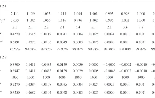
s . Especially for the TABLE 1
PRIORPARAMETERSANDESTIMATESOFSTRUCTURALPARAMETERSFORBOTHMODELS. THECREDIBILITYWEIGHTSARECALCULATEDW.R.T. cj2
AP M [ AND j 2 sYMAP, RESPECTIVELY. j 0 1 2 3 4 5 6 7 8 9 Model 2.1 fj 2.111 1.129 1.033 1.013 1.004 1.001 0.993 0.998 1.000 0.999 jMAP (qX )-1 3.053 1.182 1.056 1.016 0.996 1.002 0.996 1.002 1.000 1.001 gj 2.1 2.1 2.2 2.1 3.4 2.1 2.1 3.4 7.7 7.5 j c[2MAP 0.4270 0.0515 0.0119 0.0041 0.0004 0.0025 0.0024 0.0001 0.0001 0.0002 j hoc -c2ad [ 0.6891 0.0773 0.0106 0.0049 0.0003 0.0025 0.0020 0.0001 0.0001 0.0002 aj, 0 97.59% 99.69% 99.92% 99.97% 99.99% 99.98% 99.98% 100.00% 99.99% 99.99% Model 2.2 zj 0.8900 0.1411 0.0483 0.0139 0.0030 0.0005 – 0.0005 – 0.0002 – 0.0010 – 0.0006 j AP mM Y 0.8947 0.1411 0.0483 0.0139 0.0029 0.0005 – 0.0048 – 0.0002 – 0.0010 – 0.0006 nj 1000 1000 1000 1000 1000 1000 1000 1000 1000 1000 j s2MAP Y 0.2270 0.0384 0.0108 0.0035 0.0004 0.0024 0.0025 0.0001 0.0001 0.0002 hoc j -s2ad Y 0.3250 0.0682 0.0104 0.0048 0.0003 0.0025 0.0020 0.0001 0.0001 0.0002 rj, 0 100.00% 100.00% 100.00% 100.00% 100.00% 100.00% 100.00% 100.00% 100.00% 100.00%
most recent accident years i = 19,20, we observe that higher values of j hoc -c[2ad and j hoc -2 sYad , compared to cj2 AP M [ and j , 2
sYMAP lead to higher skewness and excess kurtosis. As mentioned in Section 2, Model 2.1 involves the inverse gamma distribution which may lead to heavy-tailed distributions for the CDR given DI and higher moments thereof may fail to exist. In fact for this example we
observe that the minimum order (over all accident years and BU’s) up to which moments exist is n = 48 w.r.t. MAP estimators and n = 31 w.r.t. ad-hoc estima-tors. On the other hand we point out that for Model 2.2 all moments exist.
5.2. Aggregated Accident Years
In the following we consider the results for aggregated accident years. We calcu-late higher moments according to Theorem 3.8 and derive the values for the skewness and the excess kurtosis. To highlight the infl uence of the considera-tion of skewness and excess kurtosis in the uncertainty analysis of the CDR we then fi t a distribution from the 4-parameter Johnson family of distributions (see Johnson et al. [11]), which includes the shifted lognormal distribution as a special case, to the fi rst four moments of the CDR and compare the results for the standard shifted lognormal fi t taking only the fi rst two moments into account as proposed in Solvency II. The Johnson fi t can either be calculated by the help of tables (see Johnson [10]) or by iterative methods as described in Elderton-Johnson [4]. For this case study we made use of the function JohnsonFit implemented in the R-package SuppDists for which a fi t by moments, presented in Hill et al. [8], is applied. In the following we restrict our consideration to results w.r.t. MAP estimators which are more robust com-pared to ad-hoc estimators.
From Table 2 we observe skewness to the right and positive excess kurtosis in all cases. The distribution fi t resulting from JohnsonFit lies in the so-called SU-system represented by 1 -, sinh Z=g+d 'X-l z1
where Z has standard normal distribution, for more details see Johnson et al. [11]. As documented in the help fi le of the R-package SuppDists fi tting by moments is diffi cult and the function JohnsonFit may report an error in some cases which happens for BUA (see Table 2) in our example. For the other
BU’s we see that the fi tted Johnson distributions fi t the skewness and excess kurtosis very close whereas the values for the fi tted shifted lognormal distribu-tions signifi cantly deviate. Note that the shifted lognormal fi t currently used in insurance industry provides substantially lower skewness and excess kurto-sis. As a representative for all BU’s Figure 3 illustrates the fi tted densities for BUC for Model 2.1 and Model 2.2.
In summary, we calculate exact moments for Model 2.1 and Model 2.2. For these moments we then fi t the standard shifted lognormal distribution to the
fi rst two moments as proposed in Solvency II. Comparing this approximation to the 4-parameter Johnson approximation, using the exact skewness and excess kurtosis resulting from Model 2.1 and Model 2.2 respectively, shows that the approximation for the standard shifted lognormal distribution is too symmetric and fails to fi t the skewness and the excess kurtosis of the distribution of the CDR (see Table 2). This has signifi cant infl uence in setting confi -dence levels or choosing risk adjustment estimation techniques as discussed in IASB [9]: Figure 4 shows quantiles for the Johnson and the shifted lognormal approximation as a function of the confi dence level for both models w.r.t. BUC. For both models the quantiles of the Johnson fi t are smaller than the
quantiles of the shifted lognormal approximation for confi dence levels below 90%. Slightly above the 90% confi dence level they become equal and then start to signifi cantly deviate (values up to confi dence level 99.5% used in Solvency II are provided), where the quantiles of the Johnson fi t are larger compared to the quantiles of the shifted lognormal approximation.
TABLE 2
SKEWNESS (S) ANDEXCESSKURTOSIS (EK) OFTHEAGGREGATED CDR W.R.T. THEOREM 3.8 FORTHEFITTED JOHNSONDISTRIBUTION (J) ANDFORTHEFITTEDSHIFTEDLOGNORMAL
DISTRIBUTION (LN) W.R.T. MAP ESTIMATORS.
Model 2.1 Model 2.2 S SJ SLN EK EKJ EKLN S SJ SLN EK EKJ EKLN BUA 1.36 NA 0.23 3.08 NA 0.09 1.56 1.57 0.18 4.92 4.93 0.06 BUB 0.79 0.79 0.10 1.42 1.41 0.02 0.80 0.81 0.09 1.88 1.90 0.01 BUC 1.01 1.01 0.13 2.01 2.00 0.03 1.12 1.11 0.11 3.03 3.01 0.02 BUD 0.89 0.89 0.10 1.68 1.68 0.02 0.96 0.97 0.09 2.43 2.44 0.01 BUE 0.75 0.75 0.12 1.22 1.22 0.02 0.82 0.83 0.10 1.78 1.81 0.02 BUF 0.74 0.74 0.11 1.30 1.30 0.02 0.31 0.32 0.08 0.40 0.41 0.01
FIGURE 3: Fitted densities for the Johnson family of distributions (solid line) and the shifted lognormal distribution (dashed line) for Model 2.1 and Model 2.2 w.r.t. BUC and MAP estimators.
FIGURE 4: Quantiles for the Johnson fi t (solid line) and quantiles for the shifted lognormal distribution (dashed line) as a function of the confi dence level w.r.t. BUC and MAP estimators. Residuals of quantiles
for the two approximations.
As an example we think of two insurers (Insurer A and B) assessing the uncer-tainty of the CDR for BUC. Insurer A calculates moments up to order four
(e.g. calculated w.r.t. Model 2.1) and considers the Johnson fi t and Insurer B calculates the fi rst two moments (w.r.t. Model 2.1) and considers the shifted lognormal fi t. If both choose a quantile slightly on the 90% confi dence level as risk measure they will report about equal risk adjustments. We know that the two approximations result in different values for skewness and excess kur-tosis. This means that in our example the requirement of paragraph B94 in IASB [9] that risk adjustments have to be larger for probability distributions that are more skewed would be violated. Insurer A that calculated moments up to order four knows that the distribution of the CDR is rather skewed and according to paragraph B95 in IASB [9] he concludes that the confi dence level technique is not appropriate and considers other techniques, e.g. the conditional tail expectation, to estimate the risk adjustment. On the other hand Insurer B that considers the shifted lognormal fi t may wrongly account the confi dence level technique to be viable. Therefore, taking factors such as the shape of the distribution into account signifi cantly infl uences the assessment of the uncer-tainty of the CDR as discussed in IASB [9].
Considering high quantiles for the two approximations, e.g. the VaR at the 99.5% confi dence level listed in Table 3, shows that the VaR for the shifted log-normal distribution is signifi cantly lower compared to the VaR for the Johnson
fi t in all cases. However, the fi rst four moments do not tell much about the tail behavior of the distribution of the CDR. Therefore a comprehensive assess-ment of the risk in the tails should take into account techniques from extreme value theory as e.g. presented in Embrechts et al. [5].
Furthermore, we see that the VaR at the 99.5% confi dence level for Model 2.1 is signifi cantly higher than for Model 2.2 for all BU’s. This can partly be explained by the fact that Model 2.1 involves inverse gamma distributions leading to heavy tailed distributions for the CDR for which higher moments fail to exist whereas Model 2.2 results in moderately heavy tailed distributions for which all moments exist.
Remarks.
• Another approach to estimate the VaR taking moments up to order four into account, is provided by the Cornish-Fisher expansion, see e.g. Hill-Davis [7]. In contrast to the Johnson transformation this approach does not rely on distributional assumptions.
• Note that fi rst moments (from which we can calculate the reserves) w.r.t. Model 2.2 are rather sensitive on the structural parameters sj (c.f. (3.8))
whereas for Model 2.1 deviations in the estimation of cj have only marginal
infl uence (via posterior parameters, see Proposition 3.1 and (3.1)). Therefore we conclude that Model 2.1 is more stable for prediction.
• As an extension to the presented 4-parameter approximation within the Johnson family of distributions one could implement non-parametric approx-imations such as Edgeworth expansions or saddlepoint approxapprox-imations based on higher moments. An essential assumption to apply such techniques is the existence of higher moments which is the case for Model 2.2 but for Model 2.1 higher moments may fail to exist. For an overview on this topic we refer to Butler [3].
TABLE 3
VAR AT 99.5% CONFIDENCELEVELANDRESERVESFOR MODEL 2.1 AND MODEL 2.2 W.R.T. MAP ESTIMATORS, FORTHEFITTED JOHNSONDISTRIBUTION (J) ANDTHEFITTED
SHIFTEDLOGNORMALDISTRIBUTION (LN).
Model 2.1 Model 2.2
VaRJ VaRLN reserves VaRJ VaRLN reserves BUA NA 2110 815 2429 1668 847 BUB 1075 849 321 963 741 372 BUC 1942 1473 748 1776 1289 852 BUD 3846 2962 1498 3517 2610 1708 BUE 2081 1674 570 1914 1479 716 BUF 208 167 114 123 111 77
CONCLUSION
We have studied the claims development result (CDR). The CDR is one of the major risk drivers in the profi t and loss statement of a general insurance com-pany and therefore needs a careful and appropriate risk assessment. In addi-tion to the existing actuarial literature we determine higher order moments of the CDR distribution (for two different analytical models). The consideration of higher moments allows insurance companies to gain more insight into the shape of the distribution of the CDR, by e.g. considering the skewness and the excess kurtosis, which is essential for the application of techniques for estimating risk adjustments of future cash fl ows as discussed in IASB [9].
As proposed in Solvency II and applied in current practice, a proxy for the distribution of the CDR is obtained by fi tting a shifted lognormal distribution to the estimates of the fi rst two moments of the CDR. Within the 4-parameter Johnson family of distributions we refi ne the approximation for higher moments by including skewness and excess kurtosis parameters. The case study shows that the shifted lognormal approximation may result in too symmetric distri-butions which fail to fi t the skewness and the excess kurtosis of the distribu-tion of the CDR. Taking factors such as the shape of the distribudistribu-tion into account signifi cantly infl uences the estimation of risk adjustments as discussed in IASB [9] and therefore knowledge about higher moments of the CDR con-tributes to a comprehensive assessment of the reserving risk.
REFERENCES
[1] BÜHLMANN, H., DE FELICE, M., GISLER, A., MORICONI, F. and WÜTHRICH, M.V. (2009) Recursive credibility formula for chain ladder factors and the claims development result.
ASTIN Bulletin, 39(1), 275-306.
[2] BÜHLMANN, H. and GISLER, A. (2005) A Course in Credibility Theory and its Applications.
Springer.
[3] BUTLER, R.W. (2007) Saddlepoint Approximations with Applications. Cambridge University Press.
[4] ELDERTON, W.P. and JOHNSON, N.L. (1969) System of Frequency Curves. Cambridge Uni-versity Press.
[5] EMBRECHTS, P., KLÜPPELBERG, C. and MIKOSCH, T. (1997) Modelling Extremal Events for
Insurance and Finance. Springer.
[6] GISLER, A. and WÜTHRICH, M.V. (2008) Credibility for the chain ladder reserving method.
ASTIN Bulletin, 38(2), 565-600.
[7] HILL, G.W. and DAVIS, A.W. (1968) Generalized asymptotic expansions of Cornish-Fisher
type. The Annals of Mathematical Statistics, 39(4), 1264-1273.
[8] HILL, I.D., HILL, R. and HOLDER, R.L. (1976) Fitting Johnson curves by moments. Applied
Statistics, 25(2), 180-189.
[9] IASB (2010) Exposure Draft Insurance Contracts. ED/2010/8, available under http://www. ifrs.org
[10] JOHNSON, N.L. (1965) Tables to facilitate fi tting Su frequency curves. Biometrika, 52(3/4), 547-558.
[11] JOHNSON, N.L., KOTZ, S. and BALAKRISHNAN, N. (1994) Continuous Univariate Distributions
(Volume 1, 2nd Edition). Wiley series in probability and mathematical statistics.
[12] MACK, T. (1993) Distribution-free calculation of the standard error of chain ladder reserve estimates. ASTIN Bulletin, 23(2), 213-225.
[13] MACK, T. (1994) Measuring the variability of chain ladder reserve estimates. Casualty
Actu-arial Society Forum 1, Spring 1994, 101-182.
[14] MCNEIL, A.J., FREY, R. and EMBRECHTS, P. (2005) Quantitative Risk Management: Concepts,
Techniques and Tools. Princeton University Press.
[15] SALZMANN, R. and WÜTHRICH, M.V. (2010) Cost-of-capital margin for a general insurance liability runoff. ASTIN Bulletin, 40(2), 415-451.
[16] WÜTHRICH, M.V. and MERZ, M. (2008) Stochastic Claims Reserving Methods in Insurance. Wiley Finance. ROBERT SALZMANN ETH Zurich RiskLab Switzerland Department of Mathematics 8092 Zurich Switzerland MARIO V. WÜTHRICH ETH Zurich RiskLab Switzerland Department of Mathematics 8092 Zurich Switzerland MICHAEL MERZ University of Hamburg
Department of Business Administration 20146 Hamburg
A. APPENDIX
Proof of Proposition 3.1. We start with proving the result for Model 2.1.
(a) We denote the distribution of Ci, 0 by pi. By the chain rule of conditional
probability and the Markov assumption in Model 2.1 the joint density of (Q, DI + t) is given by j j j j j j j j j j -j , j Q 1 2 2 -2 2 2 ( ) ( 1) 1) ( ) . exp exp g F F f f C D D , 1 , , I t I t i j I t i j i j j j J j j i i I i 1 1 0 1 0 0 j # c c c p
q
G G = -- -# c + + -+ + -= -= p g q q q ( g c g -g g _ a a ^ a ^ ` ` i k k h k h j j%
%
%
Note that g (DI + t – 1) is some norming function depending on terms Ci, j !
DI + t – 1. This implies that the posterior density of Q, given DI + t, satisfi es
the following proportionality property
j j j j -2 1 g + -|DI t exp F, ( 1) . I j t j J i j i I j t j j 0 1 0 1 j ? q c Q c - + -+ - + = -= - - + p_ i
%
2 f q f/
f g ppThese are independent gamma densities which proves the claim for Model 2.1. (b) Similar as above for Model 2.2, the joint density of ( m, DI + t) is given as
follows: j j j j j i 2 2 , ( ) ( ) ( ) ( ) . exp exp g F C D D ( ) , log I t I t i F i j I t j J i I i 1 2 1 0 1 2 0 0 , i j 2 p = # s n z + + -- -+ + - = -= m s p p 2 -p , j 2 m n j mj 2 ^ h ^ h ^ h
%
%
%
This implies that the posterior density of m, given DI + t, satisfi es the
fol-lowing proportionality property
, j t D 2 | I t exp , , j J j j t 0 1 2 2 ? n -+ = -p^m h
%
f ^m -z h p with j j j j j t + -i=0 1 ( ) ( log j F , , j t i j z = + - + n s 2 2 I- - +j 1 t I 2 2 n s ) , z/
and j , j j j t t -1 ( j ) . 2 n = + - + n s n 2 I 2 2These are independent normal densities which proves the claim for Model 2.2. ¡
Proof of Proposition 3.6. Let us fi rst prove the result for Model 2.1. (a) Due to Proposition 3.1 and Corollary 3.3 we fi nd for n ! N that
j , i J j j C Ci I, i FI j j, (1 )F . j I i J n 1 1 1 = - + - + -= - + -b b ) n ) 1 n 0 ( ( ` j ^ h
%
a kWith the binomial formula, this rewrites as
j , iJ j l j C C n 1 F . l F , , n i I i l n j I i J I j j l 1 0 1 1 = - + -= = - + -) ( ) b n-l ) 1 n 0 ( b ( n-l ` j ^ h
%
/
f p ^ h^ h ` jWith this, we get
j , i l J . j j C F (C ) n l F 1 E E D , , n I i I i n l n j I i J I j j l I 1 0 1 1 = - + -= = - + -( ) n-l ) ) b D 1 0 ( n-l ( b ` f ^ ^ ` j p h h j 9 > C H
%
/
Due to posterior independence the above expression on the right can be written as follows: j l j j F . C F n l F 1 E E D , , , i I i i I i I l n j I i J I j j l I 0 1 1 -- -= = - + -- b n n n-l ) D ( )b (0 n-l ^ h 6^ h @
%
/
f p 9^ h C^ h ^ hNow we consider terms of the form
j ,
F
E9^ I-j, hk DIC
for 0 < k # n and j = I – i, …, J – 1. By the assumptions of Model 2.1, the tower property for conditional expectations and Proposition 3.1 we get
j j j j j j j , j + -, j 0 2 2 2 2 k , . F F k c k k E , D E E , D D E D , I j j k I I j j k I I k I j 0 0 c c c c c c Q G G G G G G = = + = -- -q g 2 2 k g ^ ^ a a a a a a ^ ^ h h k k k k k k h h 9 C
6
6
@
@
9 CThe above expression is obtained by applying twice formula (2.1) for the moments of a gamma distributed random variable. Since the last expression corresponds to Kk, j, this proves the proposition for Model 2.1.
(b) First we note that (c.f. (3.10)) j , iJ j , j 1 C C exp exp Y . 2 , i I i j I i J n 1 1 1 2 2 = - + = - + - s n ) + ) n 1 ( (1 ^ h f
%
c m ^ hp Hence we get j j , i , j J 1 C C exp exp Y . 2 E n DI E i I, i D j I i J n I 1 1 1 2 2 = - + = - + - s n ) ) + 1 1 ( ( ^ h f c m ^ hp 9 C >%
HDue to posterior independence the above expression on the right can be written as follows: j j, j n n 1 Y (C ) F exp n n . 2 E D E D , , i I i i I i I j I i J I 1 1 2+ - -= - + - s n exp 2 ) 1 ( ^ h e o a k
6
@
%
9 CBy the assumptions of Model 2.2 and Proposition 3.1 we obtain
0 n n , I i I i I i -- -E E E , E . exp exp exp F F n n n 2 2 2 D D D , , , i I i n I i I i n I I I i I I i 2 2 2 2 0 2 2 D m m n = = + = + - - -s s z ^ ^ c c c h h m m m
6
@
6
6
@
@
; EFurthermore we have that (see Corollary 3.5)
Y j j j j D Y Y E exp n DI = exp n(1-k) E n I-j j, I . ) ) exp k 1 0 ( ( a k a k ^ h 9 C
6
@
Since YI – j, j, for given m and DI, are normally distributed with N(mj, sj) and
using Proposition 3.1 we fi nd Y Y j j j 0, , D , j 0 m j j j j j j j j D s s ( ( ( E E E E ) ) ) . exp exp exp exp exp n n n n n n n 2 2 2 D , , I j I I j I I I 2 2 2 2 2 2 z = = + + - -m n D = k k k k k k k j j ^ ^ e c c h h o m m
6
9 8>
@
B CH
Rearranging the terms accordingly completes the proof.
Proof of Proposition 3.7. For i = I – J + 1 we have that Ci J,(1) = Ci, I – i + 1. By the
assumptions of Model 2.2 we fi nd in this case that
, i J L I-i C N log C( ) , , ,C i I, i I i 2 , i + + m - - s ) m 1 ( I-i ^ h
By formula (2.4) and Proposition 3.1 we obtain for Ci J(,1) and i > I – j + 1
j j j j j j j j j , i exp J , , j j 1 1 2 2 2 -- j j k=0 C E E ( ) ( ) . exp exp log exp
exp exp log
exp C C C I j F F j F C 2 1 1 2 2 1 1 2 2 D D , , , , , , , i J I i I i j I i J I i I i j I i J j I j k j i I i j I i J j k I j k j i I i 1 1 1 1 1 2 1 1 1 2 2 1 1 2 2 1 1 2 0 2 2 # n z n n = = = + - + + + = + - + + + -= - + -+ -= - + - - - + -= - + -= -s s s s n s s n ) + + m 1 I k ( z ^ c ^
f
e f f ^ c h m hp
o p hp m 6 8 @ B%
%
%
/
/
By collecting DI-measurable terms in bj , i.e. ,
j j j j 1, 2 -j j j 1 ( 1) ,
exp log F exp exp
j 2 2 , k I j k j 0 1 2 2 2 n = + - + + = -s s n I k z b f
/
^ hpf
p
e o we get , i J j C Fi, exp log F , C, . j I i J I j j i j 1 1 = = - + -) I-i 1 I-i k ( b ` a jk%
We write i k j , i J jlog C exp log Fi I, i F , C, b . j I i J I j j i I i j I i J d 1 1 1 1 = -= - + -- -= - + -= ) ⬘ 1 ( + ^ ^ f h hp 14 4 4424 4 443%
/
Using the assumptions of Model 2.2 we obtain that
N kjlog + kjmj, j j . log Fi I i F , j I i J I j j j I i J j I i J 1 1 1 2 1 2 I k = = = -s + , , mD + ^ h