Deterministic approach to polarization mode dispersion

Deterministic Approach to Polarization Mode

Dispersion

by

Poh-Boon Phua

Submitted to the Department of Electrical Engineering and Computer

Science

in partial fulfillment of the requirements for the degree of

Doctor of Philosophy

at the

MASSACHUSETTS INSTITUTE OF TECHNOLOGY

August 2004

c

° Massachusetts Institute of Technology 2004. All rights reserved.

Author . . . .

Poh-Boon Phua

Department of Electrical Engineering and Computer Science

August 18, 2004

Certified by . . . .

Erich P. Ippen

Elihu Thomson Professor of Electrical Engineering, Professor of

Physics

Thesis Supervisor

Accepted by . . . .

Arthur C. Smith

Chairman, Department Committee on Graduate Students

Deterministic Approach to Polarization Mode Dispersion

by

Poh-Boon Phua

Submitted to the Department of Electrical Engineering and Computer Science on August 18, 2004, in partial fulfillment of the

requirements for the degree of Doctor of Philosophy

Abstract

Polarization Mode Dispersion (PMD) is considered to be one of the most serious obstacles in the high speed optical telecommunication systems. This thesis focuses on a deterministic approach to both compensation and emulation of PMD. Most PMD compensation schemes in the literature rely on feedback loops to search for the optimum control parameters in the compensator. These schemes often suffer from slow response time and are limited to compensating the low orders of PMD. Adding control parameters to enable higher-order PMD compensation further increases the complexity of the feedback algorithm and its response time. As PMD can vary as fast as on a millisecond time scale, a potential method to alleviate this problem is to employ a deterministic approach to PMD compensation where the PMD parameters are first diagnosed and the compensator then set accordingly.

One of the most challenging problems to this deterministic approach is the real-time monitoring of the PMD information. We propose an improved version of the PMD estimation technique using polarization scrambling and optical filtering. Once the PMD parameters are characterized, for first order PMD compensation, we present a novel module that can produce variable Differential Group Delay (DGD) without any second order PMD. We also discuss a feed-forward PMD compensator for first and second order PMD compensation. To allow for hybrid feed-forward and feedback PMD compensation scheme, we propose to decouple the first and second order PMD compensation by using a module that produces variable second order PMD without any first order PMD. To extend the compensation to all orders of PMD, instead of concatenating birefringent segments, we look into a compensator that is based on four stages of flexible frequency-dependent polarization rotations. These stages can be implemented using polarization beam splitting in combination with spatial light modulators or all-pass filters. For transmission systems where Polarization Dependent Loss (PDL) is an issue, we present a deterministic broadband PDL compensation.

Another important area of research in PMD is its emulation. Traditional PMD emulators are built by cascading a large number of birefringent elements via polariza-tion scramblers. There are two issues with these emulators. Firstly, they are costly and bulky due mainly to the large number of polarization scramblers involved. We

present a combinatorial approach to build polarization scramblers which significantly reduce the number of phase-plates required. Secondly, it is difficult to use such em-ulators to determine the system’s outage probability since we need to explore an extremely large number of possible configurations to obtain a reliable estimate of the outage probability. A deterministic approach to PMD emulation is therefore a better option. The ability to “dial-in” a desired PMD state to an emulator allows one to quickly examine a PMD compensator by investigating only PMD states that are of interest. In this thesis, we present two deterministically controlled PMD emulators. One of them has the dial-in feature for arbitrary set of first and second order PMD while the other can accept arbitrary spectrum of PMD vectors.

Thesis Supervisor: Erich P. Ippen

Acknowledgments

To me, writing the acknowledgement seems to be the most difficult part of the thesis. I worry that I may not do a good job in expressing my gratitude to the late Prof. Haus, Prof. Ippen and all the friends who had helped to make this “journey” a pleasant and fruitful one.

Time flies! The memory of my first arrival at MIT 4 years ago is still so vivid. After so many wonderful opportunities to interact with brilliant individuals whom I will never get to meet in abundance in other parts of the world, now it is time to go. MIT is indeed the focus of the global intellectual power.

When I first came to MIT, I was excited because I knew I would join the group that built the shortest pulse laser in the world and I would be working under the then President of Optical Society of America, Prof. Erich Ippen. I have always held high regards for the Optical Society of America ever since I started my research career in Optics. The opportunity to learn from Prof. Ippen, one of the pioneers and experimentalists who set the world record for the ultra-short pulse, is what attracted me to MIT. Unfortunately, Lady Luck was not on my side, there was no vacancy for the laser projects in Prof. Ippen’s group. The students whom I spoke to in the group, only had praises for Prof. Ippen as a mentor and as a scientist. This positive feedback only strengthens my belief that Prof Ippen is the ideal advisor for me. I was determined to join the group even if it meant I would have to move into a field of optics other than laser research. Finally Prof. Ippen had a vacancy in the PMD project, working closely with Prof Haus.

Looking back, this seems to be a good move because venturing into a new research area in optics every few years, can inject refreshing ideas and new perspectives to the understanding of light. And I believe this is how Prof. Haus acquired a profound insight into so many different areas of optics.

All along I have known that Prof. Haus was a great theorist, the father of the theory of modelocked laser, and was a MIT Institute Professor. But as I started out as an experimentalist for my research career in DSO National Laboratories (Singapore),

I worried that my level of understanding of physics and standard of mathematics may not be up to his expectation. Moreover, PMD is totally a new ball game for me. Nevertheless, my first contact with Prof. Haus was really exciting. Personally, I felt he treated me as if I was already an expert in PMD despite my limited knowledge in polarization. In the meeting, I was overwhelmed by the subtleties of PMD. He “drowned” me with difficult concepts such like Principal State of Polarization and his own analogy of describing the Different Group Velocity as “sausages”. This meeting was daunting as I only managed to understand less than 20 % of what he told me, mostly due to the “impedance mismatch” in our levels of understanding. Fortunately, this “impedance mismatch” decreased as the days passed.

Prof Haus was always so approachable and was always there in his office even though he had retired. His office is beside mine. Most of the times when I passed by his office, I would see him in such intense concentration solving equations at his desk. He liked to solve them on clean sheets of paper which later became his memo with a serial number.

Prof. Haus always impressed me with his deep understanding on almost every-thing. He had an amazingly good memory. He was always able to recall the details of our discussions weeks or months ago which I myself might not have remembered. Another interesting observation was that he took our weekly group presentation more seriously than anyone else. Every presenter in our weekly group meeting seemed to have learnt something from him, or to get their problem solved after the presentation. I always felt that he treated me more like his friend and research collaborator than his student. He had given me many good research directions which had yielded fruitful results. At the same time, he respected my quest to explore my own ideas. Prof Haus was very enthusiastic to pursue a broadband PMD compensation by treating all PMD vectors simply as first order PMD varying with frequency. He encouraged me to look into the details of how to build such compensator. However, at the time, I was busy running simulations on my new idea of handling the low-order PMD. Despite his keen interest in this all-frequency compensation approach, he still gave me full attention in our discussion of my new idea. However, after each discussion, he would often shift

gears trying to explain to me the importance of the all-frequency PMD approach. But one thing he never did, was ask me what I had done on his idea, even though I believed he knew that I had yet to spend more thought on his idea. He persistently sold me this idea for 4 or 5 times. On one occasion, when we took a stroll back after lunch with the one of the invited speakers for the Optics seminar, he told me that he had been thinking over the idea on his bed the night before, and the more he thought of it the more feasible he felt it was. At this point, I really felt bad that I did not do much on this idea yet even after his many persuasions. The saddest thing was it happened to be one of our last discussions on this topic before his sudden departure a few weeks later. I worked on this idea right after his funeral. With much difficulty, I finally managed to come out with the architecture of such an All-Frequency PMD compensator. I am not sure whether this is what he wanted. Maybe there is a better architecture. Anyway, from simulation, the architecture seems promising and it has given me the better performance than all the other compensators that I have explored. Prof. Haus was a great teacher who had inspired me in many ways especially his pursuit for academic excellence, his passion for science and his enthusiasm in overcoming challenging problems. To me, he was just like the giant “float” which you can always rely on in the sea of knowledge. Prof. Haus had not only inspired me academically, he had also inspired me as someone who had led a fruitful life and enjoyed it to the fullest. He amazed me as a person who dedicated his whole career life to MIT and his private life to a successful marriage that lasted for more than 50 years. It really touches me when Mrs Haus cried out “he’s my life” at the cemetery when she accompanied my family to pay respect to Prof. Haus after my thesis defense. I will always keep Prof. Haus in remembrance and use his teaching as a guide in my future research career.

Prof. Ippen took over my project and I was happy for this increased chances of interaction with him. I am impressed by Prof. Ippen’s ability to explain difficult concepts in a simple manner. Besides his profound technical knowledge and good intuition in optics, I admired him for his charismatic leadership, his sincerity toward people and the warmth he showered. I am always so comfortable with him. From

him, I have learnt how to be a good professor well-liked by his peers and students. While I treasured the freedom he has given me in pursuing the research, he is always there to guide and help. I will also miss Prof Ippen’s sense of humor, sometimes his humorous comments during group meeting just brighten up everyone.

I would also like to thank Prof. Rajeev Ram and Prof. Franz Kartner for their willingness to be in my thesis committee. Their valuable comments have helped to make this thesis a better one. I also like to thank Mike Watts and HanFei Shen for being such wonderful officemates; Milos Popovic and Mike Watts for their helpful discussion in optical filter and waveguides; Peter Rakich, Jason Sicker and Juliet Gopinath for their help in the experiment; Dorothy and Donna for all their help in the administrative issues and many friends in the optics group that have helped me in one way or another. I will definitely miss the Oktoberfest at Prof. Ippen’s house: Mrs Ippen’s cooking and Prof. Ippen’s barbecue cook-out. And of course, Mrs Kartner’s cooking at the Christmas Party held at Prof. Kartner’s house.

Last but not least, I would like to thank my wife Aina and my daughter D’alene. They have given me so much support and family warmth to keep me going. Aina has made me realize that work is not everything, family life is just as important. They are the “de-stressing” tools of my life. I have always believed this helps in my creativity and productivity. They share my ups and downs. I am glad that we have the opportunity to travel quite a bit as a family in US. Aina has always instilled the right attitudes and my outlook in life. She once said ”Simplicity is beauty” which works for me in my research ideas too. Usually simple ideas turn out to be great ideas. Although this acknowledgement is not a love letter, I really hope that Prof. Haus and Mrs Haus have set a good example for our marriage. Mrs Haus had said “it’s a love affair” even after 50 years of marriage to Prof. Haus. So I hope if I “go” before you, you would still say to people “he’s my life”. So, Mrs Dr. Phua, this thesis is dedicated to you and D’alene. D’alene, I hope you will keep and cherish all the good memories of how you spent your early childhood years in US, if you happen to read this many years from now. You are the most beautiful experimental result that I have ever attained.

Getting a PhD has been one of my goals for academic excellence since I was young, I am grateful that DSO had helped me to attain this achievement with its scholarship. I would also like to acknowledge 3M for their funding.

Contents

1 Outline of Thesis 27

2 Polarization Effects in Lightwave System 33

2.1 Background . . . 33

2.2 Origin of PMD . . . 35

2.3 Representations of Polarization and its Evolution . . . 36

2.4 Polarization Controller . . . 43

2.5 Principal State Model . . . 44

2.6 The Law of Infinitesimal Rotation . . . 47

2.7 PMD Concatenation Rule and Dynamical PMD Equation . . . 49

2.8 Higher-Orders PMD . . . 51 2.9 PMD Characterization Technique . . . 54 2.10 Statistics of PMD . . . 56 2.11 System effects of PMD . . . 58 2.12 PMD Mitigation . . . 60 2.13 PMD Compensation . . . 61 2.14 PMD Emulation . . . 64 2.15 PMD in the presence of PDL . . . 65 3 Real-Time PMD Monitoring 67 3.1 Background . . . 67

3.2 Theory of First Order PMD Characterization . . . 68

3.4 Simulations . . . 74

3.5 Broadband PMD Monitoring . . . 79

3.6 Experimental Demonstration . . . 83

3.7 Conclusion . . . 87

4 A Variable DGD Module for First Order PMD 89 4.1 Background . . . 89

4.2 Theory . . . 90

4.3 Simulations . . . 95

4.4 Conclusion . . . 102

5 PMD Compensation Up to Second Order 103 5.1 Background . . . 103

5.2 Theory . . . 104

5.3 Hybrid Feed-forward and Feedback Scheme . . . 110

5.4 Conclusion . . . 118

6 All-Frequency PMD Compensation in Feed-Forward Scheme 120 6.1 Background . . . 120

6.2 Synthesis of Rotation Angle Profiles . . . 122

6.3 Simulations to verify synthesis algorithm . . . 126

6.4 Practical implementations of AFPMD compensator . . . 132

6.5 AFPMD based on All-Pass Filter . . . 133

6.6 Fitting Algorithm for Broadband APF Application . . . 137

6.7 Group delay of APFs, Minimum-Phase Denominator and DGD . . . . 140

6.8 Relationship between Minimum-Phase Response and Cepstral Coeffi-cients . . . 143

6.9 Summary of fitting algorithm . . . 145

6.10 Simulation . . . 146

7 Combinatorial Polarization Scramblers for Many-Segment Emulator150

7.1 Background . . . 150

7.2 Numerical simulation . . . 152

7.3 Experiment . . . 154

7.4 Conclusion . . . 158

8 Deterministic Emulator for First and Second Order PMD 159 8.1 Background . . . 159

8.2 Theory . . . 160

8.3 Simulations & Discussions . . . 167

8.4 Conclusion . . . 174

9 Deterministic Broadband PMD Emulator 175 9.1 Background . . . 175

9.2 Theory . . . 175

9.3 Simulations and Discussions . . . 179

10 Deterministic Broadband PDL Compensator 183 10.1 Background . . . 183

10.2 Synthesis Algorithm . . . 187

10.3 Simulations to verify synthesis algorithm . . . 195

10.4 Practical Implementations . . . 198

10.5 Conclusion . . . 202

List of Figures

2-1 Intrinsic and extrinsic birefringence in optical fiber . . . 35

2-2 Various SOPs in Poincar´e sphere representation . . . 40

2-3 Two typical types of polarization controller . . . 43

2-4 Concatenation of two fiber segments . . . 49

2-5 A long piece of fiber concatenated to a differentially small fiber addition of length ∆z . . . . 50

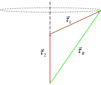
2-6 A vector diagram of the second order PMD and its components . . . 52

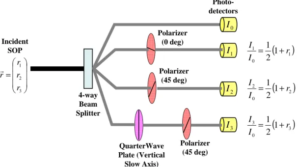
2-7 Schematics of a polarimeter . . . 56

2-8 Maxwellian probability distributions for the DGD and Gaussian dis-tribution for each of the components of the PMD vector . . . 57

3-1 Schematics of the new PMD estimation technique. At the output end of fiber, signal is tapped and filtered. Its averaged SOP is measured using a polarimeter. Various input SOP are generated using a polarization scrambler at the input end of fiber. . . 69

3-2 Optical Spectrum of a 10 Gbit/s RZ pseudo-random bit sequence of length (27_{-1 ). Each ’1’ bit is a Gaussian pulse of 30ps FWHM} pulse-width. . . 70

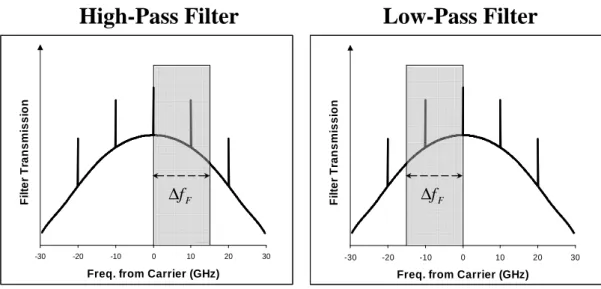
3-3 Transmission profiles of the high-pass filter and low-pass filter used in the PMD estimation techniques . . . 71

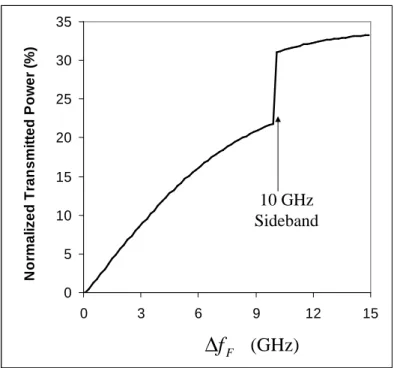
3-4 Normalized average power transmitted by the optical filters for various ∆fF. . . 72

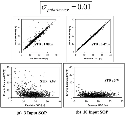
3-5 Graphs in the top row show the estimated DGD versus the emulator’s DGD while the graphs in the bottom row show the errors in the es-timation of the output PSP (in terms of degrees of arc length from the emulator’s output PSP). PMD estimation using various numbers of input SOP: a) 3, b) 5 and c) 10. The standard deviation, σpolarimeter,

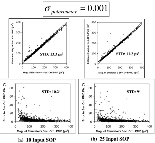
of the polarimetric measurement is kept constant at 0.01. . . 73 3-6 Estimation of the second order PMD using a) 10 and b) 25 input

SOP’s. Standard deviation σpolarimeter used in the simulation is 0.001.

The filter bandwidth ∆fF is 5 GHz. . . 75

3-7 Estimation of first order PMD when Lorentzian filters are used. The low-pass filter has a bandwidth of 3 GHz (FWHM) while the high-pass filter has a bandwidth of 2.5 GHz (FWHM). Both filters are centered 3.5 GHz away from fo. The narrowband filter has a bandwidth of 0.5

GHz (FWHM) centered at fo. Standard deviation σpolarimeter used in

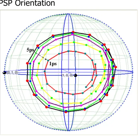
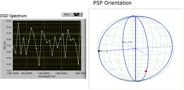
the simulation is 0.01. The number of input SOP’s used are (a) 3 and (b) 10. . . 77 3-8 Measured DGD and PSP as a function of wavelength. The calibrated

emulator’s DGD setting is 5ps . . . 82 3-9 Measured DGD and its errors for the various emulator’s DGD setting 83 3-10 Vector diagram showing the precession of the resultant PMD vector

with wavelength for a two-segment concatenation . . . 84 3-11 The measured PSP and DGD as a function of wavelength for a

two-segment concatenation . . . 85 3-12 Measured resultant PSP as a function of wavelength for different

set-ting of the first segment’s DGD . . . 86 3-13 Deduced DGD of the individual segment . . . 87 4-1 Schematic of the variable DGD module. It consists of two identical

blocks concatenated via C1. Each block itself consists of two identical

4-2 Construction of ~τ 0 and ~τ_ω0 in Stokes space. Step 1 is the C0

transfor-mation of ~τ, which correspond to a rotation of θC0 about y-axis. Step

2 is the R transformation of C0~τ which corresponds to a rotation of θR

about x-axis. In Step 3, vector addition of ~τ and RC0~τ gives ~τ

0

while vector product ~τ of and RC0~τ give ~τ

0

ω. . . 91

4-3 ~τ 0 and ~τ_ω0 under RBC1(= RC0RC1) transformation in Stokes space.

Point (1) to Point (2): ~τ 0 and ~τ_ω0 are transformed by C1 which

cor-responds to a rotation of θC1 about x-axis. Point (2) to Point (3):

R transformation which corresponds to a rotation of θR about x-axis.

Point (3) to Point (4): C0 transformation which corresponds to a

ro-tation of θC0 about y-axis. Point (4) back to Point (1): another R

transformation. . . 93 4-4 DGD produced by the 4-segment module for various designated DGD

values. . . 94 4-5 Higher-orders PMD produced the 4-segment module. (a) Magnitude of

second order PMD vector. (b) Magnitude of third order PMD vector. For comparison purposes, we have also plotted higher-orders PMD pro-duced by the conventional concatenation of two 25 ps DGD segments via a polarization controller, to produce the same DGD tuning range of 50 ps. . . 95 4-6 (a) Numerical solutions of rotation angle of C0 for various designated

DGD values using equation (4.9). (b) Numerical solution of rotation angle of C1 for three different cases: case (1): Rotation angle of all

segments are equal to 2.23 rad; case (2): -2.8 rad (first segment), -1.7 rad (second segment), 3.3 rad (third segment), 5.1 rad (fourth seg-ment); case (3): 4.5 rad (first segment), 2.5 rad (second segment), -3.5 rad (third segment), 1.5 rad (fourth segment). Solutions are computed using equation (4.10). . . 97

4-7 First and second order PMD generated for various angle standard devi-ation σangleof (a) 0.01o, (b) 0.1o and (c) 1o. All segments have identical

|~τ| of 12.5ps and R. . . . 98

4-8 a) DGD and b) Magnitude of second order PMD vary periodically when the optical frequency is shifted from the center frequency. Four different DGD values (at the center frequency) are shown: 5 ps, 10 ps, 15 ps and 19 ps. Each segment in the module has DGD of 5 ps and the total DGD tuning range is 20 ps. . . 100 4-9 a) 4-segment module used in first order PMD compensation; b)

Con-ventional 2-segment concatenation used in first order PMD compensa-tion. Due to the 15ps DGD presented in the first order emulator, the pulses after emulator are distorted (shown as the bottom dark solid line). The upper light solid line is the input pulse-shape. Triangles are for the case of positive 245 GHz/ns frequency chirp, circles are for the case of negative 245 GHz/ns frequency chirp while crosses are for the case of zero frequency chirp. For 4-segment module, full restora-tion of the pulse is observed regardless of the frequency chirp while chirp-dependent distortion is observed for the conventional 2-segment concatenation. . . 101 5-1 The three-segment compensator consisting of three first order PMD

segments and two polarization rotators. The first segment is of ad-justable DGD. ~τf and ~τωf are the first and second order PMD of

trans-mission cable while ~τcand ~τωcare those of the compensator. For PMD

compensation, we need to set C0 and the compensator appropriately

5-2 (a) Relative orientations of ~τc, ~τωc, ~τ3, ~A and ~B. φ is the angle between

~τc and ~τωc which is required to be the same as that between ~τf and ~τωf.

Condition (5.11) requires ~τωc to be perpendicular to ~τc− ~τ3. C0 allows

us to arbitrarily fix ~τc and ~τωc on any arbitrary plane that contains ~τ3. Vectors ~A and − ~B point from centre of spheres to a point on the

ring of intersection of the two spheres so as to satisfy equation (5.9) and (5.10) simultaneously. (b) The cross product of ~B and ~τc − ~τ3

gives ~τωc − (~τ3 × ~τc). Vector ˆq is the unit vector in the direction of

[(~τc− ~τ3) × (~τωc− (~τ3× ~τc)] while ˆp is the unit vector in the direction

of (~τc− ~τ3). . . 108

5-3 Block diagram of two PMD blocks concatenated via polarization con-troller. . . 110 5-4 Schematic of our proposed module that produces variable magnitude

of second order PMD without first order PMD. It consists of 4 identical fixed DGD segments arranged in a symmetrical manner. The first and second fixed DGD segments of PMD ~τ are concatenated via Coto form

the Block 1 while Block 2 is formed by the third and fourth segment of PMD −~τ, concatenated using another Co. The polarization controller C between the two blocks is made up of two fixed phase plates and one

tunable phase-plate C†

o. . . 112

5-5 (a) Magnitudes of second order PMD produced by our module for var-ious designated magnitude values. (b) Magnitude of third order PMD vector produced by our module when it is controlled to produce the designated magnitude of second order PMD. For comparison purposes, we have also plotted the third order PMD produced by our previous 3-segments configuration (see Ref. [1]) for the same tuning range of 312.5 ps2_{. . . 114}

5-6 First and second order PMD generated by our module when there are angle standard deviations σangle of (a) 0.1o, (b) 0.25o and (c) 0.5o in

the rotation angles of the phase-plates together, with DGD standard deviation σDGD of 0.06ps for all the DGD segments. All segments have

identical |~τ| of 12.5ps. . . 116 6-1 a) Schematic of our 4-stage all-frequency PMD compensator; b) PMD

spectra after fiber, and composite PMD spectra after Stage 2 and 3 of compensator. . . 122 6-2 Required rotation angles of various stages for a randomly chosen fiber:

(a) θ1(ω) of Stage 1 (b) θ2(ω) of Stage 2, (c) θ3(ω) of Stage 3. Solid

curves are exact rotation angles computed using the synthesis algo-rithm while dashed curves are rotation angles approximated using APFs. fo is the carrier’s optical frequency. (d) shows the output

optical signal before and after compensation. Thin solid curve is the input signal to fiber. Thick solid curve is output from fiber. Curve of unfilled triangles is after compensation using the exact rotation an-gles while the curve of filled circles is based on approximated rotation angles using APFs. . . 127 6-3 Cumulative Probability distribution of exceeding a certain BER value.

Dashed curve is the uncompensated case. Performances of compen-sation using different ∆f for the synthesis algorithm are investigated: Solid line curve is for ∆f = 0.63 GHz, curve of squares is for ∆f = 2.54 GHz and curve of crosses is for ∆f = 6.3 GHz. . . . 128 6-4 Performance of compensation when there are monitoring errors in the

spectrum of PMD vectors. Curve of squares is for the case with error variance σP M D = 10ps. For reference, the compensated case without

error is shown as the solid curve. The numerical simulation was carried out with ∆f = 0.63 GHz, and the mean DGD was 20ps for the fiber ensemble. . . 129

6-5 Cumulative probability distribution of BER curve for multi-channel PMD compensation over 1 Tera-Hertz bandwidth. The center wave-length of the 40 Gbit/s Gaussian pulse was randomly chosen within this 1 THz bandwidth. The numerical simulation was carried out with ∆f = 0.63 GHz, and the mean DGD was 20ps for the fiber ensemble. The solid line curve is for the compensated case while the dashed curve is for the uncompensated case. . . 130 6-6 Implementation of PMD compensator using spatial arrays of liquid

crystal polarization rotators with dispersive grating elements. . . 131 6-7 A possible implementation of Figure 1a using All-Pass filters integrated

on planar waveguides. . . 132 6-8 Cumulative probability distribution of BER curve when APFs are

used to approximate the rotation angles calculated by the synthesis algorithm. The curve of crosses is for the compensated case using

N1 = N2 = N3 = 3 APFs, the curve of square is for the compensated

case using N1 = 15, N2 = 10, and N3 = 15 APFs, the solid line curve is

for the compensated case using the exact rotation angles computed by the synthesis algorithm and the dashed curve is for the uncompensated case. The numerical simulation was carried out with ∆f = 1.26 GHz, and the mean DGD was 11.5 ps for the fiber ensemble. . . 135 6-9 A common building block in the broadband PMD compensator . . . . 138 6-10 A random sample of the rotation angle profile θ(ω) required for one of

the frequency dependent polarization rotators used in the broadband PMD compensator. The desired rotation angle profile of θ(ω) is shown by the solid curve while the profile approximated by the APFs is shown by the dashed-curve. The number of APFs used for each polarization arms is 10 for (a), 20 for (b) and 30 for (c). . . 147 6-11 The cumulative probability distribution of the Bit Error Rate (BER)

7-1 Simulated statistics of 100,000 random fiber realizations using the com-binatorial polarization scramblers. Circles show the simulated distri-butions of (a) one of the components of the PMD vector, (b) the DGD, (c) magnitude of second order PMD. The number of bins used is 400. (d) shows the normalized frequency autocorrelation function. The cor-responding theoretical curves are shown in solid line curves. The mean DGD used for fitting these theoretical curves is 4.9 ps. . . 153 7-2 Top: Schematic of an all-fiber PMD emulator using combinatorial

po-larization scramblers. After each PM fiber loop, a different popo-larization scrambler is built by passing different sequence of the 6 fiber squeezers which are labelled letter ”A” to ”F”; Bottom: A photograph of such emulator . . . 154 7-3 (a) Variation and distribution of DGD with fiber realizations at fixed

wavelength; (b) Variation and distribution of DGD with wavelength for fixed fiber realizations . . . 156 7-4 Measured statistics of the all-fiber PMD emulator using the

combinato-rial polarization scramblers. The sample size is 35000 and the number of bins used is 300. Circles show the simulated distributions of a) one of the component of the PMD vector, b) the DGD, c) the magnitude of second order PMD. Figure 3d) shows the measured frequency auto-correlation function in cricles. All the corresponding theoretical curves are shown in solid line curves. The mean DGD used for fitting these theoretical curves is 5ps. . . 157 8-1 Schematics of 4-segment emulator. Segment 1, 2, and 3 have fixed

DGD while Segment 0 has variable DGD. . . 160 8-2 Sequences of combining segments for PMD analysis . . . 163

8-3 (a) Vector ~D is fixed to lie in the plane of (~τ − ~τ3) and (~τω− (~τ3× ~τ)).

It has fixed magnitude of |~τ2| and is in the direction such that (~τ −

~τ3 − ~D)) is perpendicular to (~τω − (~τ3 × ~τ)). (b) Vector ~B has fixed

magnitude of |~τ1| and, once ~D is solved, ~B lies in the orientation such

that ~B × (~τ − ~τ3− ~D) equals to (~τω− (~τ3× ~τ) − ~D × (~τ − ~τ3)). . . . 164

8-4 Monte Carlo simulation of 1st and 2nd order PMD generated by a con-catenation of 100 1-ps DGD segments. (a) Probability density function (pdf) of DGD, |~τ|; (b) pdf of vector components, ~τi , of ~τ. The pdf are

identical for all the 3 vector components; (c) pdf of |~τω|; and (d) pdf of

vector components, ~τωi, of ~τω. Dots are simulation results while solid

lines are the fitting curves. . . 165 8-5 Monte Carlo simulation of 1st and 2nd order PMD generated by a

con-catenation of 4-DGD segments with polarization scramblers between them. The DGD values are 76.3 ps for segment 1, 73.5 ps for segment 2, 2.5 ps for segment 3 while the DGD for segment 0 is randomly chosen from 0 ps to 50 ps. . . 167 8-6 Monte Carlo simulation of 1st and 2nd order PMD generated by the

same concatenation of 4-DGD segments used in Figure 8-5. However, here, the polarization rotators and DGD value of Segment 0 are con-trolled deterministically to produce the realistic pdf in Figure 8-4. (a) Probability density function (pdf) of DGD, |~τ|; (b) pdf of vector com-ponents, ~τi, of ~τ. (c) pdf of |~τω|; and (d) pdf of vector components, ~τωi,

of ~τω. . . 168

8-7 Probability density function (pdf) of the 3rd _{order PMD magnitude,}

|~τωω| generated by 4-segments emulator when generating the 1st and

2nd_{order PMD shown in Figure 8-6. For comparison purposes, we also}

plotted the 3rd _{order PMD pdf generated by the concatenation of 100}

1-ps segments when generating the 1st _{and 2}nd _{order PMD shown in}

8-8 1st and 2nd order PMD probability density functions generated by 4-segments emulator using fixed phase-plates polarization rotators when there is a random Gaussian distributed angular error of standard de-viation σangle in the rotation of the birefringence axes. (a) σangle = 0.3

arc min degree, (b) σangle = 1.5 arc min degree and (c) σangle= 4.5 arc

min degree. For all these cases, a random Gaussian distributed error of standard deviation 0.12 ps is also introduced to the DGD value in the variable DGD segment 0. . . 171 8-9 1st and 2nd order PMD probability density functions generated by

4-segments emulator using tunable phase-plates polarization rotators when there is a random Gaussian distributed angular error of standard deviation, σangle, in the tuning phase angle. The birefringence axes

of the three tunable phase-plates are fixed at 1,0,0, 0,1,0 and 0,0,1 direction in the Stokes space. (a) σangle =6 arc min degree, (b) σangle

= 9 arc min degree and (c) σangle = 12 arc min degree. For all these

cases, a random Gaussian distributed error of standard deviation 0.12 ps is also introduced to the DGD value in the variable DGD segment 0. 173 9-1 a) Block diagram of the 4-stage All-Frequency PMD emulator; b) A

practical implementation using All-Pass filters integrated on planar waveguides. . . 176 9-2 Required rotation angles of various stages for a randomly chosen fiber:

θ1(ω) of Stage 1, θ2(ω) of Stage 2 and and θ3(ω) of Stage 3. Solid curves

are exact rotation angles calculated using the synthesis algorithm while curves of crosses are those approximated using N1 = N2 = N3 =

3 AFPs. fo is the carrier’s optical frequency and corresponds to a

9-3 Output signals of simulated fiber of 30 sections and the DBPMD emu-lator. The dashed line is for the input signal. The solid line curve is the output from a simulated fiber of 30 sections while the curve of filled cir-cles is the output from the DBPMD emulator using the approximated rotation angles by APFs shown in Figure 9-2 . . . 178 9-4 Average rms difference of DBPMD emulator’s output signal and that

of the simulated fiber taken over an ensemble of 1000 randomly chosen fiber states as a function of the mean DGD. . . 180 10-1 Schematic of the feed-forward compensation scheme for both PDL and

PMD . . . 184 10-2 Schematic of the broadband PDL compensation module . . . 185 10-3 The motion of PDL vectors of different frequency after each stage of

compensation in Poincar´e sphere representation . . . 189 10-4 Two possible configurations of fequency-dependent variable

attenua-tion: (a) A Mach-Zehnder interferometer with programmable frequency-dependent phases on both arms (b) A frequency-frequency-dependent polariza-tion rotapolariza-tion about {0,1,0} sandwiched between two perfect polarizers oriented in the {1,0,0} ( or {-1,0,0} ) direction in Stokes space. . . 191 10-5 Light is spatially dispersed by grating onto a array of liquid-crystal

polarization rotators sandwiched between two polarizers. . . 192 10-6 The spectrum of PDL and the transmission of depolarized light Tdepol

for a randomly generated fiber. fo is the carrier’s optical frequency.

Dashed curve for before PDL compensation, curve of circles for after PDL compensation using exact phase difference profiles, solid curve for after PDL compensation using phase difference profiles approximated by APFs. . . 195

10-7 Required phase difference profiles for a randomly generated fiber: (a)

θ1(ω) of Stage 1 (b)θ2(ω) of Stage 2, (c) θdif fHor (ω) of the horizontal

polarization branch of Stage 3, (d) θV ert

dif f (ω) of the vertical polarization

branch of Stage 3. Solid curves are exact phase difference profiles computed using the synthesis algorithm while dashed curves are profiles approximated using APFs. . . 196 10-8 Output optical signal before and after PML+PMD compensation. Dashed

curve is output from fiber. Solid curve is after compensation us-ing the exact phase difference profiles while the curve of circles is based on approximated phase difference profiles using APFs. The number of APFs for the various stages of the PMD compensator is

N1 = 15, N2 = 10, N3 = 15. . . 198

10-9 Overlapped signals of 20 different input polarizations launched into the randomly generated fiber. (a) for before compensation, (b) for after both PDL and PMD compensation using exact phase difference profiles, (c) for after both PDL and PMD compensation based on ap-proximated phase difference profiles using APFs. . . 199 10-10Overlapped signals of 2500 cases (500 random fibers with 5 random

input polarizations per fiber): (a) for before compensation, (b) for after both PDL and PMD compensation using exact phase differ-ence profiles, (c) for after both PDL and PMD compensation based on approximated phase difference profiles using APFs. The num-ber of APFs for the various stages of the PMD compensator [16] is

N1 = 15, N2 = 10, N3 = 15. . . 200

10-11Mean and standard deviation of the PDL as a function of frequency for the 500 fibers ensemble. Dashed curve for before PDL compensation, curve of circles for after PDL compensation using exact phase difference profiles, solid curve for after PDL compensation using phase difference profiles approximated by APFs . . . 201

10-12A possible implementation of broadband PDL compensator using All-Pass filters integrated on planar waveguides. . . 202

List of Tables

2.1 Example of SOPs in both Jones and Stokes Spaces . . . 39 2.2 Useful examples of U and their corresponding R . . . 42

Chapter 1

Outline of Thesis

Polarization mode dispersion (PMD) is one of the most challenging problems when the bit rate of a telecommunication channel approaches 10 Gbit/s and beyond. It broad-ens and distorts the signal propagating through the fiber. This leads to inter-symbol interference which causes detection errors. PMD has its origin in optical birefrin-gence. Chapter 2 describes the various intrinsic and extrinsic perturbations on the fibers that create the optical fiber birefringence. It also reviews the fundamental concepts and basic theory of PMD using the Jones and Stokes space representation, and shows the elegant use of Pauli spin matrices to connect the two spaces. Extrin-sic perturbations, such as environment temperature and mechanical vibration, cause these induced birefringences to vary stochastically in time. Due to this statistical nature, PMD compensators (or emulators) have to be adjustable and adaptive. This makes PMD particularly difficult to manage. Thus, we also discuss in Chapter 2 the statistics of PMD, and gives a brief literature survey of the various technique used to mitigate and/or compensate PMD.

Most current PMD compensation schemes rely on feedback loops to search for the optimum control parameters in the compensator. The feedback configuration often suffers from slow response time since it requires dithering of the signal to find an optimal point. Most feedback compensators are therefore limited to using a small number of control parameters (∼ 2-3 degrees of freedom) for mainly first-order PMD compensation. However, as the bit rate of the channel increases, a compensator that

cancels first order PMD is no longer sufficient since higher order PMD dominates the signal’s degradation. Adding control parameters to enable higher-order PMD compensation increases the complexity of the feedback algorithm and also lower its response time. As PMD can vary as fast as on a millisecond time scale, there are difficult tracking problems associated with too many search parameters and too little feedback information. One potential method to alleviate this tracking problem is to employ a deterministic approach to PMD compensation. A deterministic approach to PMD compensation means that the PMD parameters have to be first characterized, and then the compensator is set accordingly to compensate for the fiber PMD [2, 3]. This scheme is also known as feed-forward in contrast to the feedback scheme.

One of the most challenging problems in feed-forward PMD compensation schemes lies in the real-time monitoring of the required information. In order to make this monitoring non-intrusive to the operation of the telecommunication link, we utilize the spectrum of the telecommunication signal. In Chapter 3, we present an in-line monitoring of the output PMD vector that is based solely on the measurements carried out at the output end of the fiber [4, 5]. One of the main advantages of this monitoring technique is that no knowledge of the input polarization is required. This facilitates the use of polarization scrambling at the input end which can substantially improve the accuracy of the monitoring. The input polarization scrambling also helps to avoid the case where the fiber has a large amount of PMD but the signal’s polarization is aligned with one of the input Principal State of Polarizations (PSPs) so that no PMD information can be deduced. After knowing the output PMD of the transmission fiber, we need to operate the compensator appropriately in order to exercise the PMD compensation. There are various versions of PMD compensation. One of them relies on the principle of aligning the input state of polarization (SOP) with the composite sum of the transmission fiber PMD and the local PMD in the compensator transformed to the input plane. This version of compensation is not attractive in our deterministic approach, especially if polarization scrambling is used in the real-time PMD monitoring. This is because the compensator’s local PMD has to be adjusted at the rate of the scrambling in order to maintain constant alignment of the composite

PMD vector with the input SOP. And the rate of polarization scrambling used is often a few times faster than the drift rate of the fiber PMD. The preferred version of PMD compensation is the exact cancellation of the fiber PMD. In this case, the composite PMD vector of the transmission fiber and the compensator is zero. And the compensator only needs to be adjusted at the drift rate of the fiber PMD. In this thesis, we will only concentrate on this exact cancellation of the fiber PMD.

A typical first order PMD compensator consists of a polarization controller with a birefringence segment that has a tunable differential group delay (DGD). The common approach to generating a variable DGD is to separate the two orthogonal polariza-tion components using a polarizapolariza-tion beam splitter and to introduce a path difference between them. The two polarization components are then recombined using a polar-ization beam combiner. This approach requires mechanical movements, and tends to suffer from slow speed (sub-second), large output polarization fluctuation and poor control stability. Alternatively, one can generate a variable DGD by concatenating two fixed DGD segments via a polarization controller. However, this results in a sec-ond order PMD vector perpendicular to the resultant 1st _{order PMD vector, which}

causes rotation of the principal state of polarization as one moves away from the center wavelength. In Chapter 4, we present a symmetrical way of concatenating 4 identical fixed DGD segments so that the resultant DGD is variable while no second order PMD is produced [6, 7]. In addition, the third order PMD produced is only half the value of the one produced in the concatenation of two fixed segments with the same DGD tuning range.

As the channel’s bit rate increases, a compensator that cancels first order PMD is inadequate. In Chapter 5, we look into a compensator that is capable of full compensation for both 1st _{and 2}nd _{order PMD [8]. This compensator consists of three}

first order PMD segments, one of which is adjustable, concatenated via polarization controllers. As this compensator works in a feed-forward manner, the 1st_{and 2}nd_order

PMD vectors need to be characterized before the compensator can act. However, from Chapter 3, one can see that the 2nd _{order PMD may not be characterized as}

simultaneously in a feed-forward scheme, another viable option is to have a hybrid feed-forward/feedback scheme, where the 1st _{order PMD compensation is carried}

out in a feed-forward manner and feedback compensation is used for the second order PMD. To decouple these compensation schemes, we also propose in Chapter 5 a module that produces a variable 2nd _{order PMD without generating any 1}st

order PMD [9, 1]. This allows the second order PMD compensator to search for the optimum without affecting the first order PMD compensation which is already accomplished in a feed-forward manner.

For broadband PMD compensation, all orders of PMD need to be considered. In Chapter 6, we propose the architecture of a broadband PMD compensator in a feed-forward compensation scheme [10]. In this compensator, we avoid expressing the PMD as a Taylor expansion about the center frequency, ωo, since this introduces

complicated higher-order PMD terms such as d~τ dω , d

2_~τ

dω2 etc. Instead we simply treat

the whole PMD spectrum as first order PMD vectors that vary from frequency to frequency. For this reason, we choose to call the proposed scheme “All-Frequency”, instead of “All-Order”, PMD compensator. It is comprised of three stages of flexible frequency dependent polarization rotation. In Stokes space, the net effect of the first two stages is equivalent to a frequency dependent polarization rotation that aligns all PMD vectors into a common direction. The third stage compensates the frequency dependent variable DGD. One practical implementation of this broadband PMD compensator is based on Optical-integrated All-Pass Filters (APFs). APFs are promising due to their compactness and economy of production. For broadband applications, the number of APFs involved can be as large as 50. To find the optimum of the large number of parameters involved, we need a fast and efficient algorithm based on recursive equations. We also present in Chapter 6 a fast recursive algorithm using complex cepstrums [11].

Another important area of research in PMD is its emulation. This area is in-teresting because the evaluation of PMD mitigation techniques requires a method of emulating PMD of installed fiber links, especially since “legacy” fiber with high PMD installed in the 1980’s is no longer commercially available. Traditional PMD

emulators are built by cascading a large number of birefringent elements via polar-ization scramblers. There are two main issues with these emulators. Firstly, it is bulky, costly and complicated to build and control such emulators due to the large number of segments and scramblers involved. In Chapter 7, we present a novel PMD emulator that adopts a combinatorial approach to build polarization scramblers be-tween the birefringent elements [12]. This approach can reduce the required number of phase-plates and their corresponding controls significantly, thus reducing the cost, size and complexity. It exploits the fact that rotation matrices are non-commutative which gives many different ways of building polarization controllers out of just a few phase-plates. Although these polarization controllers are correlated, we show, nu-merically and experimentally, that there is sufficient polarization scrambling between segments to achieve the important key properties of a PMD emulator. Secondly, these emulators often tend to lack in repeatability, unable to adjust for varying PMD statistics and lacking a “dial-in” feature. The temporal variation of the optical fiber’s birefringence produces penalties that change randomly with time. In system design, a maximum penalty (∼1-3 dB) is usually assigned to PMD, and one would demand that the probability of the PMD induced penalty exceeding this allowed value (also known as the outage probability) to be very small, typically around 10−6_{. Because of}

this stringent requirement, it is difficult to use an emulator that uses random polariza-tion scrambling between segments to determine the system’s outage probability since an extremely large number of possible configurations need to be explored in order to obtain a reliable estimate. A deterministic approach to PMD emulation is therefore a better option. The ability to “dial-in” a desired PMD state to an emulator allows one to quickly examine a PMD compensator by investigating only PMD states that are of interest. One useful way to employ such emulator with a “dial-in” feature is to use Monte-Carlo simulation with importance sampling technique to generate the extremely rare events that occur in the tail of PMD distribution, and then “dial-in” these PMD states into the emulator which then produces them physically. In Chapter 8, we investigate a four-segment PMD emulator that can be deterministically con-trolled to produce the desired 1st _{and 2}nd _{order PMD vectors [13]. In Chapter 9,}

we present a deterministic broadband PMD emulator that can approximate a desired PMD vector for every frequency within a certain band of interest. In the other words, one can arbitrarily “dial-in” the spectrum of a PMD vector that comprises all orders of PMD [14].

Until now, we have assumed negligible Polarization Dependent Loss (PDL) present in the fiber. In reality, there are always distributed PDL from components at the am-plifier sites in a multi-span system and from components at the receiver. In situations where PDL is non-negligible, the system penalty due to the coexistence of PMD and PDL is known to be higher than the summation of PMD-only penalty and PDL-only penalty. In addition, the presence of PDL may discount the performance of some PMD compensators. The physics of the mutual interaction of PMD and PDL is complex. Fortunately, polar decomposition of the fiber transmission matrix allows lumped PDL followed by lumped PMD compensation at the receiver’s end. Thus, we present in Chapter 10, the architecture of a broadband PDL compensator in a feed-forward compensation scheme [15]. This module consists of three stages. Stage 1 and 2 are the frequency-dependent polarization rotators that align all the different PDL vectors into the {1, 0, 0} direction in Stokes space. Stage 3 eliminates both the PDL magnitude and the frequency dependence of the isotropic attenuation by introduc-ing different frequency-dependent variable attenuation to the linear horizontal and vertical polarizations. By applying the known Mueller transformations of the PDL compensator to the monitored polarimetric data, we show that the composite PMD spectrum can be deduced for subsequent broadband PMD compensation described in Chapter 6. Therefore no additional monitoring is required for PDL compensa-tion since it utilizes the same set of polarimetric data measured in the case of PMD compensation.

Chapter 2

Polarization Effects in Lightwave

System

2.1

Background

Polarization effects, such as PMD and PDL, have historically played a minor role in the development of lightwave system. The main reason is that commercial optical receivers detect optical power rather than the field and are thus insensitive to polar-ization. In recent years, the deployment of optical amplifiers together with numerous improvements in the related optical transmission technologies, has led to a dramatic increase in the capacity and distance of transmission. With the large increase in the optical path length, and the number of optical elements that light encounters during transmission, formerly small effects such as PMD and PDL can accumulate to a point where they become significant sources of network impairment. This is especially true when the carriers begin to deploy high bit rate transmission systems (> 10 Gbit/s per channel) in older generation fibers. While fibers manufactured today can have mean PMD coefficients less than 0.05ps/√km, these older generation fibers installed

in the 1980s may exhibit PMD coefficients higher than 0.8ps/√km.

There are three sources of polarization-related impairments: Polarization Mode Dispersion (PMD) [16, 17, 18, 19], Polarization Dependent Loss (PDL) [20, 21, 22] and Polarization Dependent Gain (PDG) [16, 23]. Of these, PMD is the main problem.

PMD is caused by optical birefringence and the random variation of its orientation along the fiber . It causes different group delays for different polarizations. When this difference in delays approaches a significant fraction of the bit period, pulse distortion and system penalties occur [24, 25, 26, 27, 28]. Environmental changes including temperature and stress cause the PMD to vary stochastically in time [29, 30, 31], making PMD particularly difficult to manage. This means a system can randomly wander in and out of the high-penalty states. The goal of PMD compensation is to reduce the probability that the penalty will exceed a certain level to a negligible value (typically <1 minute per year) [32, 33, 34].

Research on PDL effects when it coexists with PMD is relatively recent and is beginning to attract serious attention [20, 21, 35, 36, 37]. This area is especially interesting since PDL can amplify the system penalties due to PMD . Various inline optical components such as switches, isolators, couplers, filters, and circulators, may have non-negligible PDL (i.e > 0.2 dB) [22]. When the optical pulse passes through these optical components, it splits between two orthogonal polarization modes which are attenuated differently for each polarization. Therefore, an obvious effect of PDL is the optical power variation when there is polarization fluctuation due to the dy-namically changing birefringence in the fiber. PDG, on the other hand, is due to the anisotropic gain saturation in fiber amplifiers. Polarization hole burning arises in an amplifier when a saturating signal causes selective de-excitation of erbium ions that are aligned with the polarization of the saturating signal. This causes the gain seen by the unpolarized ASE noise accompanying the signal to be reduced for the compo-nents of the noise parallel to the signal and enhanced for compocompo-nents orthogonal to the signal. This leads to the orthogonal noise component growing at the expense of the signal power, which leads to a reduction in the signal-to-noise ratio at the receiver [23] .

Geometrical Stress

Intrinsic

Extrinsic

Optical Fiber Birefringence

Optical Fiber Birefringence

Figure 2-1: Intrinsic and extrinsic birefringence in optical fiber

2.2

Origin of PMD

In a single mode fiber, an optical wave of arbitrary polarization can be represented as the linear superposition of two orthogonally polarized HE11 modes [38, 39]. In an

ideal fiber, the two HE11 modes are indistinguishable (degenerate) in terms of their

propagation properties owing to the cylindrical symmetry of the waveguide. However, in reality, fibers have some amount of asymmetry due to the imperfections in the manufacturing process and or mechanical stress on the fiber after manufacture [40, 18, 16, 41, 42, 43]. This asymmetry breaks the degeneracy of the orthogonally polarized HE11 modes, resulting in birefringence: a difference in the phase and group velocities

of the two modes. Both intrinsic and extrinsic perturbations can cause birefringence in optical fiber. The manufacturing process sets up permanent, intrinsic perturbations in the fiber. There are two main forms of intrinsic birefringence: geometrical and stress birefringence as shown in Figure 2-1. Non-circular fiber geometry can usually

be traced to the preform from which the fiber is drawn. In telecommunication fiber, deviation of less than 1% in the circularity of the core can translate into noticeable effects in lightwave systems. Consequently, even extremely small imperfections in the processing of the preform can have a significant impact on the fiber performance.

Stress birefringence caused by a non-circularly symmetrical stress field in the core region typically arises in combination with a non-circular fiber geometry. The necessarily different chemical composition of the core relative to the cladding usually results in slightly different thermal expansion coefficient for the two regions. This gives rise to radially directed stresses when the fiber is cooled after being drawn. In an ideal circularly symmetrical fiber, these stress fields are symmetrical and thus do not cause anisotropy. However, if there is a noncircular shape to either the core and cladding in the preform, the drawn fiber will have internal stress that are not circularly symmetrical. Extrinsic birefringence, on the other hand, is created when the fiber is spooled, cabled, or embedded in the ground. This is due to the extrinsic perturbations such as lateral stress, bending, or twisting. These external perturbations vary due to the changes in the environment, thus making PMD a stochastic process.

2.3

Representations of Polarization and its

Evolu-tion

As a preparation, we first examine the two common representations of polarization in the 2-D complex-valued space of the Jones vector (known as Jones space) and the 3-D real-valued space of Stokes vector (known as Stokes space) and the connection between the two [17, 44, 45]. In Jones space, the propagation through the fiber is represented by a complex-valued 2×2 transmission matrix T, and the complex-valued 2-D output State of Polarization (SOP) |ti is related to the input SOP |si by

where the real part of φo represents the isotropic phase term while its imaginary part

represents the isotropic loss or gain term. U is the complex Jones matrix. If one assumes no PDL, U will be unitary and has det(U) = 1. The equivalent of unitary U in Stokes space is a real-valued 3×3 rotation matrix R. This is also known as the Mueller matrix. The SOP is represented by a real-valued 3-D vector so that the output SOP Stokes vector ˆt is related to the input SOP ˆs by

ˆt = Rˆs (2.2)

The isomorphic pairings of operators such as these are not new and have been widely used elsewhere in mechanics, quantum mechanics and even in the unification of quan-tum theory and general relativity. Pauli spin matrices and spin vectors are the key to connect these two spaces. The 2×2 Pauli spin matrices are defined as

σ1 =   1 0 0 −1   _(2.3a) σ2 =   0 1 1 0   _(2.3b) σ3 =   0 −j −j 0   _(2.3c)

And they allow us to write the components si of the Stokes vector corresponding to |si in a compact form

si = hs| σi|si (2.4)

If we define a Pauli spin vector in Stokes space as ~σ = (σ1, σ2, σ3), the Stokes vector

is simply

ˆ

Spin matrices are Hermitian and unitary (i.e σi = σ†i and σiσi† = I) and have zero

trace. They obey the well-known multiplicative rules

σ2

i = I (2.6a)

σiσj = −σjσi (2.6b)

σiσj = jσk (2.6c)

The assumption of no PDL and isotropic loss/gain gives unitary T, U and R (i.e TT† = I, UU† = I, RR† = I), normalized Jones vector (i.e ht | ti = hs | si = 1) and unit norm of the Stokes vector (i.e¯¯ˆt¯¯ = |ˆs| = 1). It is worth noting that, in the presence of PDL, T and U lose their unitary property and, in order to account for the power intensity change in the Stokes Space, we need to use the complete 4×4 Mueller matrix. Table 2.1 shows a few examples of SOP expressed in 2-D Jones vector |si and its corresponding representation in Stokes space ˆs related by equation (2.4). Stokes

space can give a good 3-D visualization of the SOP. Figure 2-2 shows the various SOPs on the unit Poincar´e sphere presented in Stokes space. For completely polarized light, it lies on the unit Poincar´e sphere. For partially polarized light, it lies within the unit Poincar´e sphere. Orthogonal polarizations are diagonally opposite one another on the sphere. For example, horizontal linear polarization is in the {1,0,0} direction while vertical linear polarization is in the {-1,0,0} direction. Linear SOPs lie on the equator. The right-handed circularly polarized light occupies the north pole while the left-handed circularly polarized light occupies the south pole. All other states are elliptical. They are on the upper hemisphere if they are right-handed and on the lower hemisphere if they are left-handed.

The evolution of SOP through a medium in Jones space is represented by the Jones matrix U as in eqn. (2.1). The equivalent picture in Stokes space is a rotation R of the Stokes vector as in eqn. (2.2). The rotation axis ˆr of R corresponds to

the slow eigen-states of U while the rotation angle ϕ corresponds to the difference in the phase accumulated by the two eigen-states. This phase difference is often called the retardation angle for the case of a birefringent element. For example, the change

Jones Vector |si Stokes Vector ˆs Description ¯ ¯ ¯ ¯ 1₀ À   1₀ 0   _{Horizontal Linear} Polarization ¯ ¯ ¯ ¯ 0₁ À   −1₀ 0   _{Vertical Linear} Polarization 1 √ 2 ¯ ¯ ¯ ¯ 1₁ À   0₁ 0   ₄₅o _Linear Polar-ization 1 √ 2 ¯ ¯ ¯ ¯ ₋₁1 À   ₋₁0 0   ₁₃₅o _Linear Po-larization 1 √ 2 ¯ ¯ ¯ ¯ _ejπ/21 À   0₀ 1   _Right-Handed Circular Polar-ization 1 √ 2 ¯ ¯ ¯ ¯ _e−jπ/21 À   0₀ −1   _Left-Handed Cir-cular Polarization ¯ ¯ ¯ ¯ s_syx À   sxs ∗ x− sys∗y sxs∗ y + s∗xsy j¡sxs∗ y− s∗xsy ¢   General Elliptical Polarization Table 2.1: Example of SOPs in both Jones and Stokes Spaces

Poincare

Poincare

Sphere

Sphere

45o_{Linear Pol.} 135o_{Linear Pol.}

Horz. Linear Pol.

Vert.. Linear Pol. Right-hand

Circular Pol.

Left-hand Circular Pol.

Figure 2-2: Various SOPs in Poincar´e sphere representation

of SOP when light propagates through a birefringent half-wave plate with horizontal slow birefringence axis in physical space, corresponds to a 180o _{rotation about {1,0,0}}

in Stokes space. If the slow axis is turned to 45o _{in physical space, the 180}o _rotation

is now about the {0,1,0} axis. If we now change the half-wave plate to a quarter-wave plate but maintain the same orientation for the slow birefringence axis, the rotation angle becomes 90o _{about the {0,1,0}. In terms of Pauli-spin matrices, the relation of}

U and R can be shown [17] as

R~σ = U†_{~σU (2.7)}

There are two convenient and useful equations to express U and R, if the rotational axis ˆr = {r1, r2, r3} and the rotation angle ϕ [17] are known

and

R = ˆrˆr + sin (ϕ) (ˆr×) + cos (ϕ) (ˆr×) (ˆr×) (2.9) where the 3D dyadic ˆrˆr is the projector operator

ˆ rˆr =      r1r1 r1r2 r1r3 r2r1 r2r2 r2r3 r3r1 r3r2 r3r3      (2.10)

and (ˆr×) is the cross-product operator

(ˆr×) =      0 −r3 r2 r3 0 −r1 −r2 r1 0      (2.11)

Table 2.2 lists some useful examples of U and their corresponding R. In birefringent elements, the retardation angle is expressed as

ϕ = (ne− no)ωl

c (2.12)

where (ne − no) is the birefringence, l is the length of the birefringent element, ω

is the angular frequency and c is the speed of light. The retardation angle has a linear dependence on frequency if we assume negligible frequency dependence in the birefringence. Even with fixed input polarization, there is a change with frequency of the output polarization. This explains why zero-order wave-plate which has the smallest length l, can be used for a broader bandwidth than higher-order wave-plates. Another important consequence of equation (2.12) is that the concatenation of bire-fringent elements can create frequency dependence in the eigenstates of the composite U, even if the eigenstates of the individual birefringent element are independent of frequency. Furthermore, the retardation angle of the composite U departs from a lin-ear frequency dependence to acquire a more general dependence. It is this frequency dependence in U (and R) that gives rise to PMD.

Description Rotation Axis ˆr

Rot. Angle

ϕ

Jones Mat. U Stokes Mat. R

a) Half-wave plate with horizontal slow birefringent axis   1₀ 0   ₁₈₀o µ −j 0 0 j ¶   1_{0 −1}0 0₀ 0 0 −1   b)Quarter-wave plate with slow birefringent axis oriented at 45o _in physical space   0₁ 0   ₉₀o _√1 2 µ 1 −j −j 1 ¶   0₀ 0 1_{1 0} −1 0 0   c)Quarter-wave Plate with slow birefringent axis oriented at -45o _in physical space   ₋₁0 0   ₉₀o _√1 2 µ 1 j j 1 ¶   0 0 −1_{0 1 0} 1 0 0   d)Birefringent plate with tunable retardation angle θ and horizontal slow birefringent axis   1₀ 0   _θ µ e−jθ/2 ₀ 0 ejθ/2 ¶   1_{0 cos θ − sin θ}0 0 0 sin θ cos θ   e)Birefringent plate with tunable retardation angle and slow birefrin-gent axis oriented at 45o _{in physical} space   0₁ 0   _θ µ cosθ 2 −j sinθ2 −j sinθ 2 cosθ2 ¶   cos θ₀ 0 sin θ_{1 0} − sin θ 0 cos θ   Concatenation of birefringent plates (b)→(d)→(c) Effectively   0₀ 1   θ µ cosθ 2 − sin θ2 sinθ 2 cosθ2 ¶ 

 cos θ − sin θ 0_{sin θ cos θ 0}

0 0 1

 

Fixed phase-plates

Tunable phase-plates

x

y

x

x

y

θ

θ

θ

Figure 2-3: Two typical types of polarization controller

2.4

Polarization Controller

There are two typical types of polarization controller for altering the polarization of light [44, 46, 47]. One is based on a combination of three fixed phase-plates where a half-wave plate is sandwiched between two quarter-wave plates, and the other is based on a combination of three tunable phase-plates whose birefringence axes are in {1,0,0}, {0,1,0} and {1,0,0} in Stokes space. The operation of each polarization controller is obvious using the Stokes space representation as shown in Figure 2-3. For a fixed phase-plate polarization controller, we can transform any polarization state to any polarization state on the Poincar´e sphere by changing the angular orientations of their birefringent axes. For tunable phase-plate polarization controller, we fix the birefringence axes, but tune their phase angles to carry out any polarization transfor-mation on the Poincar´e sphere. It is worthwhile to note that the rotation operation

to map any input SOP to any output SOP is not unique and Figure 2-3 shows only two of the more common configurations. To simplify practical implementation, either the input or output SOP is fixed to {1,0,0}. This reduces the degree of freedom and thus reduces the required number of phase-plates to two. Many practical phase-plates often have a finite range of adjustments. The tunable phase-plate, for example, may have a limited range of rotation on the sphere. As the SOP varies with time, such a phase-plate may approach the end of its tunable range. To maintain an endless con-trol, most polarization controllers include one or two more redundant phase-plates to tackle this engineering issue [48, 49, 47]. The redundant phase-plates allow “unwind-ing” of any of the phase-plates to the center of the operation range before they reach their range limit. This “unwinding” is the key to endless control of the polarization controller using phase-plates with finite tuning range.

2.5

Principal State Model

A fiber is often visualized or modeled as a sequence of random birefringent sections whose birefringence axes and magnitude change randomly with z (along the fiber). There are two different manifestations of PMD depending on the view taken. In the frequency domain view one sees, for a fixed input polarization, a change with frequency ω of the output polarization of the input pulse. In the time domain one observes a mean time delay of a pulse traversing the fiber which is the function of the polarization of the input pulse. The two phenomena are intimately connected.

In 1986, Poole and Wagner [19] introduced the Principal States model using the Jones matrix and the frequency domain view. Equation (2.1) describes the relation-ship of the input and output Jones vectors |si and |ti. As the pulses are described by wave-packets with a finite frequency band, we need to consider the frequency dependence of |ti. We assume fixed input polarization and phase (|si_ω = 0), as is appropriate for a simple pulse entering the fiber at time zero. By differentiating eqn.