Cluster mass scaling relations through weak lensing measurements

(1)

HAL Id: tel-02141786

https://tel.archives-ouvertes.fr/tel-02141786

Submitted on 28 May 2019

HAL is a multi-disciplinary open access

archive for the deposit and dissemination of sci-entific research documents, whether they are pub-lished or not. The documents may come from

L’archive ouverte pluridisciplinaire HAL, est destinée au dépôt et à la diffusion de documents scientifiques de niveau recherche, publiés ou non, émanant des établissements d’enseignement et de

Cluster mass scaling relations through weak lensing

measurements

Carolina Parroni

To cite this version:

Carolina Parroni. Cluster mass scaling relations through weak lensing measurements. Instrumentation and Methods for Astrophysic [astro-ph.IM]. Université Sorbonne Paris Cité, 2017. English. �NNT : 2017USPCC232�. �tel-02141786�

(2)

UNIVERSITÉ DE PARIS 7 DENIS DIDEROT

Université Sorbonne Paris Cité (USPC)

UFR de PHYSIQUE

Ecole doctorale d’Astronomie et d’Astrophysique d’Île de France Observatoire de Paris-Meudon

Laboratoire LERMA

T H È S E

Présentée en vue de l’obtention du titre de Docteur Spécialité : Astronomie & Astrophysique

par:

Carolina PARRONI

Cluster mass scaling relations

through weak lensing

measurements

Thèse dirigée par Simona MEI

Soutenue le 11 Septembre 2017 devant le jury constitué de: Yannick Mellier Président du jury

Geneviève Soucail Rapporteur Matthias Bartelmann Rapporteur Massimo Meneghetti Examinateur

(3)

Title: Cluster mass scaling relations through weak lensing measurements

Abstract: Galaxy clusters are essential cosmological and astrophysical tools, since they represent the largest and most massive gravitationally bound structures in the Universe. Through the study of their mass function, of their correlation function, and of the scaling relations between their mass and different observables, we can probe the predictions of cosmological models and structure formation scenarios. They are also interesting laboratories that allow us to study galaxy formation and evolution, and their interactions with the intra-cluster medium, in dense environments. For all of these goals, an accurate estimate of cluster masses is of fundamental importance. I studied the accuracy of the optical richness obtained by the RedGOLD cluster detection algorithm (Licitra et al. 2016) as a mass proxy, using weak lensing and X-ray mass measurements. I measured stacked weak lensing cluster masses for a sample of 1323 galaxy clusters in the CFHTLS W1 and in the NGVS at 0.2<z<0.5, in the optical richness range 10-70. I tested different weak lensing mass models that account for miscentering, non-weak shear, the two-halo term, the contribution of the Brightest Cluster Galaxy, and the intrinsic scatter in the mass-richness relation. I found that the miscentering correction is necessary to avoid a bias in the measured halo masses, while the inclusion of the BCG mass does not affect the results. I calculated the coefficients of the mass-richness relation, and of the scaling relations between the lensing mass and X-ray mass proxies. My results are consistent with simulations and previous works in the literature.

(4)

Titre: Relation d’échelle d’amas de galaxies à partir d’observations de lentilles gravitationnelles

Résumé : Les amas de galaxies sont des outils cosmologiques et astrophysiques essentiels, car ce sont les objets les plus grands et les plus massifs gravita-tionnellement liées dans l’Univers. L’étude de leur fonction de masse, de leur fonction de corrélation et des relations d’échelle entre leur masse et différentes observables nous permettent de tester les prévisions des modèles cosmologique et les scenarii de formation des structures. Ils sont aussi d’intéressants laboratoires pour l’étude de la formation et de l’évolution des galaxies, et de leur interactions avec le milieu qui les entourent, dans d’environnements denses. Pour y parvenir, estimer précisément leur masse revêt une importance fondamentale. J’ai étudié la précision de la richesse optique calculée par l’algorithme de détection d’amas RedGOLD (Licitra et al. 2016) en tant que mass proxy, en utilisant des mesures de lentilles gravitationnelles (weak lensing) et des observations en rayon X. J’ai mesuré les masses cumulées d’un échantillon de 1323 amas de galaxies dans le CFHTLS et NGVS à 0.2<z<0.5, dans l’intervalle de richesse 10-70. J’ai testé différents modèles prenant en compte les erreurs sur la position du centre de l’amas, les effets de lentille non faible (non-weak shear), le "two-halo term", la contribution de la galaxie centrale brillante et la dispersion intrinsèque de la relation masse-richesse. J’ai montré que la correction de la position du centre est nécessaire pour éviter un biais dans la mesure de la masse, alors que l’ajout de la galaxie centrale n’affecte pas les résultats. J’ai calculé les coefficients de la relation masse-richesse et ceux de la relation d’échelle entre masses issues du weak lensing et celle estimées à partir d’observations dans les rayons X. Mes résultats sont en accord avec les simulations et les précédents travaux publiés.

(5)

LIST OF FIGURES

1.1 The Λ − CDM model . . . 24

1.2 Dependance of the scale factor with time for the different epochs. 25 1.3 Perturbations growth . . . 28

1.4 Power spectrum . . . 29

1.5 Evolution of a spherical perturbation in linear and non-linear theory . . . 30

1.6 Halo mass function . . . 34

1.7 Constraints on the cosmological parameters from galaxy clus-ter abundances and WMAP CMB data . . . 35

1.8 Predicted halo mass thresholds as a function of cumulative number counts . . . 36

1.9 Combined constraints on the cosmological parameters from different methods . . . 39

1.10 Selection function of the next generation surveys . . . 41

2.1 Scheme of a typical lensing system . . . 48

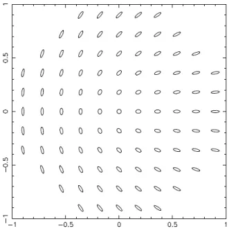
2.2 Sketch of the effect of the convergence and shear on the image of a round source . . . 52

2.3 Tangential and cross components of the shear . . . 53

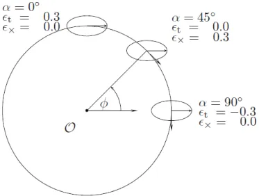
2.4 Shape of the image of a circular source, as a function of the ellipticity components . . . 55

2.5 Reconstruction of the radial surface density contrast . . . 61

2.6 Miscentering parameters from van Uitert et al. (2016) . . . 64

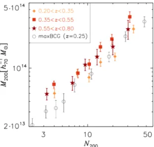
2.7 Mass-richness relation from van Uitert et al. (2016) . . . 65

2.8 Mass-concentration relation from van Uitert et al. (2016) . . . 66

2.9 Shear peak counts . . . 68

2.10 Illustration of simulations for peak counts prediction . . . 68

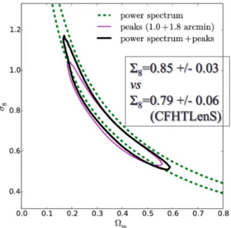
2.11 Constraints on cosmological parameters from peak counts statistics, power spectrum, and joint analysis . . . 69

(9)

2.12 CMB lensing power spectrum measured from different surveys

with increasing significance . . . 72

2.13 Illustrative example of the effects of shear, seeing, pixelization and noise on the image of a galaxy . . . 73

2.14 Scheme of the different ingredients involved in weak lensing analysis . . . 76

2.15 Multiplicative and additive calibration corrections of lensfit ellipticity measurements . . . 77

2.16 Constraints on cosmological parameter obtained with different photometric redshift uncertainty and calibration methods. . . 77

2.17 Comparison of low resolution images from ground based tele-scopes with high resolutions ones from space teletele-scopes . . . . 79

2.18 The tension between Planck CMB and KiDS lensing . . . 81

3.1 Illustration of the bootstrap method . . . 85

3.2 Burn in and converge of MCMC chain . . . 87

3.3 Example of a skewed probability density . . . 89

3.4 Representation of a step of the Stretch Move . . . 90

4.1 Lensing efficiency as a function of cluster redshift, for sources at z = 1 . . . 102

4.2 The richness and redshift distributions of the RedGOLD CFHT-LS W1, NGVS5, and NGVS4 . . . 103

4.3 The distribution of the offsets between the RedGOLD, X-ray and simulation cluster centers . . . 111

4.4 MCMC corner plot . . . 116

4.5 Comparison of the mass-richness relation with that of Ford et al. (2015) . . . 119

4.6 Comparison of the miscentering parameters with those derived by Ford et al. (2015) . . . 120

4.7 The percentage of selected background sources, and the per-centage of wrong selections, as a function of the cluster redshift123 4.8 Mass-richness relations obtained using the different selection criteria . . . 126

4.9 Masses inferred fitting individual clusters with λ > 50 . . . 127

4.10 Number density of background sources as a function of redshift 127 4.11 Mean number density of background sources as a function of redshift and richness. . . 128

4.12 Mass-richness relations obtained fitting different λ bins . . . . 128

4.13 Shear field maps for the stacking of 50, 100, 150 clusters . . . 130

(10)

4.15 Masses of individual clusters obtained with the miscentering

correction, and without . . . 132

4.16 Lensing S/N ratio map of simulations with and without the intrinsic ellipticity . . . 133

4.17 Convergence and S/N ratio map of a simulated cluster . . . . 135

4.18 Optical images and lensing S/N maps of some of the most massive RedGOLD clusters, with centers in good agreement . 137 4.19 Optical images and lensing S/N maps of some of the most massive RedGOLD clusters, with centers not in agreement . . 138

4.20 Comparison of the shear profiles measured with the CFHT-LS W1 + NGVS5, NGVS4, and CFHT-LS W1 + NGVS5 + NGVS4142 4.21 Shear profiles measured with the CFHT-LS W1 + NGVS5 + NGVS4, and the corresponding lensing signal-to-noise ratio maps . . . 144

4.22 Signal contribution to the shear profile . . . 145

4.23 The weak lensing mass-richness relations obtained with the complete sample CFHT-LS W1 + NGVS5 + NGVS4, using the three different models . . . 147

4.24 Effect of the a posteriori intrinsic scatter correction . . . 149

4.25 Comparison of the mass-richness relations derived with and without scatter in the c-M relation . . . 149

4.26 Normalized difference between X-ray masses and lensing masses151 4.27 Comparison between X-ray masses and lensing masses . . . 152

4.28 Mass-luminosity and mass-temperature relations . . . 153

5.1 Comparison of the mass-richness relation derived from the Two Component Model, with the a posteriori intrinsic scatter cor-rection, with others in literature . . . 159

5.2 Comparison of RedGOLD and redMaPPer richnesses as a function of redshift . . . 161

6.1 Stellar mass versus halo mass relation . . . 174

6.2 Optimal filter from Maturi et al. (2005) . . . 176

6.3 Effective convergence power spectrum . . . 177

(11)

LIST OF TABLES

4.1 MCMC priors for the fit of the shear profiles . . . 115

4.2 Mass-richness relation parameters obtained with the different background selection criteria . . . 124

4.3 Difference between the mass-richness relation parameters ob-tained with the different selection criteria . . . 124

4.4 Range in λ, the number of clusters, and the mean λ, for each bin in the different λ binnings . . . 129

4.5 MCMC priors for the joint fit of the shear profiles . . . 139

4.6 Parameters derived for the five models of the joint fit . . . 140

4.7 Stacking background source number density . . . 143

4.8 Parameters derived from the fit of the Basic Model, the Added Scatter Model, and the Two Component Model shear profiles to the measurements . . . 146

4.9 The results of the fit of the mass-richness relation, the nor-malized average difference between lensing and X-ray masses, and the average ratio of the two . . . 148

4.10 Results of the fit of the weak lensing mass versus X-ray mass and mass proxy relations . . . 156

4.11 Comparison of the mass-temperature and mass-luminosity re-lations with others in literature . . . 157

(12)

ABSTRACT

Galaxy clusters are essential cosmological and astrophysical tools, since they represent the largest and most massive gravitationally bound structures in the Universe. Their number and distribution permit us to probe the pre-dictions of cosmological models and structure formation scenarios. Through the study of their mass function, of their correlation function, and of the scaling relations between their mass and different observables, we can infer the cosmological parameters and constrain them. Galaxy clusters are also interesting laboratories that allow us to study galaxy formation and evolu-tion, and their interactions with the intra-cluster medium, being the densest environment that we can find in the Universe.

For all of these goals, an accurate estimate of the cluster mass is of fun-damental importance. Since it cannot be measured directly, we need to rely on mass proxies. Studying galaxy clusters radiation at different wavelengths, we can estimate their mass using different tracers.

The cluster mass can be derived from X-ray observations of the cluster gas, measuring its temperature under the assumption of hydrostatic equilib-rium (Sarazin, 1988). Studying the emission in the millimeter of the intra-cluster medium, we can measure the total intra-cluster mass through the thermal Sunyaev-Zel’dovich effect (S-Z effect; Sunyaev & Zeldovich, 1972). In the optical and in the infrared, we can use the starlight emission of cluster galax-ies. In fact, we can relate the velocity dispersion of cluster members to the cluster mass through the virial theorem, assuming that the cluster is in dy-namical equilibrium. Also the cluster’s total optical or infrared luminosity can be used as a mass proxy. Postman et al. (1996), for example, defined the richness parameter, introduced by Abell (1958), as the number of cluster galaxies brighter than the characteristic luminosity of the Schechter (1976) profile, L∗.

Gravitational lensing is another tool that can be used to measure cluster masses. Strong and weak gravitational lensing produce a distortion of the image of the background sources that it’s proportional to the total cluster mass. In the strong lensing regime, this distortion can be so intense that it creates multiple-image systems or image deformations that can be seen by eye, like Einsteins rings or arcs in galaxy clusters. On the other hand, in the weak lensing regime, the cluster gravitational potential produces small distortions in the observed shape of the background field galaxies, creating the so-called shear field. Because the shear is small relative to the intrinsic ellipticity of the galaxies (due to their random shape and orientation), a statistical approach is required to measure it and the signal is averaged over a large number of background sources to increase the signal-to-noise ratio

(13)

(Schneider, 2005).

Different mass proxies usually lead to mass estimations that are affected by different systematics. X-ray mass measurements are not reliable in sys-tems for which the assumption of the hydrostatic equilibrium is not valid, such as clusters in merging process or in the central regions of clusters with strong AGN feedback. The S-Z method allows us to perform mass measure-ments at high redshifts, but it is subjected to projection effects. Velocity dispersion measurements are not affected by forms of non-thermal pressure such as magnetic fields, turbulence and cosmic ray pressure, as X-ray and S-Z mass measurements, but they are sensitive to triaxiality and projection effects, and constrained to the assumption of dynamical equilibrium. Gravi-tational lensing, on the other hand, does not require any assumption on the dynamical state of the cluster and it is sensitive to the projected mass along the line of sight, representing a more reliable tool to determine total cluster masses (Meneghetti et al., 2010; Allen, Evrard & Mantz, 2011; Rasia et al., 2012).

Every method as its advantages and disadvantages but optical and in-frared detection methods are particularly important since, in the future, large scale surveys at these wavelengths, such as LSST1 _{and Euclid}2 _{will be able}

to identify clusters that will not be detected with other methods.

Several works in the literature have proven that the optical richness shows a good correlation with the cluster total masses derived from weak lensing (Johnston et al., 2007; Covone et al., 2014; Ford et al., 2015; van Uitert et al., 2015; Simet et al., 2016; Melchior et al., 2016). The typical mass uncertainty at a given richness is of ∼ 10 − 25% including statistical and systematic errors, in the mass range 6 × 1012_M

⊙ ≲ M ≲ 1015M⊙ and in the redshift

range 0.1 ≲ z ≲ 0.9.

Rykoff et al. (2014) built an optical cluster finder based on the red-sequence finding technique, redMaPPer, and applied it to the Sloan Digital Sky Survey (SDSS; York et al., 2000). This technique detects galaxy clus-ters looking for overdensities of early type galaxies (ETGs). It relies on the observational evidence that cluster inner regions host a large population of this kind of galaxies, which are tightly distributed on a red-sequence on the color-magnitude diagram (Gladders & Yee, 2000). redMaPPer richness is computed using optimal filtering, as a sum of probabilities and depends on three filters based on colors, positions and luminosity (Rozo et al., 2009a; Rozo & Rykoff, 2014; Rykoff et al., 2012, 2014, 2016).

Licitra et al. (2016a,b) introduced a simplified definition of cluster

rich-1_{http://www.lsst.org}

(14)

ness based on the redMaPPer richness measurement, within their detection and cluster selection algorithm RedGOLD.

This algorithm is based on a revised red-sequence technique. It assigned to each detection the center coordinates, the redshift, a significance parame-ter, and a richness. RedGOLD richness quantifies the number of red, passive ETGs brighter than 0.2L∗, inside a given radius. It is optimized to detect

massive galaxy clusters ( M200 > 1014M⊙), and to produce optical cluster

catalogs with high completes and purity. When compared to X-ray mass proxies, the RedGOLD richness leads to scatters in the X-ray temperature-richness relation similar to those obtained with redMaPPer (Rozo & Rykoff, 2014), which is very promising since RedGOLD was applied to a lower rich-ness threshold (i.e. lower cluster mass).

The goal of my thesis was to measure cluster masses using weak lensing, and derive scaling relations with optical and X-ray mass proxies. This per-mitted me to calibrate and evaluate the precision of the RedGOLD richness as a cluster mass proxy. Using the mean lensing cluster masses calculated stacking clusters in bins of richness, I inferred the mass-richness relation. I then compared the weak lensing masses with X-ray masses, luminosity, and temperature.

For this work, I used the RedGOLD cluster catalogs of the Canada-France-Hawaii Telescope Legacy Survey (CFHT-LS; Gwyn, 2012) Wide 1 (W1) field and of the Next Generation Virgo Cluster Survey (NGVS; Fer-rarese et al., 2012), obtained by Licitra et al. (2016a,b). The algorithm detected 652 clusters on the CFHTLS W1, and 279 and 1704 clusters on the ∼ 20deg2 _{of the NGVS covered by 5 bands and on the entire NGVS without}

the r-band coverage, respectively. For the weak lensing analysis, I selected a subsample of 1323 clusters with a threshold in significance of σdet ≥ 4,

with richness 10 < λ < 70, and redshift 0.2 ≤ z ≤ 0.5. Using this selection, the published catalogs are ∼ 100% complete and ∼ 80% pure Licitra et al. (2016a).

I used the photometric redshift catalogs obtained by Raichoor et al. (2014), with the Bayesian softwares LePhare (Arnouts at al., 1999; Arnouts et al., 2002; Ilbert et al., 2006) and BPZ (Benítez, 2000; Benítez et a., 2004; Coe et al., 2006). They found a bias −0.05 < ∆z < 0.02, scatter values in the range 0.02 < σ < 0.06, and 5 − 15% of outliers, for i′ _{< 23} _mag.

For the shear analysis, I used the CFHTLenS and the NGVSLenS shear catalogs, based on an improved data reduction, compared to the standard THELI pipeline (Erben et al., 2005, 2009, 2013), performed by Raichoor et al. (2014). Galaxy shape measurements were obtained applying the Bayesian lensfit algorithm (Miller et al., 2013).

(15)

(2012), and Piffaretti et al. (2011) X-ray catalogs.

In order to infer weak lensing masses, using the cluster, photometric red-shift, and shear catalogs, I developed and optimized my own weak lensing analysis pipeline. The code starts with the selection of the background galaxy field inside a circular area of a given radius around each cluster in the sam-ple, through a photometric redshift selection. The algorithm stacks clusters according to their richness, and calculates the radial shear profiles, averag-ing the tangential shear in logarithmic radial bins around the center of the stacked samples. It applies lens-source pairs weights (that depend on the lensing efficiency and on the quality of background galaxy shape measure-ments), and the lensfit calibration corrections. The algorithm then calculates the covariance matrices, using the bootstrap method (Efron, 1979), taking clusters with replacements in each richness bin, in order to assign error bars to each point of the radial shear profile. For each stack of clusters, a signal-to-noise ratio map is calculated using aperture mass statistics (Schneider, 1996; Schirmer et al., 2006; Du & Fan, 2014).

Once I obtained the shear profiles for each stack of clusters, I fitted them using Markov Chains Monte Carlo (MCMC; Metropolis et al., 1953). This method allowed me to efficiently sample the model likelihood distribution, from which I obtained the estimation of the error bars on the fitting param-eters and of the confidence regions for each couple of paramparam-eters.

I matched the observed profiles with three analytic models. The Basic Model, which consists of a halo model (Seljak, 2000), with an NFW (Navarro, Frenk & White, 1996) surface density contrast and correction terms that take into account cluster miscentering (Johnston et al., 2007; George et al., 2012), non-weak shear (Mandelbaum et al., 2006; Johnston et al., 2007) and the two halo term (Seljak, 2000; Seljak & Warren, 2004; Johnston et al., 2007). The free parameters of this model are r200, from which I calculate the mass M200,

and the miscentering parameters pcc, and σoff. I then added to this model

an additional free parameter, σM |λ, the intrinsic scatter in the mass-richness

relation (hereafter Added Scatter Model). Finally, I took into account the contribution from the Brightest Central Galaxy (BCG) mass MBCG, adding

this parameter to the Basic Model (hereafter Two Component Model). For the three models, I obtained the mass-richness relation fitting the lensing mass values recovered for each richness bin.

I validated my code comparing my results with those of Ford et al. (2015), obtained in an independent way, using the entire CFTHLS W1, W2, W3, W4, and the public cluster catalog of Milkeraitis et al. (2010), and performed several tests to estimate possible biases in the results. I tested different kinds of background sample selection and source magnitude cuts. I tested the redshift selection and different binnings in richness of the cluster sample. I

(16)

checked that the behavior of the tangential and cross components of the shear profiles were as expected from theory. I compared masses estimated with and without the miscentering correction, in order to evaluate the contribution of this correction term. I used aperture mass statistics to test the identification of cluster centers through the lensing signal, using simulated shear maps, simulated clusters, and observed RedGOLD clusters. In order to check that fitting the profile of each richness bin individually does not introduce a bias in the determination of the mass-richness relation parameters, I tested a joint fit (i.e. the fit of the profiles associated to all richness bin simultaneously).

From the tests that I performed, I concluded that : (1) the joint and individual fitting techniques are equivalent. (2) The miscentering correction is the one that most affects the halo mass measurements. (3) The BCG mass and the intrinsic scatter in the mass-richness relation are not constrained by the data. (4) The BCG mass addition in the model doesn’t affect the recovered halo mass.

For these reasons, I decided to use the mass-richness relation inferred from the Two Component Model, with an a posteriori intrinsic scatter correction (Ford et al., 2015) Final Model. With this model, I obtained a mass-richness relation of log M200/M⊙ = (14.46±0.02)+(1.04±0.09) log (λ/40) (statistical

uncertainties). This result is consistent within 1 − 2σ with the lensing mass-richness relations obtained by Rykoff et al. (2012), Saro et al. (2015), Simet et al. (2016), Farahi et al. (2016) and Melchior et al. (2016), using the SDSS and DES redMaPPer cluster samples.

For the lensing mass vs X-ray luminosity relation I found log  M200E(z) 8×1013_h−1_M_⊙  = (0.10_{± 0.03) + (0.61 ± 0.12) log}  LX 5.6×1042_h−2_erg/sE(z)  . For the lensing mass vs X-ray temperature relation I obtained log  M200E(z) 6×1013_h−1_M_⊙  = (0.23 _{± 0.03) + (1.46 ± 0.28) log} TX 1.5KeV  . These results are consistent with those of Leauthaud et al. (2010), Kettula et al. (2015), Mantz et al. (2016). For all three relations, I found a scatter of 0.20 dex, consistent with redMaPPer scatters.

In the remaining months of my PhD, I will focus on projects that are complementary to what I’ve done so far. I will study the relation between the lensing halo mass and the BCG stellar mass. I will check how different kinds of BCG selection affect the estimated lensing masses, and calculate the stellar-to-halo mass ratio for cluster central galaxies. I will also be able to infer an optical mass-luminosity relation, with the information on the b rest frame luminosity of central galaxies and of the entire cluster.

On the other hand, I would like to study in more detail the miscentering problem to see how different center choices would affect the shear profiles and the mass measurements of stacked or individual massive clusters. I

(17)

would like to expand the work of George et al. (2012) and include in the comparison also centers based on the peak of the weak lensing signal and on the hybrid approach between galaxy centers and centroids (used for example in RedGOLD), not considered in the cited work.

For these new projects I will use the new self calibrating version of the lensfit algorithm, and refined photometric redshift estimations on the CFHTLS W1 and on entire NGVS.

Next generation space surveys as Euclid and WFIRST3 _{will have a huge}

impact on the kind of weak lensing analysis that I performed for my thesis work, giving access to a cluster sample of one order of magnitude bigger. Also, the next generation radio surveys such as SKA4 _{will allow us to extend}

weak lensing measurements to the radio band, and to even larger scales. The aim for future analysis is to reach an accuracy of 1% in cluster mass measurements. The main challenge in weak lensing analysis comes from the photometric redshift estimation that is linked to the selection of background source samples and to the weights assigned to each lens-source pair. In my future work I would like to study how the use of the photometric redshift dis-tribution derived with different calibration methods affect the measurement of weak lensing masses and of cluster lensing centers.

The thesis is organized as follows: in Chapter 1, I will discuss galaxy clusters from a theoretical and observational point of view. I will describe the standard cosmological model, the structure formation mechanism, the most used cluster mass profiles, and the cluster mass function. I will also talk about how we can detect galaxy clusters and estimate their mass using different mass proxies, and the importance of scaling relations. In Chapter 2, I will summarize the theoretical principles of weak lensing, and discuss its possible applications. In Chapter 3, I will explain the statistical methods that I used for my analysis and the way that I applied them to the data. In Chapter 4, I will describe in detail the analysis and the tests that I performed. Finally, in Chapter 6, I will summarize the main results of my thesis work, discuss my future projects, and the perspectives of the weak lensing field.

3_{http://wfirst.gsfc.nasa.gov}

(18)

RÉSUMÉ

Les amas de galaxies sont des outils cosmologiques et astrophysique essen-tiels, car ce sont les objets les plus grands et les plus massifs gravitationnelle-ment liées dans l’Univers. Leur nombre et leur distribution nous permettent de tester les prévisions des modèles cosmologique et les scenarii de formation des structures. Par l’étude de leur fonction de masse, de leur fonction de cor-rélation et des relations d’échelle entre leur masse et différentes observables, nous pouvons contraindre les paramètres cosmologiques de façon toujours plus stricte. En tant qu’environnements les plus denses qu’y soit dans l’Uni-vers, les amas de galaxies sont aussi d’intéressants laboratoires pour l’étude de la formation et de l’évolution des galaxies, et de leur interactions avec le milieu qui les entourent.

Pour y parvenir, estimer précisément leur masse revêt une importance fondamentale. Puisqu’elle ne peut pas être mesurée directement, nous devons compter sur d’autres observables appelés alors mass proxy.

Avec les différentes longueurs d’onde auxquelles l’amas est observée viennent différents mass proxy. La masse d’un amas peut être dérivée de l’observation du gaz de l’amas en rayon X, en mesurant sa température avec l’hypothèse que ce dernier est en équilibre hydrostatique (Sarazin, 1988). En étudiant l’émission millimétrique du milieu intra-amas, nous pouvons mesu-rer la masse totale à l’aide de l’effet Sunyaev-Zel’dovich thermique (effet S-Z ; Sunyaev & Zeldovich, 1972). En optique et en infra-rouge, c’est l’émission des étoiles de l’amas qui nous renseigne : la mesure de la dispersion de vitesse des membres de l’amas et la masse totale peut être mis en relation, lorsque celui ci s’applique, avec le théorème du viriel. La luminosité en optique et en infra-rouge peuvent aussi être utilisés comme de mass proxy. On définit alors, à la manière de Abell (1958) et Postman et al. (1996) par example, le paramètre de richesse comme le nombre de galaxies d’amas plus brillantes que la luminosité caractéristique du profil de Schechter (1976), L∗.

L’effet de lentille gravitationnelle est un autre outil qu’on peut utiliser pour mesurer la masse des amas. L’effet de lentille gravitationnelle fort et l’effet de lentille gravitationnelle faible (i.e. strong lensing et weak lensing, respectivement), produisent une distorsion de l’image des sources en arrière plan proportionnelle à la masse totale de l’objet d’avant plan, ici un amas de galaxies. Dans le régime de strong lensing d’une part, cette distorsion peut être si intense qu’elle crée un système d’images répliquées ou une dé-formation de l’image qui peuvent être aisément identifiées à l’œil, comme les anneaux d’Einstein ou les arcs dans les amas de galaxies. Dans le régime du weak lensing d’autre part, le potentiel gravitationnel produit de plus faibles distorsions qui affectent la forme observée de la galaxie d’arrière plan. Ces

(19)

déformations sont quantifiées par le biais de ce que l’on nomme champ de shear. Comme ce dernier est faible devant la grande diversité de morphologie et d’orientation des galaxies, il faut adopter une approche statistique pour le mesurer et ainsi calculer la moyenne sur un grand nombre de sources d’arrière plan (Schneider, 2005).

Différents mass proxy mènent généralement à des estimations de masse qui sont affectées par des différences systématiques. Les mesures de masse en rayon X faillissent dans les systèmes où l’hypothèse d’équilibre hydrosta-tique n’est pas applicable, comme les amas en cours de fusion ou dans les régions centrales lorsque l’effet d’un noyaux actif de galaxie (AGN ) est im-portant. La méthode S-Z quant à elle, nous permet de faire des mesures de masse à haut décalage spectral (redshift), mais elle est affectée par des effets de projection. Contrairement aux deux méthodes précédentes, les mesures de dispersion de vitesse ne sont pas impactées par les formes de pression non-thermique comme les champs magnétiques, la turbulence et la pression des rayons cosmiques, mais elle sont sensibles à l’asymétrie du potentiel et aux effets de projection en plus de reposer sur l’hypothèse que le système est à l’équilibre dynamique. L’effet de lentille gravitationnelle, par contre, ne souffre d’aucun de ces écueils. Il est directement sensible à la masse totale projetée sur la ligne de visée, et représente donc un outil fiable pour la déter-mination de la masse totale des amas (Meneghetti et al., 2010; Allen, Evrard & Mantz, 2011; Rasia et al., 2012).

Chacune de ces méthodes offre des avantages et présente des inconvénients mais les méthodes de détection en optique et en infra-rouge sont particulière-ment importantes car, dans le future, les programmes d’observations à grande échelle dans ces longueurs d’onde, comme LSST et Euclid, seront capables d’identifier des amas qui ne sauraient être détectés autrement.

Plusieurs travaux ont démontré que la richesse optique présente une bonne corrélation avec la masse totale de l’amas mesurée avec le weak len-sing (Johnston et al., 2007; Covone et al., 2014; Ford et al., 2015; van Uitert et al., 2015; Simet et al., 2016; Melchior et al., 2016). L’incerti-tude caractéristique sur la masse, à richesse fixée, est de ∼ 10 − 25%, cela inclue les erreurs statistiques et systématiques, dans l’intervalle de masse 6_{× 10}12M⊙ ≲ M ≲ 1015M⊙ et dans l’intervalle de redshift 0.1≲ z ≲ 0.9.

Rykoff et al. (2014) ont développé redMaPPer, un algorithme optique de détection d’amas basé sur la technique de la sequence rouge, algorithme qu’ils ont appliqué aux Sloan Digital Sky Survey (SDSS ; York et al., 2000). Cette méthode identifie les amas de galaxies en détectant les surdensités de galaxies early type (ETGs). Les observations montrent en effet que la région centrale d’un amas accueille un grande nombre de galaxies de ce type, ces dernières sont, lorsqu’on les placent dans un diagramme couleur - magnitude,

(20)

distribuées dans une étroite région appelée la séquence rouge. La richesse de redMaPPer est définie comme une somme de probabilité et utilise un filtrage en couleur, position et luminosité (Rozo et al., 2009a; Rozo & Rykoff, 2014; Rykoff et al., 2012, 2014, 2016).

Licitra et al. (2016a,b) ont par la suite présenté une définition simplifiée de la richesse basée sur celle de redMaPPer et l’ont utilisé pour bâtir RedGOLD, leur algorithme de détection d’amas.

Cet algorithme est fondé sur une technique de sequence rouge révisée ; il estime à chaque détection d’un amas les coordonnées de son centre, son redshift, un paramètre dit de confiance et sa richesse. La richesse de Red-GOLD quantifie le nombre de ETGs rouge et passives, plus brillantes que 0.2L∗, dans un rayon donné. Il est optimisé pour détecter des amas de

ga-laxies massifs (M200 > 1014M⊙), et pour produire des catalogues optiques

complets et purs. Comparés aux résultats obtenues via des observations en rayon X, la richesse définie dans RedGOLD conduit à des dispersions dans la relation temperature X - richesse qui sont similaires à celles obtenues avec redMaPPer (Rozo & Rykoff, 2014), ce qui est très prometteur étant donné que RedGOLD a été appliqué avec un seuil en richesse inférieur (soit sur des amas de masse inférieure).

L’objectif de mon travail de thèse était de mesurer des masses d’amas en utilisant le weak lensing ainsi d’établir les relations entre la masse totale d’une part et la richesse, la luminosité X, la température X et la masse X d’autre part. On parle alors de relation d’échelle. Cela m’a permis de calibrer et valider la précision de la richesse de RedGOLD en tant que mass proxy. J’ai inféré la relation masse - richesse, en utilisant les masses weak lensing moyennes calculées en empilant les amas en groupes de richesse. Ensuite j’ai comparé mes masse weak lensing avec de masse, luminosités et temperatures en rayon X.

Pour ce travail, j’ai utilisé les catalogues d’amas de RedGOLD des cam-pagnes d’observations du Canada-France-Hawaii Telescope Legacy Survey (CFHT-LS ; Gwyn, 2012) Wide 1 (W1) et Next Generation Virgo Cluster (NGVS ; Ferrarese et al., 2012), obtenus par Licitra et al. (2016a,b). L’al-gorithme a détecté 652 amas dans le CFHTLS W1 et, pour le NGVS, 279 amas dans la portion de ∼ 20 degrés carrés observée dans 5 bandes et 1704 dans l’intégralité du champ observé sans la bande r. Pour l’analyse weak len-sing, j’ai sélectionné un échantillon de 1323 amas, au dessus d’un seuil de détection σdet ≥ 4, dans l’intervalle de richesse 10 < λ < 70 et de redshift

0.2 _{≤ z ≤ 0.5. En utilisant cette sélection, les catalogues publiés sont ∼ 100%} complets et ∼ 80% purs (Licitra et al., 2016a).

J’ai utilisé les catalogues de redshift photométriques obtenus par Rai-choor et al. (2014), avec les logiciels bayésiens LePhare (Arnouts at al.,

(21)

1999; Arnouts et al., 2002; Ilbert et al., 2006) et BPZ (Benítez, 2000; Benítez et a., 2004; Coe et al., 2006). Ces derniers ont déterminé un biais −0.05 < ∆z < 0.02, une valeur de dispersion 0.02 < σ < 0.06, et 5 − 15% de points aberrants, pour i′ _{< 23} _magnitude.

Pour mon analyse, j’ai utilisé les catalogues de shear CFHTLenS et NGVSLenS, basés sur une analyse de données plus sophistiquée comparée à la procédure THELI standard (Erben et al., 2005, 2009, 2013), réalisée par Raichoor et al. (2014). Les mesures de formes des galaxies ont été ensuite obtenues en appliquant l’algorithme bayésien lensfit (Miller et al., 2013).

Pour effectuer la comparaison avec les observations en rayon X, j’ai utilisé les catalogues de Gozaliasl et al. (2014) et Mehrtens et al. (2012).

Pour obtenir les masses weak lensing à partir de catalogues d’amas, de redshift photométriques et de shear, j’ai développé et optimisé ma propre procédure d’analyse. Tout d’abord, l’algorithme fait la sélection des galaxies d’arrière plan dans une région circulaire de rayon donné autour du centre de chaque amas de l’échantillon à l’aide des redshift photométriques. L’al-gorithme empile ensuite les amas selon leur richesse et il calcule les profils de shear radiaux, en faisant la moyenne des shear tangentielles dans des in-tervalles logarithmiquement espacés autour du centre de l’échantillon empilé. Cette moyenne inclue des coefficients qui dépendent de l’efficacité de l’effet de lentille produit par l’amas, de la qualité des mesures des déformations subit par l’image de la source d’arrière plan ainsi que de corrections de calibration opérées par lensfit. Ensuite mon logiciel calcule les matrices de covariance, par la méthode dite de bootstrap (Efron, 1979), qui consiste à réaliser un tirage avec remise d’amas dans chaque intervalle de richesse afin d’assigner une barre d’erreur à chaque point du profile radial de shear. Pour chaque regroupement d’amas, une carte du rapport signal sur bruit est produite en utilisant la statistique dite d’aperture mass (Schneider, 1996; Schirmer et al., 2006; Du & Fan, 2014).

Une fois les profils de shear obtenus pour chaque pile d’amas, j’ajuste un modèle sur chacun grâce à un algorithme de chaînes de Markov Monte Carlo (MCMC ; Metropolis et al., 1953). Cette méthode me permet d’échantillonner efficacement la distribution de vraisemblance du modèle, de laquelle je tire une estimations et une barre d’erreur pour chaque paramètre ainsi que des intervalles de confiance pour chaque couple de paramètres.

Dans une premier temps, j’ajuste aux profils observés un modèle basique (ci-après Basic Model) qui consiste en un modèle de halo (Seljak, 2000), avec un contraste de densité superficiel NFW (Navarro, Frenk & White, 1996) et un termes de correction qui tient compte de l’erreur sur le centrage de l’amas (miscentering ; Johnston et al., 2007; George et al., 2012), les non-weak shear (Mandelbaum et al., 2006; Johnston et al., 2007) et le two-halo term (Seljak,

(22)

2000; Seljak & Warren, 2004; Johnston et al., 2007). Les paramètres libres de cette modèle sont r200 (duquel je déduit la masse M200), le paramètres dit

de miscentering, pcc et σoff.

À ce premier modèle, j’ai ensuite ajouté un paramètre supplémentaire,

σ_{ln M |λ}, qui caractérise la dispersion intrinsèque dans la relation

masse-richesse. Cela donne le Added Scatter Model.

Indépendamment, j’ai pris en compte la contribution de la galaxie la plus brillante (nommé BCG) à la masse totale, et ajouté pour ce faire le paramètre libre MBCG au Basic Model pour obtenir le Two Component Model.

La masse prédite pour chaque regroupement d’amas par chacun des trois modèles me permet ensuite d’établir une relation entre masse et richesse.

J’ai ensuite validé mon code en comparant mes résultats avec ceux de Ford et al. (2015), obtenus de façon indépendante, en utilisant le CFHTLS W1, W2, W3, W4 entier, et le catalogue d’amas publique de Milkeraitis et al. (2010). J’ai effectué plusieurs tests afin d’écarter d’éventuels biais dans mes résultats. J’ai notamment testé différents critères de sélection pour l’échan-tillon de sources d’arrière plan et différentes limites en magnitude. J’ai vérifié la sélection en redshift et la façon d’échantillonner les amas en fonction de leur richesse. J’ai contrôlé que le comportement des composantes ortho-radiales du shear étaient conforme aux prédictions théoriques. J’ai comparé les masses estimées avec et sans la correction de miscentering afin d’évaluer sa contri-bution. J’ai utilisé la statistique d’aperture mass pour tester l’identification des centres des amas à l’aide du signal de lensing, en utilisant des cartes de shear simulées, d’amas simulés et d’amas observés par RedGOLD. Afin de vérifier qu’en ajustant le profil de chaque intervalle de richesse individuelle-ment nous n’introduisons pas un biais dans la détermination des paramètres de la relation masse - richesse, j’ai essayé d’ajuster l’ensemble des intervalles de richesses simultanément.

Mes test m’ont permis de conclure que : (1) les techniques d’ajustement individuel et simultané sont équivalentes. (2) La correction de miscentering est celle dont l’impact sur la mesure de la masse est le plus grand. (3) La masse de la galaxie centrale (BCG) et la dispersion intrinsèque dans la re-lation masse - richesse ne sont pas contraintes par les données. (4) L’ajout de la masse de la BCG dans le modèle n’affecte pas l’estimation de la masse totale de l’amas.

Pour cette raisons, j’ai décidé d’utiliser la relation masse - richesse infé-rée par le Two Component Model, avec un correction a posteriori pour la dispersion intrinsèque (Ford et al., 2015) (Final Model). Avec ce modèle, j’ai obtenu la relation masse-richesse log M200/M⊙ = (14.46± 0.02) + (1.04 ±

0.09) log (λ/40) (erreurs systématiques). Ce résultat est cohérent à 1 − 2σ avec les relations masse - richesse lensing obtenues par Rykoff et al. (2012),

(23)

Saro et al. (2015), Simet et al. (2016), Farahi et al. (2016) et Melchior et al. (2016), en utilisant les échantillons d’amas obtenus par redMaPPer avec le SDSS et le DES.

Pour la relation Mlens

200 − M200X , pour une pente unitaire fixé, j’ai obtenu

log M₂₀₀lens = (0.20_{± 0.03) log M}₂₀₀X . Pour la relation masses lensing - lumino-sité en rayons X j’ai trouvé log M200E(z)

8×1013_h−1_M_⊙  = (0.10 _{± 0.03) + (0.61 ±} 0.12) log  LX 5.6×1042_h−2_erg/sE(z) 

. Pour la relation masses lensing - tempéra-ture en rayons X j’ai obtenu log M200E(z)

6×1013_h−1_M_⊙  = (0.23_{± 0.03) + (1.46 ±} 0.28) log TX 1.5KeV 

. Ces résultats sont en accord avec ceux de Leauthaud et al. (2010), Kettula et al. (2015), Mantz et al. (2016). Pour ces trois relations, j’ai trouvé une dispersion de 0.20 dex, ce qui est compatible avec les dispersions de redMaPPer.

Au cours des derniers mois de mon doctorat, je me concentrerai sur des projets complémentaires à ce que j’ai fait jusqu’ici. J’étudierai la relation entre les masses lensing des halos et les masses stellaires des BCG. Je véri-fierai comment différents critères de sélection de la galaxie BCG affectent les masses estimées avec le lensing, et je calculerai le rapport masse du halo sur masse stellaire pour les galaxies centrales des amas. Je serai aussi en mesure de déduire la relation masse - luminosité optique avec la luminosité en bande b soit pour l’objet central soit pour l’ensemble de l’amas.

D’un autre côté, j’aimerai étudier plus en détail le problème du miscente-ring pour voir comment différents choix de centrage affectent les profiles de shear et les mesures de masse d’amas massifs, individuels ou empilés. J’ai-merai étendre le travail de George et al. (2012) et y inclure une comparaison avec une technique de centrage utilisant le weak lensing et une reposant sur une approche hybride entre l’utilisation de galaxies et de centroïdes comme centres (utilisé par example dans RedGOLD), méthodes non considérées dans le travail cité.

Pour ces nouveaux projets, j’utiliserai la nouvelle version auto calibrante de l’algorithme lensfit, et des estimations raffinées de redshifts photomé-triques de CFTHLS W1 et de l’intégralité de NVGS.

Les programmes d’observations spatiaux de nouvelle génération comme Euclid et WFIRST auront un énorme impact sur les analyses de données de weak lensing telles que les ai conduites au cours de mon travail de thèse. Ils donneront accès à un échantillon d’amas un ordre de grandeur plus im-portant. Sans compté les campagnes en radio de nouvelle génération tel que SKA qui permettront d’étendre les mesures de masses weak lensing en bande radio à des échelles spatiales plus grande encore.

(24)

pourcent sur les mesures de masses des amas. Le principal défi dans le trai-tement des données issues du weak lensing vient de l’estimation du redshift photométriques qui est liée à la sélection de l’échantillon de sources d’arrière plan et aux coefficients assignés à chaque paire lentille-source. Dans mon travail futur j’aimerai étudier comment l’utilisation de la distribution de red-shift photométriques obtenue par différentes méthodes de calibration affecte les mesures de masse weak lensing et la position estimée du centre des amas. Cette thèse est organisée comme suit : dans le Chapitre 1, je présenterai les amas de galaxies d’un point de vue théorique et observationnel. Je décrirai le modèle cosmologique standard, le mécanisme de formation des structures, les profils de masse les plus couramment utilisés, et la fonction de masse des amas. Je discuterai aussi des techniques employées pour détecter les amas de galaxies et estimer leur masse en utilisant différents estimateurs (mass proxy), ainsi que l’importance des relations d’échelle. Dans le Chapitre 2, je résumerai les principes théoriques du weak lensing, et je présenterai ces applications possibles. Dans le Chapitre 3, j’expliquerai les méthodes statistiques que j’ai mises à profit pour mon analyse et la manière dont je les ai appliquées aux données. Dans le Chapitre 4, je discuterai en détail l’analyse et les tests que j’ai réalisés. Enfin dans le Chapitre 6, je résumerai les principaux résultats de mon travail de thèse, je discuterai mes projets futurs et les perspectives du domaine d’étude des lentilles gravitationnelles faibles.

(25)

CHAPTER

ONE

GALAXY CLUSTERS

Galaxy clusters are the the largest and the most massive gravitationally bound systems in the Universe. They have proven to be important tools to probe the predictions of cosmological models and structure formation sce-narios. They also permit us to study galaxy formation and evolution, and their interactions with the intra-cluster medium, in a dense environment. Their number and distribution allows us to study the mass function and the correlation function, from which we can infer the cosmological parameters. Studying with accuracy the scaling relations between cluster mass, and dif-ferent observables, we can put even tighter constrains on the cosmological model.

In this chapter, I will start by describing the standard cosmological model and the evolution of its components. I will explain the process of cluster formation through the growth of the density perturbations in non linear regime. I will discuss clusters from a theoretical point of view, their profile and mass function, and from an observational point of view, reviewing the main methods to detect them and infer their masses through mass proxies.

1.1 Theory

1.1.1 Cosmological model

Cosmology is the study of the Universe and of the formation, evolution, and interaction of its components, from galaxies and clusters to the large scale structure.

Modern cosmology is based on the cosmological principle that states that the Universe is homogeneous and isotropic at scales larger than ∼ 100Mpc.

(26)

This means that at large scales the Universe appears the same in all direc-tions, and therefore doesn’t have a center and neither a privileged observing position.

In the context of General Relativity, such a universe can be described by the Friedmann-Robertson-Walker metric:

ds2 = c2dt2_{− a(t)}2dr2+ Sk(r)2dΩ2

 with dΩ2 _{≡ dθ}2_{+ sin}2_θϕ2 _{and S}

k a function of the curvature of space-time:

Sk(r) =        R sin (r/R) f or k = +1 r f or k = 0 R sinh (r/R) f or k =₋₁

where k is the curvature constant (that corresponds, for the three cases listed, to a positively curved, flat and negatively curved space, respectively) and R is the curvature radius.

a(t) is the scale factor that describes how distances expand or contract as a function of time, in an homogeneous and isotropic universe.

In 1929, in fact, Hubble discovered that the Universe is expanding. Con-sidering that the light emitted by galaxies is shifted toward longer wave-lengths when observed by us, the redshift of a galaxy can be defined as:

z _≡ λob− λem λem

Hubble derived a linear relation between redshift and distance, known today as the Hubble’s law:

z = H c r

where H = ˙a/a is the Hubble constant and a(t) is the scale factor introduced above that, at present time is equal to one. In an homogeneous and isotropic universe in expansion, the scale factor ensures that relative distances are preserved.

We can also define the Hubble distance as DH = c/H that is a good

approximation of the horizon, the maximum distance that a photon can travel during the age of the universe.

In 1922, Friedmann derived an equation to describe such a universe in expansion using Einstein’s field equation:

 ˙a a 2 = 8πG 3 ρ− kc2 a2 + Λc2 3

(27)

¨ a a =− 4πG 3  ρ +3p c2  +Λc 2 3

where ρ and p are the density and the pressure of the fluid, G is the gravita-tional constant, c is the speed of light, and Λ is the cosmological constant.

Considering a flat universe composed by radiation, matter, and a cosmo-logical constant, we can rewrite Friedmann’s equation as:

 ˙a a 2 = 8πG 3 (ρm+ ρr+ ρΛ)

with ρm = ρDM + ρb, meaning that the matter component is composed by

dark matter and baryons. The densities ρm, ρr, ρΛ, ρDM, ρb are the densities

of matter, radiation, dark energy, dark matter, and baryons, respectively. Furthermore, defining the Hubble constant at present time as H0 =

( ˙a/a)t=t0, and the critical density of the universe as ρc,0 = 3H

2

0/8πG, the

equation takes the form: H2 H2 0 = Ωm a3 + Ωr a4 + ΩΛ

where the density parameter for each component x is Ωx = ρx,0/ρc,0, and

their sum is Ω = Ωm + Ωr + ΩΛ = 1. The evolution of the density as a

function of the scale factor is given by the continuity equation: ρ(a) = ρ0 a3(1+w) and w =        0 matter 1/3 radiation −1 Λ

The standard cosmological model assumed today is the Λ − CDM. It’s a spatially flat model that contains baryonic and dark matter, radiation and a dark energy (whose impact on the Universe dynamic is quantified by the cosmological constant), with the Hubble constant assumed to be H0 =

70 km s−1 M pc−1.

The total matter density parameter is Ωm ∼ 0.3 and includes

contribu-tions from both dark matter and baryons, where the density parameter of the first is ∼ 6 times greater than the second.

The radiation density parameter is Ωr ∼ 10−5 and includes neutrinos and

(28)

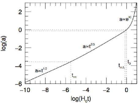
Figure 1.1 – In the table on the top, the density parameter of the different components of the Λ_{− CDM model. In the table on the bottom, the scale} factor, time, redshift, and temperature at which the main events took place (Ryden, 2006).

(29)

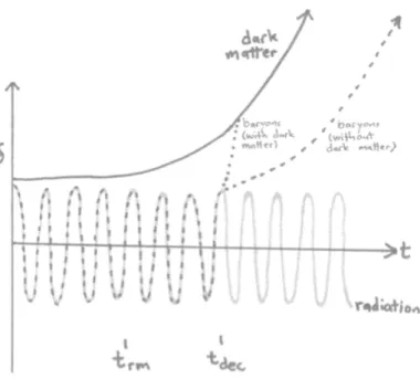
Figure 1.2 – Dependance of the scale factor with time for the different epochs. trm is the radiation-matter equality, tmΛ is the matter-Λ equality, and t0 is

the present time (Ryden, 2006).

Finally the cosmological constant density parameter is ΩΛ∼ 0.7.

In Figure 1.1, we find the density parameter values of the different com-ponents and the scale factor, time, redshift, and temperature at which the main events took place. In Figure 1.2, we can see how the scale factor, and thus the expansion of the Universe, depends on time in the different epochs: radiation, matter, Λ and present time.

Given a cosmological model, there are several ways to measure cosmolog-ical distances.

Following Hogg (2000), we define the comoving line-of-sight distance to an object at redshift z as:

DC = DH  z 0 dz′ E(z′₎ (1.1) where E(z) ≡ H(z)/H0(z) =  Ωm(1 + z)3+ Ωk(1 + z)2+ ΩΛ, DH is the

Hubble distance previously defined, and Ωk = 1−Ωm−Ωr−ΩΛis the density

parameter associated to the curvature constant. The transverse comoving distance is defined as:

(30)

DM =        DH√1_Ω k sinh ( √ ΩkDC/DH) f or Ωk> 0 DC f or Ωk= 0 D_H√1 Ωk sin ( √ Ω_kD_C/D_H) f or Ω_k< 0 (1.2) so that the comoving distance between two objects at the same redshift, separate on the sky by an angle δθ will be DMδθ.

The angular diameter distance of a given object is defined as the ratio of its physical transverse size, l, to its angular size in radians, θ, and it is related to the transverse comoving distance:

DA ≡ l/θ =

DM

(1 + z) (1.3)

Finally, the luminosity distance is defined as the relation between the bolometric (i.e. integrated over all frequency) luminosity L, and the bolo-metric flux S, of an object. It is related to the transverse comoving distance and to the angular diameter distance:

DL≡  L 4πS = (1 + z)DM = (1 + z) 2_D A (1.4)

1.1.2 Density perturbations and structure formation

In the standard model, the primordial Universe was very dense and hot (T >> 104_K_{) so that the baryonic matter was completely ionized, and the}

photons scattering by free electrons made it completely opaque. In the very first phases of its evolution its density was dominated by the radiation den-sity, then, as it expanded the matter density dominated and finally the dark energy density, which is the dominant component today.

While expanding, the average Universe temperature cooled to ∼ 3000K and, at this point, ions and electrons combined to form neutral atoms (re-combination epoch), photons started to stream freely from the so called last scattering surface, decoupling from the electrons, and the Universe became transparent. We observe the photons from the last scattering surface as a Cosmic Microwave Background (CMB; Penzias & Wilson, 1965) with a black body distribution at a temperature of ∼ 2.7K. The CMB shows tempera-ture fluctuations that correspond to matter density perturbations (Planck Collaboration IX, 2016).

Cosmic structures form from gravitational instability and the subsequent growth of these primordial density perturbations. The study of the large

(31)

scale structure in the Universe and its formation is linked to the study of the statistical properties of the overdensity field:

δ(⃗x) = ρ(⃗x)− ρb ρb

where ρb is the average density of the universe.

Assuming that δ(⃗x) is an homogeneous and isotropic Gaussian random field, we can think of our Universe as a statistical realisation of the over-density field, and of its unperturbed over-density as the mean over the statistical ensemble, ρb ≡ ⟨ρ(⃗x)⟩. Moreover, the Gaussian assumption implies that to

completely describe the field, we only need its variance.

In practice, with the ergodic hypothesis, we can calculate ρb averaging the

overdensity field in finite volumes of the Universe that are sufficiently distant to be considered independent (Coles & Lucchin, 2002).

Averaging in a finite volume V is equivalent to filter the overdensity field on a given scale R (Voit, 2005):

δM(⃗x)≡

δM (⃗x)

M = δ(⃗x)∗ W (⃗x; R)

where W (⃗x; R) is a generic window function, and δM is the mass fluctuation.

Considering that luminous matter traces the total matter distribution, we can link the number of galaxies in a given volume V with the corresponding total mass fluctuation in the same volume through the bias parameter b, so that δg ≡ bδM.

We can then write the mass variance as: σ2 _≡δ2(⃗x) = 1

(2π)3



P (k)_{|W (kR)|}2d3k

where P(k) is the power spectrum, the Fourier transform of the correlation function ξ(r) ≡ ⟨δ(⃗x)δ(⃗x + ⃗r)⟩.

Assuming that the power spectrum has a power-law form, P (k) ∼ kn _and

that the window function is a spherical one, we have: σ2 _{∼ k}n+3_→ δM

M ∼ M

−(n+3)/6

The growth of the perturbations doesn’t depend on the scale and they all grow in unison until they are outside of the horizon, where the only important effect is gravity. In this regime, the different components of the Universe are coupled to the dominant one, so in the radiation dominated epoch δ ∝ δr ∝ a2

(32)

Figure 1.3 – Growth of the perturbations inside the horizon, as a function of time (Ryden, 2006).

As time passes and perturbations of larger scales enter in the horizon, new physical effects that modify the scale-free nature of the initial power spectrum need to be taken into account. As we can see in Figure 1.3, before the radiation-matter equality (trm) and inside the horizon, the dominant

component is the radiation, and the baryonic component is coupled to it. Radiation pressure resists gravitational compression, inhibiting the growth of the perturbations. The photo-baryonic fluid oscillates as acoustic waves, and eventually damps because of photon diffusion, while the dark matter component stalls at the amplitude at which it entered the horizon.

After the radiation-matter equality, when the Universe becomes matter dominated, dark matter perturbations start to grow again. The baryons, after decoupling from the photons (tdec), are attracted by the gravitational

wells of dark matter, and catch up with the perturbation growth of this component, while radiation continues to oscillate.

All the alterations that these effects produce on the original power spec-trum, until we are in linear regime, can be described by the transfer function (Voit, 2005):

T (k)_≡ δk(z = 0) δ_kD(z)

(33)

where D(z) is the growth function: D(a)_∝ δρ ρ ∝ ˙a a  a 0 da ˙a3 a = 1 (1 + z)

If the primordial power spectrum has a power law index of n=1, the power spectrum of linear perturbations is P (k) ∝ kn_T2_(k)_{, at z=0 (Voit, 2005).}

In the Λ−CMD model, structure formation is driven by the growth of the dark matter density perturbations and it leads to a hierarchical or bottom-up scenario, in which small scale perturbations reach the nonlinear regime before larger-scale ones (Ryden, 2006). This can be explained by the fact that, before the radiation-matter equality, dark matter perturbations with wavelengths greater than the Hubble distance (small scales in the Fourier space) will be free to grow, while perturbations with smaller wavelengths that are then inside the horizon (large scales in the Fourier space), will stall until the matter dominated epoch.

Figure 1.4 – Power spectrum at the radiation-matter equality for a cold dark matter model (CDM), and for a hot dark matter model (HDM), compared with the scale free power spectrum, P _{∝ k (Ryden, 2006).}

In Figure 1.4, we can see that the power spectrum at the time of radiation-matter equality is suppressed in amplitude for large wavenumbers. This means that galaxies form first, then clusters, and then the large scale struc-ture. This scenario is consistent with the observed ages of galaxies and clusters.

(34)

1.1.3 Cluster formation

As small clumps of matter merge and coalesce to form larger structures, perturbations reach the nonlinear regime with δ ∼ 1. At this point is no longer possible to study the evolution of the perturbations in linear regime and we need to rely on numerical simulations. In a simplified way though, cluster formation can also be studied assuming a spherically symmetric model as the spherical top-hat.

In this model, the radius of a mass shell with constant density has a parametric solution:

r = rta

(1_{− cos θ)} 2

where rta is the turnaround radius at which the expansion stops, and the

collapse starts. The behavior of the radius of a nonlinear perturbation is shown in Figure 1.5.

Figure 1.5 – Evolution of the radius of a non-linear spherical perturbation, in red, compared with the evolution in linear theory, in blue (Springel, V., Dark Matter, Cosmology & Structure Formation, ISAPP, Heidelberg 2011).

The radius of the collapsed object is the cluster’s outer boundary. This radius satisfies the virial theorem and corresponds to half the turnaround radius. In a matter dominated universe, the virial radius can be estimated as ∼ 178ρc(Voit, 2005). Even though it’s possible to perform more accurate

numerical calculations, a value that is often used is the scale radius r200, that

(35)

1.1.4 Mass profile

Observations have shown that the velocity dispersion of cluster galaxies is almost constant with the distance from the cluster center (Voit, 2005). A simple analytical model that fits this behavior is the singular isothermal sphere, that has a density profile of the form:

ρ(r) = σ

2 v

2πGr2

with σv constant and isotropic at every point.

Numerical simulations (e.g. Navarro, Frenk & White, 1996; Moore et al., 1998; Rasia et al., 2003) though have shown that the density profile of a dark matter halo should be shallower at small radii and steeper at large radii, fitting better with the generic form:

ρ(r)_{∝ r}−p(r + rs)p−q

Today the most used fitting formula is the Navarro, Frenk and White profile (Navarro, Frenk & White, 1996), that has p = 1 and q = 3. Slightly different values are also possible and consistent with both simulations and optical and X-ray observations.

In a more complete form, the NFW profile is usually written as: ρ(r) = δcρc (_rr s)(1 + r rs) 2 (1.5) ρc= 3H(z)2 8πG (1.5a) rs = r200 c (1.5b) δc= 200 3 c3 ln (1 + c)₋_1+cc (1.5c) where we can see that the scale radius rs depends on the radius r200

in-troduced in the last paragraph; c, is the concentration parameter; δc is a

dimensionless parameter that depends only on the concentration.

The mass M200is defined as the mass of a sphere of radius r200and density

200ρc: M200 = M (r200) = 800π 3 ρcr 3 200 (1.6)

Simulations have also shown that there is a relation between M200and c (e.g.

Navarro, Frenk & White, 1996; Bullock et al., 2001). Given the hierarchical model of structure formation, lower mass objects formed before than higher

(36)

mass ones, when the Universe was more dense, and therefore have higher halo concentration values. Typical values are c ∼ 4 − 10.

Cluster mass can be defined also at other overdensity values. For example in X-ray observation, M500is commonly used because simulations have shown

that clusters are considerably more relaxed in the region within r500, making

it easier to observe them. Knowing the concentration values though, it is possible to convert masses from a definition to another:

M_∆₁ M∆2 = ∆1 ∆2  c_∆₁ c∆2 3

with ∆1 and ∆2, two different overdensity values.

1.1.5 Mass function

The cluster mass function n(M) is defined as the number density of clusters with a mass greater than M in a given volume. It is an important tool to constrain the cosmological model parameters.

The first to find an analytical form for the mass function, assuming the spherical top-hat model and the linear growth function, were Press & Schechter (1974). If perturbations are assumed to grow according to the lin-ear growth function, even when they reach the nonlinlin-ear regime, the variance on mass scale M can be written as:

σ2(M, z) = D

2_(z)

(2π)3



P (k)_|Wk(M )|2d3k

Perturbations then collapse and virialize when they exceed the threshold δc.

Assuming a flat universe with Ωm = 1 and the parametric solution for the

radius of a spherical perturbation in the top-hat model (described above), leads to a value of δc∼ 1.686.

The mass function can be then written as: dn d ln σ−1 =  2 π Ωmρc,0δc M δc σexp  − δ 2 c 2σ2 

Measuring this function, we can put constraints on the values of Ωm and σ8,

the normalization of the power spectrum, defined as the variance at which δM/M _{∼ 1 within a radius of 8h}−1M pc.

Press & Schechter (1974) mass function agrees rather well with the results of N-body simulations, and has been widely used for its simplicity despite its limitations. In particular, the Press & Schechter (1974) formalism doesn’t

(37)

take into account the so-called cloud-in-cloud problem, which is the possibil-ity that an object that is underdense for a given filtering mass scale could end up in a collapsed halo of larger mass. Not considering properly the under-dense regions, Press & Schechter (1974) accounted only for half of the mass, and corrected their result multiplying it by a factor 2, without a rigorous justification. Also this approach is merely statistical, and doesn’t take into account the detailed evolution of individual objects.

The Press & Schechter (1974) model has been refined and extended during the years. Bond et al. (1991) and Lacey & Cole (1993) used predictions from the merger histories of dark matter haloes to identify those objects that were neglected in the cloud-in-cloud problem, and explained how the factor 2 can arise for a particular filter choice. Sheth & Tormen (1999) improved the model replacing the spherical collapse with an ellipsoidal one. Using larger and more detailed simulations, the accuracy in the mass function determination increased from 30% to 1% (Jenkins et al., 2001; Tinker et al., 2008; Crocce et al., 2010; Bhattacharya et al., 2011; Angulo et al., 2012; Watson et al., 2013; Fosalba et al., 2015; Bocquet et al., 2016)

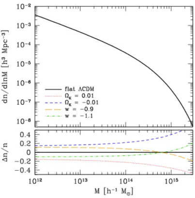
In Figure 1.6, we can see the predicted halo mass function for the standard Λ_{− CDM model and, in the bottom panel, the fractional changes induced} by adopting different cosmological models (Weinberg et al., 2013).

1.1.6 Cluster mass and cosmology

The cosmological model can be constrained using different and complemen-tary methods.

Type Ia supernovae (SN Ia) can be considered standard candles since they show a tight correlation between their peak luminosity and the shape of their light curves (Phillips, 1993). Comparing the peak apparent mag-nitude of distant SN to those of local (z < 0.1) calibrators with distances inferred from the distance scale ladder, we can measure the luminosity dis-tance DL(z), which is related to the cosmological parameters by Equations

1.1-1.4 (Weinberg et al., 2013).

CMB anisotropies can provide strong constraints on Ωm, Ωb and Ωk. In

fact, the amplitudes of the acoustic peaks in the CMB angular power spec-trum depend on the matter and baryon densities, while the locations of the peaks depend on spatial curvature (Weinberg et al., 2013).

The ratio between baryonic and total mass in massive galaxy clusters is expected to match the ratio of the cosmological parameters Ωb/Ωm. The

combination of X-ray gas mass fraction measurements in clusters with the determination of Ωb from CMB data can be used to put tighter constraints

(38)

Figure 1.6 – Halo mass function for the standard Λ − CDM model and fractional changes induced by varying the w and Ωk cosmological parameters