RETRIEVING RAIN RATES FROM SPACE BORNE MICROWAVE SENSORS USING U-NETS

HAL Id: insu-02894942

https://hal-insu.archives-ouvertes.fr/insu-02894942

Submitted on 9 Jul 2020

HAL is a multi-disciplinary open access archive for the deposit and dissemination of sci-entific research documents, whether they are pub-lished or not. The documents may come from teaching and research institutions in France or abroad, or from public or private research centers.

L’archive ouverte pluridisciplinaire HAL, est destinée au dépôt et à la diffusion de documents scientifiques de niveau recherche, publiés ou non, émanant des établissements d’enseignement et de recherche français ou étrangers, des laboratoires publics ou privés.

Copyright

RETRIEVING RAIN RATES FROM SPACE BORNE

MICROWAVE SENSORS USING U-NETS

Nicolas Viltard, Pierre Lepetit, Cécile Mallet, Laurent Barthès, Audrey

Martini

To cite this version:

Nicolas Viltard, Pierre Lepetit, Cécile Mallet, Laurent Barthès, Audrey Martini. RETRIEVING RAIN RATES FROM SPACE BORNE MICROWAVE SENSORS USING U-NETS. Climate Informatics 2020. 10th International Conference, Sep 2020, Oxford, United Kingdom. �insu-02894942�

RETRIEVING RAIN RATES FROM SPACE BORNE…

R

ETRIEVING

R

AIN RATES FROM SPACE BORNE

MICROWAVE SENSORS USING

U-

NETS

.

Nicolas Viltard, Pierre Lepetit, Cécile Mallet, Laurent Barthès, Audrey Martini

Université Paris-Saclay, UVSQ, CNRS, LATMOS, 78280, Guyancourt, France

Abstract— Despite a lot of progress over the last

decades, rain retrieval from spaceborne measurement has been a challenge since the first launch of a passive microwave radiometers on one of the NOAA Defense Meteorological satellites in the 70s. Deep-learning and convolutional U-Nets might be able to offer a breakthrough on the topic because they do take into account the topology of both the rain field and the measured brightness temperatures. The present paper offers the very first results on the application of such artificial neural networks on the rain retrieval problem.

I. MOT IV AT I O N

Retrieving rain rates at a global scale is a difficult problem because of the specifically intermittent nature of rain both spatially and temporally. Measurements of microwave brightness temperatures at various wavelength have been made almost continuously since the 70s but only in 1997 with the launch of the Tropical Rainfall Measuring Mission (TRMM, [1]) did this research field made substantial progresses. This first breakthrough was due to the combination on the same satellite of the Precipitation Radar (PR) and the TRMM Microwave Imager (TMI). Nowadays, the successor of TRMM, Global Precipitation Measurement (GPM, [2]) is a more ambitious project made of a mother satellite and a constellation of daughters. The mother satellite is very similar in design to TRMM with the GPM Microwave Imager (GMI) and the Dual-frequency Precipitation Radar (DPR), sharing part of their swath.

Radars are able to measure more directly the rain rate near the surface but for technical reasons, their swath is limited to about 200 km. Microwave radiometers offer a much broader swath (~1000 km) but their measurement of the rain is much more indirect. To overcome the latter problem, microwave radiometers perform a measurement at various channels ranging from 10 to 200 GHz and providing complementary

information. The brightness temperature measurements in the different channels can be treated as channels of a classical RGB image and the rain field seen by the radar can be considered as the target image to be retrieved. Although most operational rain retrieval algorithms are Bayesian-based ([3], [4]), the ability of artificial Neural Networks (NN) to approximate complex nonlinear functions have encourage their use in precipitation estimation from satellite. In [5], the authors trained a gated-expert network (GE) (a partition of the measurement space is automatically done with dedicated MLPs being adapted simultaneously on each subspace) on simulated brightness temperatures computed from atmospheric profiles obtained from a numerical weather prediction model (ECMWF) to retrieve RR from TMI observations. In [6], a segmentation of infrared geostationary satellite imagery is performed with a self-organized characteristic map. An empirical relationship between the brightness temperature and the precipitation is then calibrated for each of the clusters. Most of the preceding NN algorithms are based on fully connected neural network. Multi-layer perceptron (MLP) have been commonly used: in [7], the authors trained an MLP on the simulation performed with a numerical weather prediction model to retrieve RR from AMSU-B observations. In [8], the MLP was trained using collocated PR measurements to retrieve RR from SSM/I brightness temperatures observations, and in [9], as in our study, the MLP was trained with a database built from global GMI-DPR observations. Recently stacked denoising auto-encoder have been trained to automatically extract the features from infrared cloud images [10] or for the estimation of precipitation using bispectral satellite information, channels infrared (IR) and water vapor (WV) [11]. All the previous studies are based on a pixelwise approach. They therefore do not exploit potential information contained in the

relationships that may exist between the horizontal and vertical structures of precipitating events. The relationships between the microwave radiation of the atmosphere (Tb) and the rate precipitating at the surface (RR) are indeed very dependenton the structure of the precipitating systems.

Rain systems are also essentially 3-dimensionnal structures and the GMI and the DPR observe the same pixel under very different geometry. If the radar can be approximated as viewing “from above”, the GMI has a

50° incidence angle at surface which leads to a substantial parallax effect. This is amplified by the fact that the various channels of GMI are sensitive to different altitudes in the atmosphere and these altitudes depend on the atmospheric conditions themselves. This is likely one of the difficulties faced by the pixel-by-pixels retrieval techniques such as previous NN studies mentioned above, BRAIN [3] or Gprof [4] and why processing the brightness temperature scene as an image could be an advantage.

II. DA TA B AS E

GMI is a conically scanning radiometer with channels at 36.6 and 89 GHz. Channels are measured in both Horizontal (H) and Vertical (V) polarization. Additional channels at both lower and higher frequency are also available but were not used for the present test. All the pixels for each channel are co-located but each have a different spatial resolution depending on their respective

frequency: 15.6x9.4 km2 _{for the 36.6 GHz and 7.2x4.4}

km2 _{for 89 GHz. GMI swath is 904 km.}

DPR surface rain product results of the merged use of the Ka- (13.4 GHz) and Ku-band (35.5 GHz) radars. DPR provides 3D precipitation field with vertical resolution of 250 m, a horizontal resolution of 5 km, and swath widths of 245 km.

Data from the DPR are co-located spatially and temporally with the brightness temperatures from the GMI. A one-minute lag does exist between the radar and the radiometer observation of the same area but this is considered to be negligible at the considered spatial resolution. The co-location is performed by averaging the surface rain from the DPR pixels that fall within 5 km of a GMI pixel. All distances are computed using the latitude-longitude given for the center of each pixels which represent the center of the instruments’ beam at the Earth surface.

The target image is made of the DPR averaged surface rain rate (precipRateESurface) standard product found in 2A.GPM.DPR files. The rain rate is given in mm.hr-1 _{at the surface and has been converted}

from corrected radar reflectivity through a complex process beyond the scope of the present paper ([12] both GMI and DPR data are freely available at

https://storm.pps.eosdis.nasa.gov, after registration). Outside of the common swath between the two instruments there are no DPR data and the surface rain rate is set to a missing value (-9).

About 18 months of data from January 2017 to August 2018 were used to build the database. Each granule was split in 221x256 pixels images made of the four brightness temperature layers mentioned above and the target rain layer. Fig. 1 shows an example of such an image: three of the four input brightness temperature (TB) channels and the associated DPR surface rain rate

(RR) are presented. On the RR subplot, the green horizontal band represents the swath of the DPR while the whole height of the images represents the swath of GMI. It is to be noted that a slight yaw motion on the satellite during its orbital revolution changes the relative positions of the DPR and GMI swath by a few GMI pixels.

About 80,000 such 5-layer images are thus generated. Because natural rain occurrence is low, a lot of the images are actually without rain, so a selection is made based on the number of rainy pixels. Only the images with at least 100 pixels with rain > 0.1 mm.hr-1 _{or 10}

pixels > 100 mm.hr-1 _{are selected, resulting finally in}

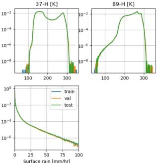
36440 images. The obtained data base is divided in 23,000 images for the training, 8,000 for the validation and 5440 for the test databases. Fig. 2 shows the

Figure 1: Three of the four input brightness temperatures ([K]) of GMI from an orbit on 2018-02-17 and the associated co-located surface rain rate ([mm.hr-1_{]) from DPR presented as}

histograms of each of the databases for two of the inputs: the TBs at 37 GHZ and 89 GHz both in horizontal

polarization and the target rain rate. This figure illustrates one of the difficulties in training arising from the distribution of rain intensities which is largely dominated by light rain and has a very scarce occurrence of heavy rain.

Figure 2: histograms of the three databases for two of the brightness temperatures 37 GHz-H (top left) and 89 GHz-H (top right) used as input and the rain rate used as target. Y-axis is the normalized frequency of occurrence.

It is to be noted that in addition to their swath difference, there is also a parallax effect between the two instruments. The DPR is basically a cross-track scanning instrument meaning that its sampling is performed in a plane perpendicular to the satellite motion on each side of the nadir point. The GMI is a conically-scanning instrument whose beam describes a circle at the Earth’s surface with a constant incidence angle of about 50°. Since the 89 GHz channels is mostly sensitive to scattering effects in the upper parts of the clouds, a spatial shift between the location of DPR’s maximum rain and GMI coldest brightness temperature can be observed even in the most structured convective events. This has been one of the reasons why such rain retrieval are extremely challenging.

III. MET H OD

Images from the training and validation database are cropped to 128x128 pixel sub-images randomly picked in the original. The they are also rotated randomly by

steps of 90° to prevent the network to learn just the position of the radar rain band.

A Full Convolutional Network of the U-net type is then used [13] under the PyTorch framework. The U-net is a combination of 3x3 convolutions, max-pooling and ReLU filters [13] that was adapted for the detection and restoration of clutter echoes in weather radar data [14]. Each layer of filtering down-samples the input images into what is called feature maps. The last feature map is then re-deployed using a series of transposed convolution layers. Concatenations (skip connections) between feature maps at various level of the filtering process allow to mix local and global information.

The initialization of the weights, the optimization method (Adam, [16]) and the learning rate (10-4_{) follow}

usual recommendation from literature [15]. The learning rate decreases by 0.5 every 100 epochs. During the training phase, the network’s parameters are upgraded through a gradient descent.

The loss function is set as the mean squared distance between the output rain and the target rain regardless of the rain intensity.

The network presented here results of a 600-epoch learning on the base described above.

IV. RES UL TS

Two example cases are given on Fig. 3 and 4. The first case is a frontal band over France observed on August 18th_{, 2018 which is a good prototype for land and coastal}

retrieval with moderately active isolated convection embedded in large stratiform areas.

The second case is typhoon Harold observed on April 6th_{, 2020 which is a good case of intense convective rain}

over ocean.

As a comparison, the results from the last publicly available version of the Gprof algorithm [4] are presented. Gprof is the current GPM operational product, based on a Bayesian approach to perform the retrieval.This algorithm is a reference in the community in terms of rain retrieval and uses auxiliary data to constrain the solutions (temperature, surface type, humidity, cloud cover…).

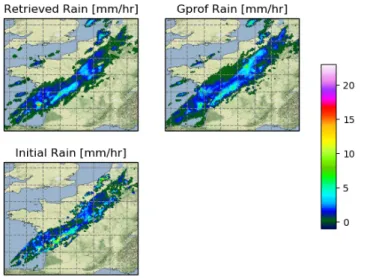
Figure 3: comparison between the initial (bottom, DPR) surface rain, the retrieved (top left) and the Gprof surface rain for a weak frontal band on 18th of August 2018.

In both situations, the algorithm performs very well in terms of rain/no-rain detection with a 0.1 mm.hr-1

threshold applied. This threshold is meant to filter out some remaining noise in the output. The handling of coastal areas which is usually extremely difficult seems to be very smooth. Islands and coastlines are not covered with rainy pixels and rain over coast does not show apparent or marked discontinuities.

For these two cases, the performances are compared with Gprof. The bias for the frontal case is about 0.16 mm.hr-1 _{(Mean Absolute Error: 1.08 mm.hr}-1_{) for Gprof}

and 0.20 mm.hr-1 _{(MAE: 0.85 mm.hr}-1_{) for our}

algorithm. Similarly, for the typhoon case, the bias is 0.58 mm.hr-1 _{(MAE: 1.79 mm.hr}-1_{) for Gprof and 0.25}

mm.hr-1 _{(MAE: 1.40 mm.hr}-1_{) for our algorithm. On}

these two examples, the Deep-Learning algorithm seems to perform slightly better. For the more convective situation of Harold, the difference is clearer. For the frontal situation, Gprof has a better bias but it seems to be due to some compensating effects because the MAE is not as good as the Deep-Learning algorithm. The test dataset presented in section II is then used to assess the algorithm’s performances. As for the two cases study, a 0.1 mm.hr-1 _{threshold is applied for}

rain/no-rain discrimination and after application of this threshold, 4976334 pixels are flagged as rainy in the test dataset. Taking the DPR surface rain as the reference, the results are summarized in Table 1. The rain/no-rain detection rate is very good and only the “bad detection” situations are slightly high meaning that the algorithm tends to miss rain when the DPR does not.

Figure 4: Same as Fig 3 but for surface rain for Typhoon Harold on 6th April 2020.

It is to be noted that 0.1 mm.hr-1 _{is a rain intensity that}

is at the edge of detectability for instantaneous rain estimates whichever measurement system is considered. Fig. 6 shows the bias as a function of the pixel position in the common swath between the two instruments. It can be seen that this error is actually very small and consistent throughout but it is also structured with a slight degradation of performances at the center. This latter degradation is under investigation.

Table 1: The numbers are computed with a threshold of 0.1 mm/hr.

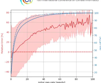
Fig. 7 shows relative error ((initial – retrieved)/initial) as a function of the initial (DPR) rain rate. There is a slight overestimation of the light rain rates below 5 mm.hr-1 _{but with a fairly large standard deviation. Then,}

as expected, the bias increases with rain intensity because the retrieved rain tends to underestimate the rain as it becomes more intense. At the same time, the relative error standard deviation diminishes as the rain rate increases. This is a very classical result which is likely due the decorrelation of the surface rain intensity

BIAS [mm.hr-1_{] (%)} FRACTION GOOD DETECTION -0.065 83.7 FALSE ALARM 0.198 3.13 BAD DETECTION -0.185 16.6 NO RAIN 0.005 96.8

and the used brightness temperatures which are mainly sensitive to the ice layer aloft. The two cumulative distribution of rain are close but, as expected, the retrieved rain rates at the highest end of the spectrum are re-distributed in the 10 to 40 mm.hr-1 _range.

Figure 5: training and validation losses evolution as a function of the number of epochs.

Fig. 8 shows the frequency distribution of both the initial and the retrieved rain as a function of initial rain intensity. Up to 20 mm.hr-1_{, the agreement is excellent}

and then the two distributions slowly drift apart. One can see here the difficulty to learn properly to retrieve the higher rain rates because of their scarcity in the training dataset. The difference in the distribution between Fig. 8 and Fig. 2 comes from the 0.1 mm.hr-1

threshold used in the retrieved rain.

Figure 6: The blue solid line is the bias computed as initial rain minus retrieved rain as a function of pixel position in the common swath for initial rain > 0.1 mm.hr-1_{(the center of both}

instrument’s swath is approximately rank 100). Shades of red are for the standard deviation. The orange solid line is the average rain per pixel position in the DPR scan.

Figure 7: relative error (initial – retrieved) per class (red, left hand-side y-scale) as a function of initial (DPR) rain intensity and associated standard deviation in shade of red. Right hand-side y-axis (blue) is the cumulative distribution of surface rain for initial (blue solid) and retrieved (blue dashed).

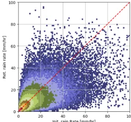
Fig. 9 shows that this good agreement is mostly due to a balance between under and over-estimated pixels. Above 30 mm.hr-1 _{the underestimation becomes more}

visible and it can be seen that rain intensities above 80 mm.hr-1_{are quite rare in the retrieved rain.}

Figure 8: pdf of initial (DPR) and retrieved rain as a function of initial rain intensity on the test database (with a 0.1 mm.hr-1 threshold for rain/no-rain).

A more thorough comparison of our results and those of Gprof versus the DPR surface rain was performed for two distinct months: December 2018 and May 2020. These two months were chosen because on the one hand they are characteristic of opposite Winter and Summer seasons and on the other hand 2020 was further in time from the learning database. All the orbits (~500/month) of GMI, DPR and the Gprof outputs were co-located for

the two months. The results were then averaged over 2°x2° boxes in order to see how the differences between DPR and the radiometric-based retrievals were spatially and temporally structured.

It is to be noted that if our algorithm has learned to retrieve the surface rain rate from DPR, the Gprof algorithm is based on slightly different principles and it is designed to converge toward the DPR estimates but not to be exactly equal to it. Thus, it is no surprise that our U-net algorithm gets better results when compared to DPR.

No significant difference in terms of errors intensities and structures were found between December 2018 and May 2020, so Fig. 10 and the errors are only given for the results averaged over the two months together. This is a very positive point because it means that the network has not learned to retrieve the rain of 2017 and 2018 and to retrieved indeed the rain in general.

The first striking feature on Fig. 10 is the performance difference between land and ocean for Gprof. If the U-Net seems to perform very homogeneously over land and ocean, Gprof provides higher estimates over land than DPR. Over ocean, the two algorithms offer very similar patterns in terms of difference with DPR.

In terms of average difference and at this 2°x2° spatial resolution, Gprof is 0.17 mm.hr-1 _{above DPR (with a}

standard deviation of 0.45 mm.hr-1 _{and a MAE of 0.29}

mm.hr-1_{) while the U-net algorithm is 0.03 mm.hr}-1

above DPR (with a standard deviation of 0.34 mm.hr-1

with a MAE of 0.19 mm.hr-1_{). As an indication, the}

mean DPR surface rain rates for these two months is 1.09 mm.hr-1_.

V. CON C LU S IO NS

This is a first test on the use of Deep-Learning techniques and more specifically a U-net to retrieve rain from brightness temperatures. The dataset is made of co-located data from the GPM Microwave Imager and the GPM Dual-frequency Precipitation Radar. Only the two 36.6 GHz and the two 89 GHz channels were used as input. These four channels are mostly sensitive to ice scattering so their correlation to surface rain is only statistical, through convective activity. But these channels are also the channels with the highest spatial resolution, most compatible with the high spatial variability of rain itself.

The paradigm of this first test was to use no auxiliary information in order to assess purely the effect of treating the brightness temperature scenes as images. Most retrieval algorithms work pixel-by-pixel and take

almost no account of the environment of the other pixels.

The developed network performs well when compared with Gprof which is the reference algorithm in the GPM community. Our network offers an overall low bias, similar performances on land, coast and ocean and a good handling of the transitions between each of these surface types, without a priori information. The rain/no-rain detection is excellent when assuming a threshold of 0.1 mm.hr-1_{. Performances in situation of convection}

seem slightly better as expected when using 37 and 89 GHz channels because of the better correlation between rain intensity and ice content in active convection. The network seems nonetheless to be able to maintain performances in a stratiform environment.

Figure 9: 2-D histogram of the retrieved rain vs. initial (DPR) rain, color indicates density of points.

To go further, a more detailed study of the error structure will be necessary in the future. Balancing the learning bases and modifying the loss function will also be necessary in order to try to improve the retrieval of the higher rain rates knowing however that the information might not be present “as is” in the brightness temperature data due to some sort of “saturation” in the scattering signature. Finally, addition of auxiliary data (e. g. latitude, longitude, local temperature and/or local humidity) and both extra GMI channels and the use of different DPR rain layer will be tested in the future. Generalisation to other passive microwave radiometers will also be attempted.

Figure 10: 2°x2° averaged difference between top: DPR - U-net retrieved rain and bottom DPR - Gprof retrieved rain. The averages are performed over all the orbits of December 2018

and May 2020.

ACK NOW LE D GM E NT S

This research is work is supported by a Centre

National d’Etudes Spatiales (CNES) grant.

REF ER EN CE S

[1] C. Kummerow, W. Barnes, T. Kozu, J. Shiue, J. Simpson, 1998: The Tropical Rainfall Measuring Mission (TRMM) Sensor Package. J. of Atmos. and Ocean. Technol. Vol. 15, no. 3, pp. 809–817.

[2] E. A. Smith, G. Asrar, Y. Furuhama, A. Ginati, C. Kummerow, V. Levizzani, A. Mugnai, K. Nakamura, R. Adler, V. Casse, M. Cleave, M. Debois, and J. Durning, 2007: International Global Precipitation Measurement (GPM) Program and Mission: An Overview. Springer -

Measuring Precipitation from Space - EURAINSAT and the future. Vol. 28, pp. 611-653.

[3] N. Viltard, C. Burlaud and C. D. Kummerow, 2006: Rain retrieval from TMI brightness temperature measurements using a TRMM PR–based database. J. Appl. Meteor.

Climatol., 45, 455–466

[4] C. D. Kummerow, D.L. Randel, M. Kulie, N. Wang, R. Ferraro, S. Joseph Munchak, and V. Petkovic, 2015: The Evolution of the Goddard Profiling Algorithm to a Fully Parametric Scheme. J. Atmos. Oceanic Technol., 32, 2265–2280

[5] E. Moreau, Mallet C., Thiria S., Mabboux X., Badran F., Klapisz C., 2002: Atmospheric Liquid Water Retrieval Using a Gated Expert Neural Network, J. of Atmos. and

Ocean. Tech., 19, 457-466

[6] Y. Hong, K. Hsu, S. Sorooshian and X. Gao, 2004: Precipitation Estimation from Remotely Sensed Imagery Using an Artificial Neural Network Cloud Classification System. J. of Appl. Meteor., 43, 1834-1853

[7] C. Surussavadee and D. H. Staelin, 2208: Global Millimeter-Wave Precipitation Retrievals Trained With a Cloud-Resolving Numerical Weather Prediction Model, Part I: Retrieval Design. IEEE Transactions on Geosci.

and R. Sens., 46, 99-108

[8] C. Mahesh, S. Prakash, V. Sathiyamoorthy, R.M. Gairola, 2011: Artificial neural network based microwave precipitation estimation using scattering index and polarization corrected temperature. Atmos. Res., 102, 358-364

[9] P. Sanò G. Panegrossi, D. Casella, A.C. Marra, L.P. D’Adderio, J.F. Rysman and S. Dietrich, 2018: The Passive Microwave Neural Network Precipitation Retrieval (PNPR) Algorithm for the CONICAL Scanning Global Microwave Imager (GMI) Radiometer. Remote

Sens. 10, 1122

[10] Y. Tao, X. Gao, A. Ihler, K. Hsu and S. Sorooshian, 2016: Deep neural networks for precipitation estimation from remotely sensed information. 2016 IEEE Congress on

Evol. Comp. (CEC), Vancouver, BC, 1349-1355

[11] Y. Tao, X. Gao, A. Ihler, S. Sorooshian and K. Hsu, 2017: Precipitation identification with bispectral satellite information using deep learning approaches.J. of

Hydrometeor.,18, 1271-1283.

[12] N. B. Adhikar., T. Iguchi, S. Shinta et al., 2007: Rain retrieval performance of a dual-frequency precipitation radar technique with differential-attenuation constraint. IEEE Trans. Geo. and Rem. Sens., Vol. 45, pp. 2612-2618.

[13] O. Ronneberger, P. Fischer,and T. Brox, 2015: U-net: Convolutional networks for biomedical image segmentation. Int. Conf. on Med. Image Comput. and

Computer-Assisted Interv. Springer, pp. 234–241.

[14] P. Le Petit, L. Barthès, C. Mallet, C. Ly, N. Viltard, Y. Lemaître, 2020: Using Deep Leaning for Restoration of Precipitation Echoes in Radar Data, IEEE Transac.

Gesosci. And R. Sensing. Conditionally accepted.

[15] X. Glorot and Y. Bengio, 2010: Understanding the difficulty of training deep feedforward neural networks.

Proc. 13th _{Int. Conf. on Artificial Intelligence and}

Statistics, pp 249-256

[16] P. D. Kingma and J. Ba, 2014: Adam: A method for stochastic optimization. arXiv preprint arXiv:1412.6980