HAL Id: hal-02401070
https://hal.parisnanterre.fr//hal-02401070
Submitted on 5 Jan 2021
HAL is a multi-disciplinary open access
archive for the deposit and dissemination of
sci-entific research documents, whether they are
pub-lished or not. The documents may come from
teaching and research institutions in France or
abroad, or from public or private research centers.
L’archive ouverte pluridisciplinaire HAL, est
destinée au dépôt et à la diffusion de documents
scientifiques de niveau recherche, publiés ou non,
émanant des établissements d’enseignement et de
recherche français ou étrangers, des laboratoires
publics ou privés.
A new assessment of the solar s- and r- process
components
N. Prantzos, C. Abia, S. Cristallo, M Limongi, A Chieffi
To cite this version:
N. Prantzos, C. Abia, S. Cristallo, M Limongi, A Chieffi. Chemical evolution with rotating massive
star yields II. A new assessment of the solar s- and r- process components. Monthly Notices of the
Royal Astronomical Society, Oxford University Press (OUP): Policy P - Oxford Open Option A, 2019,
�10.1093/mnras/stz3154�. �hal-02401070�
arXiv:1911.02545v1 [astro-ph.GA] 6 Nov 2019
Chemical evolution with rotating massive star yields
II. A new assessment of the solar s- and r- process
components
N. Prantzos,
1
⋆
C. Abia,
2
S. Cristallo
3,4
M. Limongi,
5,6
A. Chieffi
7,8
1Institut d’Astrophysique de Paris, UMR7095 CNRS, Sorbonne Universit´e, 98bis Bd. Arago, 75104 Paris, France 2Departmento de F´ısica Te´orica y del Cosmos, Universidad de Granada, E-18071 Granada, Spain
3 Istituto Nazionale di Astrofisica - Osservatorio Astronomico d’Abruzzo, Via Maggini snc, I-64100, Teramo, Italy 4 Istituto Nazionale di Fisica Nucleare - Sezione di Perugia, Via Pascoli, I-06123, Perugia, Italy
5 Istituto Nazionale di Astrofisica - Osservatorio Astronomico di Roma, Via Frascati 33, I-00040, Monteporzio Catone, Italy 6 Kavli Institute for the Physics and Mathematics of the Universe, Todai Institutes for Advanced Study, the University of Tokyo,
Kashiwa, Japan 277-8583 (Kavli IPMU, WPI)
7 Istituto di Astrofisica e Planetologia Spaziali, INAF, via Fosso del cavaliere 100, 00133 Roma - Italy
8 Monash Centre for Astrophysics (MoCA), School of Mathematical Sciences, Monash University, Victoria 3800, Australia
Accepted XXX. Received YYY; in original form ZZZ
ABSTRACT
The decomposition of the Solar system abundances of heavy isotopes into their s-and r- components plays a key role in our understs-anding of the corresponding nuclear processes and the physics and evolution of their astrophysical sites. We present a new method for determining the s- and r- components of the Solar system abundances, fully consistent with our current understanding of stellar nucleosynthesis and galac-tic chemical evolution. The method is based on a study of the evolution of the solar neighborhood with a state-of-the-art 1-zone model, using recent yields of low and in-termediate mass stars as well as of massive rotating stars. We compare our results with previous studies and we provide tables with the isotopic and elemental contributions of the s- and r-processes to the Solar system composition.
Key words: Galaxy: abundances – Galaxy: evolution – Nucleosynthesis – Sun:
abun-dances – Stars: abunabun-dances
1 INTRODUCTION
In their compilation and analysis of Solar system isotopic abundances Suess & Urey (1956) were the first to notice that, if heavier than Fe nuclei are formed by successive cap-ture of neutrons, one should expect two abundance peaks for each of the regions near magic neutron numbers: a sharp one at the position of the magic nucleus, from material pilled up there due to the low neutron capture cross-section when neutron captures take place near the β-stability valley; and a smoothed one at a few mass units below, from material made by neutron captures occurring in the neutron-rich side of the stability valley and radioactively decaying after the end of the process.
Building on that compilation, Burbidge et al. (1957) worked out the details of the two nucleosynthetic processes, which they called s- and r-, respectively1. The former (slow)
⋆ E-mail: [email protected]
1 There are observational indications of intermediate density
would occur on timescales long with respect to the life-times of radioactive nuclei along the neutron path, i.e. tens to thousands of years, as a result of low neutron densities Nn∼106÷107 cm−3. The latter (rapid) would take place on
short timescales of the order of 1 s, as a result of high neutron densities Nn>1024cm−3.Burbidge et al.(1957) also noticed
that, along the s- process path (i.e. the valley of nuclear sta-bility), the product of the neutron capture cross-section σA
and the abundance NAof a nucleus with mass number A> 70
is a smooth function of A, first declining up to A∼100 and then levelling off up to A= 208. They attributed that feature to the operation of the s-process in two different regimes, the former one having ”not enough neutrons available per56Fe
neutron capture processes (i.e. between the s- and r- process), like the i- process (Cowan & Rose 1977; Dardelet et al. 2014;
Hampel et al. 2016), possibly occurring in rapidly accreting white dwarfs (Denissenkov et al. 2017), proton ingestion episodes in low-metallicity low-mass asymptotic giant branch (AGB) stars (Cristallo et al. 2016) or super-AGB stars (Jones et al. 2016).
nucleus to build the nuclei to their saturation abundances”, while the constancy of σANAin the latter is ”strongly
sug-gestive of steady flow being achieved and of all of the nuclei reaching their saturation abundances”.
Following the work ofWeigert(1966), the environment provided by low and intermediate mass stars (LIMS) on their AGB phase was identified bySchwarzschild & H¨arm(1967) and Sanders (1967) as a promising site for the operation of the s-process. Today, those stars are thought to produce the bulk of the s-isotopes above A∼ 90 during their thermal pulses, with neutrons released mainly by the 13C(α,n)16O
reaction (see Straniero et al. 1995; Gallino et al. 1998 and references therein). On the other hand, Peters (1968) sug-gested that in the He-burning cores of massive stars, neu-trons released by the 22Ne(α,n)25Mg reaction should also
produce s-nuclei. Today, those stars are thought to pro-duce the s-nuclei in the regime of ”few neutrons per 56Fe
seed”, i.e. below A∼ 90 (Couch et al. 1974;Lamb et al. 1977;
Busso & Gallino 1985): stellar models - including those of
Prantzos et al. (1987) with mass loss - show that despite the large abundance of 22Ne, most of the released
neu-trons are captured by its progeny 25Mg and other abun-dant nuclei, leaving few neutrons to be captured by 56Fe
(see Prantzos et al. 1990, for details of the ”neutron econ-omy trio”, i.e. the roles of neutron sources, seed and poisons as function of metallicity in the case of massive stars). In con-trast, in the thermally pulsing phase of AGBs, the periodic mixing of protons in the He-layer maintains the13C source to
a high abundance level - through12C(p,γ)13C - and releases
sufficient neutrons to reach the ”saturation regime”. Thus, both the mechanism(s) and site(s) of the s- process are con-sidered to be sufficiently well known (see e.g.K¨appeler et al. 2011, and references therein).
On the other hand, the situation with the site of the r-process is still unsatisfactory. After more than fifty years of research on its astrophysical origin(s), the identification of a fully convincing site remains still elusive. An exhaustive description and discussion of experimental, observational and theoretical aspects of the r-process, as well as on the sites so far proposed is provided in the recent reviews of
Cowan et al.(2019) andThielemann et al.(2017). However, up to date, no numerical simulation in the proposed scenar-ios has been able to fully reproduce the observed distribu-tion of the r-process elemental and isotopic abundances in the Solar system. Nowadays the neutron star merging (NSM) scenario is given support by the recent joint detection of elec-tromagnetic and gravitational signal from the γ−ray burst GW170817/GRB170817A (see Pian et al. 2017, and refer-ences therein), and, in particular, by the identification of the neutron-capture element Sr in the spectrum of the asso-ciated kilonova AT2017gfo (Watson et al. 2019). However, it is not yet completely understood which component of those systems (dynamical, disk, ν-wind) dominates the nucleosyn-thesis, since any one of them may cover a wide range of chem-ical distributions, depending on the adopted input param-eters (Rosswog 2015;Fern´andez & Metzger 2016;Wu et al. 2016;Perego et al. 2017). An additional important source of uncertainty comes from the nuclear inputs adopted to calcu-late the r-process nucleosynthesis, the most important ones being nuclear masses, β-decay rates and nuclear fission mod-els (Eichler et al. 2015;Thielemann et al. 2017). Finally, the observed evolution of the r-elements in the Galaxy is hard
(albeit not impossible) to conciliate with our current under-standing of the occurrence rate of NSMs, regarding both the early (halo) and the late (disk) phases of the Milky Way (Tsujimoto & Shigeyama 2014; Ishimaru et al. 2015;
Ojima et al. 2018;Cˆot´e et al. 2018;Hotokezaka et al. 2018;
Cˆot´e et al. 2018;Guiglion et al. 2018;Wehmeyer et al. 2019;
Siegel et al. 2019; Haynes & Kobayashi 2019; Cˆot´e et al. 2019).
The decomposition of the Solar system abundances of heavy elements into their s- and r- components, played and will continue to play a pivotal role in our understanding of the underlying nuclear processes and the physics and evo-lution of the corresponding sites. The s-contribution can be more easily determined, since isotopes dominated by the s-process form close the β−stability valley. Their nuclear prop-erties (β−decay half-times, nuclear cross sections, etc.) are more easily measured, while the astrophysical sites are bet-ter understood today. On the other hand, due to the large astrophysics and nuclear physics uncertainties related with the r-process, its contribution to the isotopic solar abun-dances has been so far deduced by a simple subtraction of the s-process contribution from the observed solar value.
In this work, we present a new method for determin-ing the s- and r-components of the Solar system abun-dances. It is based on a global study of the evolution of the solar neighborhood with a state-of-the-art 1-zone model of galactic chemical evolution (GCE), which is pre-sented in detail in Prantzos et al. (2018) - Paper I here-after - and adopts recent stellar yields of rotating massive stars (fromLimongi & Chieffi 2018) and of LIM stars (from
Cristallo et al. 2015a).
The plan of the paper is as follows: In §2, we review the various methods used so far in order to derive the s-component of the isotopic abundances of the heavy nuclei, and we discuss their shortcomings. In §3, we present in de-tail our new method and its assumptions. In §4we present our results. We compare first the isotopic contributions to previous studies (§4.1) , as well as to the measured Solar system abundances taking into account the uncertainties of the latter (§4.3). We discuss the resulting σANA curve in
§4.2 and we derive the r-residuals in §4.4. In §4.5 we de-rive the elemental s- and r-components, and finally in §5we summarized the main results of this study.
2 DETERMINATION OF S- AND R-ABUNDANCES
The ”classical” (or ”canonical”) s-process model was orig-inally proposed by Burbidge et al. (1957) and developed by Clayton & Rassbach (1967). In this model two main assumptions are made: a) the s-process temperature is constant, allowing one to adopt well determined neutron-capture cross sections; b) nuclei on the s-process path are either stable (τβ>> τn) or sufficiently short-lived that the
neutron capture chain continues with the daughter nucleus (τβ << τn). This second assumption, however, is not valid
at the s-process branchings (τβ∼τn), which requires a
spe-cial treatment (see e.g.Kappeler et al. 1989). In addition, the classical model assumes that some stellar material com-posed by iron nuclei only is excom-posed to the superposition of 3 exponential distributions of the time-integrated neutron
exposure, defined as τo=RotNnvTdt(where vT is the thermal
neutron velocity at the temperature T). The 3 exponential distributions are usually referred to as the ”weak” compo-nent (responsible of the production of the 70 6 A 6 90 s-nuclei), the ”main” component (for the 90 6 A 6 204 isotopes) and the ”strong component” (for A > 204). For long-enough exposures, the equations governing the evolution of the s-nuclei abundances result in equilibrium between the produc-tion and destrucproduc-tion terms, leading to a constant product, σANA, of neutron cross section and s-process abundance.
Al-though this condition is not completely reached, the prod-uct σANAshows a very smooth dependence on mass number
(see, e.g., Clayton 1968). Therefore, the product σANA for
a given isotope is fully determined by the cross section, af-ter the parameaf-ters τoand the number of neutrons captured
per 56Fe seed nucleus are fixed. The goal of the classical
approach is to fix the empirical σANA values for the s-only
isotopes, i.e. nuclei that are shielded against the r-process by the corresponding stable isobar with charge Z − 1 or Z − 2 (see §3.1for a discussion about our selection of s-only iso-topes). Once the Solar system s-only distribution is fitted, the s-contribution for the rest of the ”mixed” isotopes (with both a s- and r-contribution) are automatically obtained. Finally, the r-contribution is derived just subtracting this s-contribution Ns,A from the measured total Solar system
abundance NA. This classical method has been used
fre-quently in the literature, providing satisfactory results as the measurement of neutron cross sections have been improving during the years (see e.g.Kappeler et al. 1989;Sneden et al. 2008;K¨appeler et al. 2011).
However, the classical model is affected not only by ob-servational and nuclear input data uncertainties, but also by the assumption that the s-process operates at a fixed con-stant temperature and neutron and electron density, and by the hypothesis that the irradiation can be considered as exponential one. To test the influence of these assump-tions, Goriely (1999) (see also Arnould et al. 2007) devel-oped the so-called ”multi-event” s-process, which constitutes a step forward in the canonical method. The multi-event approach assumes a superposition of a number of canon-ical events taken place in different thermodynamic condi-tions, namely: a temperature range 1.5 6 T(K)/10864,
neu-tron densities 7.5 6 log Nn(cm−3) 6 10and a unique electron
density Ne= 1027 cm−3. Each canonical event is character-ized by a given neutron irradiation on the56Fe seed nuclei
during a given time at a constant temperature and neutron density. These conditions try to mimic the astrophysical con-ditions characterizing the site of the s-process, although it is well known that temperature and neutron density are not constant during the s-process (see e.g.K¨appeler et al. 2011, and references therein). The s-only nuclei abundance distri-bution obtained with that method is remarkably close to the solar observed one, because of the minimization proce-dure adopted in the selection of the aforementioned parame-ters. However, it presents non-negligible deviations from the classical method in the regions A 6 90 and A> 204, mainly because the resulting neutron exposures in the multi-event model clearly deviate from exponentials. Within the multi-event model it was possible to evaluate the major uncer-tainties (both nuclear and due to abundance measurements) affecting the prediction of the s-(r-)abundance distribution.
Goriely (1999) concluded that the uncertainties in the
ob-served meteoritic abundances and the relevant (n, γ) rates have a significant impact on the predicted s-component of the solar abundance and, consequently, on the derived r-abundances, especially concerning the s-dominated nuclei (see alsoNishimura et al. 2017andCescutti et al. 2018).
Stellar models of LIM stars during the AGB phase and of massive stars during hydrostatic core He-burning and shell C-burning (the two widely recognized sites of the s-process), have shown that the interplay of the different thermal conditions for the13C and22Ne neutron sources is
hardly represented by a single set of effective parameters constant in time (Busso et al. 1999; Straniero et al. 2006;
Limongi & Chieffi 2018), such as those used in the classical (or the multi-event) approach. In an effort to overcome this shortcoming, the results of the ”stellar” model have been used to estimate the contributions of the s- and r-process to the Solar system abundances. This method is based on post-processing nucleosynthesis calculation performed in the framework of ”realistic” stellar models. The first attempt to apply this method was made byGallino et al. (1998) and
Arlandini et al.(1999), and more recently byBisterzo et al.
(2010) with updated nuclear input. These authors showed that the solar s-process main component can be reasonably reproduced by a post-processing calculation from a particu-lar choice (mass and extension) of the13C pocket (the main
neutron source in AGB stars) by averaging the results of stellar AGB models (Gallino et al. 1998) between 1.5 and 3 M⊙ with [Fe/H]∼ −0.3. This model is particularly
success-ful in reproducing the s-only nuclei solar abundances and showed general improvements with respect to the classical method, especially in the mass region A < 88 (Arlandini et al. 1999). In fact, all these nuclei (mainly produced by the weak s-component) are synthesized in much smaller quantities. This difference is caused by the very high neutron exposures reached in the stellar model, which favor the production of heavier elements. In particular, at the s-termination path,
208Pb is produced four times more than in the classical
ap-proach. Nevertheless, the stellar model used to derive the physical inputs of post-process calculations are affected by several theoretical uncertainties. One of the less constrained physical mechanisms is the one leading to the formation of the 13C pocket, which forms at the base of the
convec-tive envelope after each TDU episode. Different processes have been proposed as responsible of the formation of such a pocket: convective overshoot (Herwig et al. 1997), grav-ity waves (Denissenkov & Tout 2003; Battino et al. 2016), opacity induced overshootCristallo et al.(2009) and mixing induced by magnetic mixing (Trippella et al. 2016). Other critical quantities are the mass fraction dredged-up after each thermal instability (third dredge up, TDU) during the AGB phase, and the mass-loss rate. Actually, the two pro-cesses are degenerate, since the number (and the efficiency) of TDUs is determined by the mass of the H-exhausted core and of the H-rich convective envelope, which in turn depend on the adopted mass-loss rate. However, AGB stellar models show that an asymptotic s-process distribution is reached after a limited number of pulses, so the mass-loss uncer-tainty mainly affects the total yield of the s-processed mate-rial, and not so much the shape of the resulting distribution (see e.g. Fig. 12 in Cristallo et al. 2015b). In the ”stellar” model, the r-residuals are calculated subtracting the arith-metic average of the 1.5 and 3 M⊙models at [Fe/H]∼ −0.3
(Z ∼ 1/2Z⊙)2 best reproducing the main s-component to the
observed solar abundances. InArlandini et al.(1999) the s-and r-components obtained by the stellar model method are compared to the classical one for nuclei A > 88, together with the corresponding uncertainty determined from the cross sections and solar abundances. Uncertainties in the s- and r-residuals coming from the stellar model itself are, however, difficult to estimate.
The massive star contribution to the solar s- only com-position has been explored with non-rotating stellar mod-els in e.g. Prantzos et al. (1990); Raiteri et al. (1993) and more recently, with rotating massive stars inPignatari et al.
(2008); Frischknecht et al. (2016); Choplin et al. (2017,
2018); Limongi & Chieffi (2018). Such models have their own uncertainties (mass loss, mixing, nuclear etc.). The role of rotation, in particular, is poorly explored and understood at present. The main reason is that the rotation driven in-stabilities are included in a parametric way, and this means that the efficiency with which fresh protons are ingested in the He-burning zone is not based on first principles but it is determined by two free parameters that must be calibrated. The calibration adopted in the models adopted in this paper is discussed in detail inLimongi & Chieffi(2018). Moreover, since the proton ingestion scales directly with the initial ro-tational velocity (and hence the neutron flux as well), the adopted initial distribution of rotational velocities (IDROV) plays a pivotal role: already in Paper I we have shown that at least the average rotational velocity of the stars must be limited to < 50 km/s at metallicities [Fe/H]> −1, in order to avoid an overproduction of heavy nuclei, mainly in the Ba peak. But there are also other subtle indirect factors that may change the yields predicted by rotating models: in order to bring protons in an He active environment, at least part of the H rich mantle must be present while He is burning. A substantial change in the mass loss rate (e.g. due to the inclusion of a dust driven component to the mass loss rate or to the overcome of the Eddington luminosity) may affect the range of masses that retain a substantial fraction of the H rich mantle while the stars are in the central He-burning phase.
Uncertainties of stellar models is one of the reasons why the validity of the stellar method has been questioned (see e.g.Arnould et al. 2007). Another one is that this method does not consider the solar s-(r-)process abundance distri-bution in an astrophysical framework, i.e. as the result of all the previous generations of stars which polluted the inter-stellar medium prior to the formation of the Solar system. In particular, these generations of stars covered a large range of metallicities and not a unique value (or even a limited range of values) of [Fe/H] as it is assumed in the classical and stellar methods. For instance, it is well known that at low metallicities a large neutron/seed ratio is obtained, lead-ing to the production of the heaviest s-nuclei, while at high metallicities the opposite happens (see e.g. Travaglio et al. 2004, and references therein).
The Solar system s-(r-) process abundances have to be understood in the framework of a galactic chemical
evolu-2 We adopt here the usual notation [X/H]= log (X/H) ⋆− log (X/H)⊙, where (X/H)⋆ is the abundance by number of the el-ement X in the corresponding object.
tion (GCE) model. This is certainly a difficult task that requires a good understanding of the star formation history in the Galaxy, of stellar evolution, and of the interplay be-tween stars and the interstellar gas, among other things. We are still far from fully understanding these issues. There-fore, this third method is based on a necessarily schematic description of the situation considering the chemical evolu-tion of our Galaxy, accounting for the fact that the site(s) of the r-process have not been clearly identified yet. Attempts to obtain the s- and r- components of the solar composi-tion from a GCE model were pioneered byTravaglio et al.
(2004), later updated bySerminato et al.(2009) and more recently byBisterzo et al.(2014,2017). These authors em-ployed a GCE code adopting s-process yields from AGB stel-lar models byGallino et al.(1998) in a range of masses and metallicities (see these papers for details). Regarding the r-process yields, and for elements from Ba to Pb, they esti-mated the contribution to the Solar system by subtracting the s-residuals from the solar abundances. Then, they scale the r-process yields to the yield of a primary element (in a similar way we do here, see Eq. 4) mainly produced in core collapse supernovae, which they assumed to occur in the mass range 8 − 10 M⊙. They derived the weak s-process
con-tribution fromRaiteri et al.(1993). On the other hand, for the lighter elements, in particular for Sr-Y-Zr, they deduced the r-residuals and, thus, the r-process yields, from the abun-dance pattern found in CS 22892-052 (Sneden et al. 2002), by assuming that the abundance signatures of this star is of pure r-process origin (i.e., any contamination by other pos-sible stellar sources is hidden by the r-process abundances). TheBisterzo et al.(2014) model resulted in good agree-ment with the Solar s-only isotopic abundances between
134,136Ba and204Pb, also showing that the solar abundance
of208Pb is well reproduced by metal-poor AGB stars,
with-out requiring the existence of a ”strong” component in the s-process as is done in the classical method. Below the magic number N = 82, however, they found a significant dis-crepancy between the abundance distribution obtained with their GCE model and the Solar system values. It turned out that their GCE model underproduces the solar s-process component of the abundances of Sr, Y and Zr by ∼ 20%− 30% and also the s-only isotopes from 96Mo up to 130Xe. This
result promptedTravaglio et al.(2004) to postulate the ex-istence of another source of neutron-capture nucleosynthesis named the light element primary process (LEPP). They ar-gued that this process is different from the s-process in AGB stars and also different from the weak s-process component occurring in massive stars. The recent updates of this study byBisterzo et al.(2014,2017), reach the same conclusion3.
In particular, these two studies ascribe a fraction ranging from 8% to 18% of the solar Sr, Y and Zr abundances to this LEPP, and suggest that lighter elements from Cu to Kr could be also affected. On the other hand, they obtained a
3 Bisterzo et al.(2014,2017) mainly focus on the impact of the different 13C pocket choices in AGB stars and weak s-process yields from massive stars, on the s-process residuals at the epoch of the Solar System formation. In Bisterzo et al.(2017) yields from massive stars are included considering the impact of rotation in a limited range of masses and metallicities according to the models byFrischknecht et al.(2016).
r-process fraction at the Solar system ranging from 8% (Y) to 50% (Ru).
The need of a LEPP has been recently questioned by
Cristallo et al. (2015b) and later by Trippella et al. (2016) on the basis of a simple GCE model using updated s-process yields from AGB stars (Cristallo et al. 2011) and AGB stel-lar models only, respectively. These studies show that a frac-tion of the order of that ascribed to the LEPP in the pre-dicted solar abundances of Sr, Y and Zr can be easily ob-tained, for instance, by just a moderate change in the star formation rate prescription in a GCE model, still fulfilling the main observational constrains in the solar neighbour-hood. The same effect can be found by modifying AGB stel-lar yields as due to nuclear uncertainties, or the choice of the mass and profile of the13C pocket. Introducing such a
changes in the GCE models (i.e. stellar yields) one can eas-ily account for the missing fractions of the solar abundance of these elements within the observational uncertainties. In addition, in Paper I we have very recently shown that the LEPP is not necessary when metallicity-dependent s-process yields from rotating massive stars (i.e. the ”weak” s-process) are considered in a GCE model. The stellar yields adopted in that paper are from an extended grid of stellar masses, metallicities and rotation velocities fromLimongi & Chieffi
(2018)4; for the first time in GCE studies, the IDROV was
introduced through an empirically determined function of metallicity and rotation velocity.
In this study, we use the GCE model of Paper I to derive the s- and r-process contributions to the solar isotopic abundances in the full mass range from69Ga to235U through
a new method.
3 THE METHOD
3.1 s-only and r-only isotopes
The classification of nuclei belonging to the s-only group is not a trivial task. By definition, an s-only nucleus owes its entire abundance to the slow neutron capture process. As a consequence, we tentatively identify as s-only any nucleus with atomic number Z for which a stable isobar with atomic number Z-1 (or Z-2) exists: that isobar shields the nucleus from any r-process contribution. However, such a condition is necessary, but not sufficient to define an s-only isotope. In fact, there are isotopes lying on the proton-rich side of the β-stability valley, that are shielded from the r-process, but
4 As stated in Paper I andLimongi & Chieffi(2018), the nuclear network for massive stars includes 335 isotopes in total, from H to209Bi, and is suited to properly follow all the stable and explo-sive nuclear burning stages of masexplo-sive stars. The portion of the network from H to98Mo takes into account all the possible links among the various nuclear species due to weak and strong inter-actions. For heavier nuclei, we consider only (n,γ) and β-decays. Since we are mainly interested in following in detail the flux of neutrons through all the magic number bottlenecks and since in the neutron capture chain the slowest reactions are the ones in-volving magic nuclei, between98Mo and209Bi we explicitly follow and include in the nuclear network, all the stable and unstable isotopes around the magic numbers corresponding to N=82 and N=126 and assume all the other intermediate isotopes at local equilibrium.
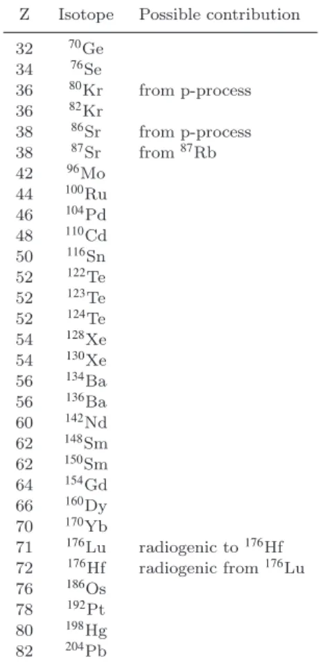
Table 1.List of 30 s-only isotopes adopted in this work
Z Isotope Possible contribution 32 70Ge 34 76Se 36 80Kr from p-process 36 82Kr 38 86Sr from p-process 38 87Sr from87Rb 42 96Mo 44 100Ru 46 104Pd 48 110Cd 50 116Sn 52 122Te 52 123Te 52 124Te 54 128Xe 54 130Xe 56 134Ba 56 136Ba 60 142Nd 62 148Sm 62 150Sm 64 154Gd 66 160Dy 70 170Yb 71 176Lu radiogenic to176Hf 72 176Hf radiogenic from176Lu 76 186Os 78 192Pt 80 198Hg 82 204Pb
may receive a non negligible contribution from the p-process (seeTravaglio et al. 2015). Moreover, there are isotopes with unstable isobars with (Z-1), whose lifetimes are compara-ble to the age of the Universe: in that case, therefore, a delayed r-process contribution cannot be excluded (e.g. for the couples87Sr-87Rb and187Os-187Re). Finally, there are a
few isotopes, with stable (Z-1) isobars, which may receive an important contribution from the neutrino process in core collapse supernovae (e.g.113In and115Sn; seeFujimoto et al.
2007). As a matter of fact, in the past different lists of s-only isotopes circulated in the literature. We list in Table1the s-only isotopes considered in this study, including those that may receive a small contribution from other processes (see
Travaglio et al. 2015).
The definition of r-only isotopes in even more ambigu-ous. In principle, at odds with s-only nuclei (shielded by the r-process from stable isobars), there is no nucleus fully shielded by the s-process. In fact, all nuclei on the neutron-rich side of the β-stability valley can receive a contribu-tion (perhaps very small, but not null) from the s-process, depending on the activation of various branchings. For in-stance, net yields from AGB stars byCristallo et al.(2015a) for isotopes marked as r-only in previous compilations (e.g.
Goriely 1999andSneden et al. 2008) are all positive (from some % to significant fractions, depending on the isotope), apart from130Te. In this study we shall not pre-define
”r-only” nuclei, but we shall explore with our method the con-tribution of our stellar yields to the abundances of all heavy isotopes.
3.2 Assumptions
The method adopted in this study is based on a couple of key assumptions.
Assumption 1: Our current understanding of stellar nucleosynthesis and galactic chemical evolution allows us to reproduce the pre-solar isotopic abundances to a precision of (a) a factor of ∼ 2 for elements with charge 2 < Z < 30 (between Li and Zn) but (b) to a factor of ∼20-30 % (or less) for the s-component of heavier elements.
Statement (a) above is based on the fact that all calcu-lations done up to now with ”state-of-the-art” stellar yields and models of the chemical evolution of the solar neighbor-hood show indeed a dispersion of a factor ∼2 around the solar value in the region up to the Fe-peak. This is true e.g. for the models ofTimmes et al.(1995), who adopted yields of Woosley & Weaver (1995), Goswami & Prantzos (2000) with yields of Woosley & Weaver (1995), Kubryk et al.
(2015) with yields ofNomoto et al.(2013) and Paper I with yields ofLimongi & Chieffi(2018). Even if in each case the adopted models and yields differ considerably, the outcome is the same: a dispersion by a factor of ∼2 is always found, implying that uncertainties in the various parameters of the problem (regarding both stellar and galactic physics) remain important in the past two decades or so.
Statement (b) is based on a limited sample of GCE mod-els, namely those of Travaglio et al.(2004), Cristallo et al.
(2015b) and Bisterzo et al. (2017) see previous section -as well -as our own model presented in Paper I. In those by
Travaglio et al.(2004) andBisterzo et al.(2017), the model values of most heavy pure s-nuclei barely exceeds the cor-responding solar value and there is a systematic deficiency of ∼20-30% as one moves to lighter s-nuclei. This deficiency was interpreted as evidence for the need of another heavy isotope component, the so-called LEPP (see previous sec-tion). However, Paper I showed that rotating massive stars may produce through the weak s-process that ”missing” com-ponent, with no need for a new process. In that study, it is found that most pure s-nuclei are co-produced within ∼10-20% from their pres-solar values, with only a few of them displaying higher values (up to 40% at most).
We think that it is illusory at the present stage of our knowledge to reproduce the pre-solar pure s-composition to a higher accuracy. We believe however that it is possible to use this result and try to infer the solar s- and r-components of all mixed (s+r) nuclei, as presented in Sec.3.3.
Assumption 2: The r-process is of ”primary” nature and, in particular, it mimics the behaviour of the ”alpha” process which produces α-elements like e.g. 16O. This
as-sumption is based on the observational fact that pure r-elements, like Eu, display an α-like behaviour, i.e. the ratio [Eu/Fe] remains ∼constant at a value of ∼0.3-0.5 dex dur-ing the late halo evolution and then declines smoothly to its solar value at [Fe/H]∼0. This means that, in contrast to the s-process, which is basically of ”secondary” nature (i.e. the s-yields of both LIM stars and massive stars depend on the abundance of iron-seed nuclei), the r-yields are indepen-dent of the initial metallicity of their source. The ratio of those yields to the yields of α-isotopes should then be con-stant with metallicity. These inferences allow one to adopt r-process yields ”scaled” to the stellar model yields used in the GCE model.
3.3 Method
Our ”bootstrap” method proceeds as follows:
Step 0: We run a GCE model as in Paper I but us-ing exclusively the s-component for all elements with Z>30. For that purpose we remove from the adopted yields the r-component (i.e. existing in the initial composition of the stars, through their scaled solar composition). In practice, we calculate a new set of yields as:
yi(M, Z) = yi,0(M, Z) − fr,i,0 Xi,⊙ Z Me j(M, Z) (1)
where:
• yi,0(M, Z)are the original yields of isotope i from stars of mass M and metallicity Z.
• fr,i,0 is the solar r-fraction of nucleus i, as provided i.e. inSneden et al.(2008) orGoriely(1999).
• Me j(M, Z)is the total mass ejected by the star of mass M and metallicity Z.
The results of the model at the time of Solar system for-mation (i.e. 4.56 Gyr before the end of the simulation) are stored as
Wi,0 = Xi,0/Xi,⊙ (2)
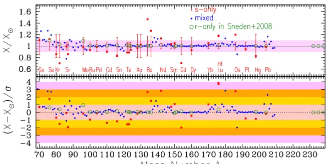
i.e., they are normalized to the corresponding Solar system isotopic abundances adopted from Lodders et al. (2009). These normalized abundances appear in the top panel of Fig.1for all nuclei with charge Z>30.
Among the s-only nuclei (red dots), most are reproduced within a factor of 20% solar abundances (see also Paper I5),
except Kr, Ba and Gd which differ from their solar values by 20-40 %.Taking into account the uncertainties in nuclear, stellar and galactic physics involved in the calculation, which lead to a larger dispersion for the lighter nuclei (up to 100 % , factor of ∼2, see Fig. 11 in Paper I), we think that this agreement is quite satisfactory.
In particular, regarding the nuclear uncertainties, we note that our results are obtained with nucleosynthesis cal-culations using the set of neutron capture cross sections de-scribed inStraniero et al.(2006). Since then, two new cross sections became available, i.e. those of176Lu (Wisshak et al.
2006a) and176Hf (Wisshak et al. 2006b). Both cross sections
are larger than those adopted to calculate our models, so that we expect a decrease for both isotopes (see Table1), thus providing a better agreement with observations. We ex-pect a similar behavior for134Ba (and possibly136Ba): both
neutron capture cross sections will be measured in the next years at the n TOF facility (Guerrero et al. 2013). More-over, we further stress that the abundance of134Ba strongly
depends on the activation of the branching at134Cs, whose
neutron capture cross section and temperature-dependent β-decay lifetime are rather uncertain. By varying theoreti-cal nuclear inputs within uncertainties in a single model, we can obtain a decrease of about 15% and 12% for134Ba and
5 Notice that with respect to Paper I we have slightly reduced here the proportion of fast rotating massive stars (at 300 kms−1) in our mixture, in order to avoid an overproduction of the lighter s-only nuclei like70Ge and76Se; this reduction affects correspond-ingly the results of80,82Kr (compare e.g. to Fig. 11 in Paper I) but no other nuclei, either lighter or heavier ones), since they are essentially produced by LIM stars.
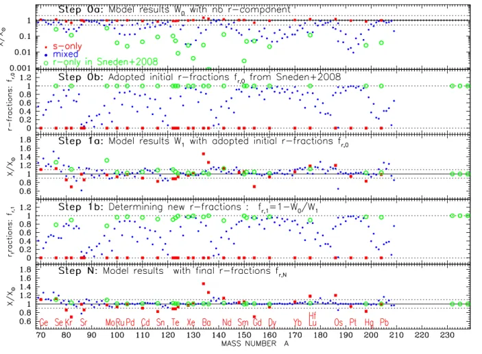
Figure 1. Top: Model results W0 after Step 0, without r-component (see text); horizontal dashed lines indicate levels of ±10% and a factor of 2 deviation from solar; 2ndfrom top: Adopted initial r-fractions fromSneden et al.(2008); 3rdfrom top: Results W
1after Step 1, with r-component introduced fromSneden et al.(2008) ; horizontal dashed lines indicate levels of ±10% deviation from solar; 4thfrom
top: Our r-component after Step 1 is obtained as r1= 1 − W0/W1 (where the corresponding s-component is obtained first as s1= W0/W1) and is introduced in the next iteration; Bottom: Same as the 3d panel, after the final (N=17 here) iteration of our ”bootstrap” method; horizontal dashed lines indicate levels of ±10% deviation from solar. Note that the scale in the Y-axis changes in the different panels.The names of the elements with s- only isotopes are indicated in the bottom panel.
136Ba, respectively (see alsoCristallo et al. 2015b; Goriely
1999). All the above concern s-only isotopes which are over-produced with respect to their pre-solar system values in Fig.1.
As for the s-only isotopes that are under-produced with respect to the solar distribution, we stress that the neu-tron capture cross section of 82Kr is quite uncertain at
typical s-process temperatures (∼25% at 8 keV; KADONIS database6). Moreover, it has to be stressed that the solar Kr
and Xe abundances are not directly measured in the Sun, but they ” are based on theoretical values from neutron-capture element systematics” (Lodders 2003). On the other hand, the synthesis of154Gd is strongly affected by the branching
at 154Eu. Its neutron capture cross section has never been
measured and its temperature-dependent β-decay lifetime is uncertain by a factor of three (Goriely 1999). Note that for
6 https://exp-astro.de/kadonis1.0/
the decay, no hints on its trend between 5×10⁷K and
labora-tory temperature is provided inTakahashi & Yokoi(1987). As already done for barium isotopes, if we just vary theo-retical nuclear inputs within uncertainties, we can obtain an increase of about 25% for154Gd7.
Finally, it should be emphasized that we did not make any attempt to adjust the parameters of the GCE model (distribution of stellar rotational velocities, initial mass func-tion or star formafunc-tion and infall rates) as to optimize the s-only distribution; as discussed in Paper I, our GCE model is tuned in order to reproduce as well as possible local pa-rameters like the current gas fraction, the metallicity distri-bution and age-metallicity relation and the abundances of major elements like O and Fe at Solar system formation.
7 Note that the154Gd neutron capture cross section has been re-cently measured at the n TOF facility (Massimi et al., in prepa-ration)
Despite that, we find that the parameter g = exp 1 nS nS X Z,A ln2Ncal(Z, A) N⊙(Z, A) 1/2 (3)
where the sum runs over the nS = 30 s-only nuclei (of charge Z and mass A, see Table 1) is g = 1.18, i.e. it is not much higher than the value of 1.10 obtained in Goriely (1999). This author optimized the few parameters of his multi-event model as to minimize g, while we did not attempt such an optimization here. (with a classical analysisGoriely (1999) found g = 1.44). Although our results are obtained with a dif-ferent method and data (nuclear cross sections, stellar condi-tions, solar abundances), we believe that our result regarding the s-only distribution is quite reasonable and constitutes a good starting point for our GCE method. We discuss a little more our distribution of the s-component of our GCE model in Sec. 4, where we present the resulting σANAdistribution.
We emphasize here that, in contrast to the GCE method ofTravaglio et al.(2004);Bisterzo et al.(2014,2017) we do not proceed directly after the first run to the evaluation of the solar s-component by subtracting our results from the solar composition. This might lead to the need of a LEPP to justify the underproduction of several s-only nuclei, as the aforementioned GCE studies did. We proceed in a different way, allowing us to keep the ”s-only” property of the isotopes of Table 1 and at the same time evaluate self-consistently the s-fraction of the mixed (s+r) isotopes. For that, we need to introduce a priori their r-fractions, as described below.
Step 1: We run a model by using now the original stellar yields yi,0(M, Z)and introducing this time the r-component
of each isotope as in Paper I, namely by assuming that it is co-produced with a typical product of massive stars like
16O, i.e. the new yield for massive stars (M>10 M ⊙) is
yi,1(M, Z) = yi,0(M, Z) + fr,i,0y16O(M, Z) Xi,⊙/X16O,⊙ (4)
where the last term represents the r- component of the yield and fr,i,0is an ”educated guess” for the solar r- fraction of
iso-tope i; we start by adopting the r- fractions ofSneden et al.
(2008) but our results are independent of that choise (see below).
The underlying physical assumption of Eq.4is that16O
and the r-component have the same source, namely massive stars and this implicit assumption allows one to reproduce naturally the observed alpha-like behaviour of elements that are mostly of r-origin, like e.g. Eu. The method can be used in essentially the same way in the case that the main source of r-process turns out to be a rare class of massive stars, like collapsars (see e.g.Siegel et al. 2019, and references therein). In that case a stochastic treatment should be made, e.g. as applied for neutron star mergers in Ojima et al. (2018). If neutron star mergers are assumed to be the site of the r-process, a different prescription should be used, involving the rate of occurrence of that site (through a delayed time distribution, as for SNIa, e.g.Cˆot´e et al. 2018) and the mass ejected in the form of isotope i, normalized as to get a solar abundance for the pure r-isotopes of Th and U.
Notice that in this run we treat all nuclei except the s-only ones of Table 1 as mixed s+r: those classified as pure r- inSneden et al.(2008) orGoriely(1999) are also treated as such. They are simply given an initial r-fraction fr,i,0=1,
which may change after Step 1.
The result of the new run is also plotted in Fig. 1for all isotopes with charge Z> 30 as overabundances
Wi,1 = Xi,1/Xi,⊙ (5)
where
Xi,1 = Xs,i,1 + Xr,i,1 (6)
with Xs,i,1= Xs,i,0(the s-component remains the same) and
Xr,i,1/Xi,⊙= C fr,i,0 (7)
is the r-component (proportional to the r-fraction fr,i)with
the constant C being the IMF average of the r-component term in Eq.4and adjusted as to obtain at Solar system for-mation the exact solar abundances of pure r-isotopes, like Th, which we use here as benchmarks8. The value of C
de-pends on the adopted ingredients of the GCE model (IMF, SF and infall rates, stellar yields) and it is ∼1.12 in our case.
One notices that:
• s-only isotopes are produced exactly at the same level as in step 0, since their yields have not been modified.
• r-only isotopes with the meaning discussed in §3.1are produced exactly at their pre-solar abundances -because of the adopted normalization in Eq.4and7- except a few of them which have received a non-zero contribution from the s-process in step 0 (see green symbols in top panel of Fig.
1) and are now slightly overproduced. The most prominent of them are76Ge (by ∼25%),82Se (∼10%),96Zr (∼30%) and 142Ce (∼15%), as shown in the 3rd panel of Fig.1.
• isotopes of mixed (s+r) origin are nicely co-produced w.r.t. their pre-solar abundances, to better than 10% in gen-eral, although in some regions (A∼ 205, 180, 138, < 95) they are overproduced by ∼20% and the overproduction reaches 40% for the lightest ones.
Obviously, by comparing the results of runs 0 and 1 (top and third from top panels) one may obtain the s-fraction of each mixed isotope as
fs,i,1 = Wi,0/Wi,1 = Wi,0/(Wi,0 + C fr,i,0) (8)
and the corresponding r-fraction as
fr,i,1 = 1 − fs,i,1 = 1 − Wi,0/(Wi,0 + C fr,i,0) (9)
This procedure was adopted in Paper I, albeit not for the pure r-isotopes for which we assumed a final r-fraction equal to the initial one fr=1. However, at this level the
method was obviously not self-consistent: the resulting r-residuals, obtained with Eq. 9were not the same as those used to run the model with the r-component in Eq.4. This is obvious in the 4th panel of Fig.1, in particular regarding
the r-fractions of76Ge (which is now ∼80% instead of 100%
initially) and82Se (now ∼90% instead of 100%).
Step 3: In this study, seeking for self-consistency, we proceed by injecting the obtained r-fractions of step 1 and Eq.9into the yields of Eq.4and running a new model. The results of the new model are identical with those of previous calculations regarding all isotopes below Z= 30 and the pure s-ones, but they fit slightly better the pre-solar distribution of mixed s+r isotopes.
8 The radioactive decay of Th and U isotopes is properly taken into account in our GCE model.
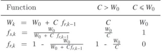
Table 2.Limits of recursive functions W, fs and frfor k → ∞ Function C > W0 C 6 W0 Wk = W0 + C fr,k−1 C W0 fs,k = W W0 0+ C fr,k−1 W0 C 1 fr,k = 1 - W0+ C fW0r,k−1 1 -W0 C 0
We evaluate the quality of the fit to the solar com-position through a simple χ2 test and we repeat running
the models injecting each time the new r-fraction obtained through Eq. 9 into the yields of mixed isotopes. The fit improves slower and slower as the number of iterations in-creases, until the improvement becomes negligible (less than 1 part in a thousand) and we stop. This happens in general after 10-20 iterations, depending on the initial r-fractions adopted9.
From the mathematical point of view, it can be easily shown that the quantities W (Eq.5), fs(Eq.8), and fr(Eq.
9), expressed as recursive functions, converge to the values indicated in Table2, depending on whether the constant C is greater or smaller than the initial overabundance W010, i.e.
the s- component. In other terms, our results for the s- and r- fractions depend uniquely on a) the adopted stellar yields of s-isotopes (which determine, along with the chemical evo-lution model, the term W0), and b) the goodness of the fit to
the pure r- isotopes of Th and U (which determine through Eq.4 and 7 the constant C), but they are independent of the choice of the initial values of fr,0.
The reason why this iterative method improves - albeit slightly - the overall fit is due to the fact that the sum of the s- and r- fractions for a mixed nucleus is always fs+ fr=1.
If the new s-fraction is found (Eq.8) to be smaller than the original one, then the new r-fraction is automatically found to be larger than the original one to compensate, and vice versa.
In the bottom panel of Fig. 1 we display the results of the final run. The agreement with pre-solar abundances is now considerably improved for the mixed (s+r) nuclei, which are reproduced to better than a few % in most cases. We consider this a satisfactory result and we believe that it is the best one may hope to get from current models of stellar nucleosynthesis and galactic chemical evolution.
We also repeated the procedure by adopting the initial r-residuals ofGoriely(1999) and we obtained quantitatively similar results for all mixed (s+r) isotopes, except for the few cases which are classified as pure s- or r- by Goriely
(1999) but not bySneden et al.(2008); these are cases where the minor residual has a very small contribution to the iso-topic abundance, typically less than a few %, which may be smaller than the uncertainties defined by the method of
Goriely(1999).
9 The number of iterations required to reach a given level of con-vergence increases with decreasing fr,0; for a level of 10
−2we find that 20-30 iterations are sufficient.
10 This can be trivially obtained by putting f
r= fr,0 in Eq.9
4 RESULTS AND DISCUSSION
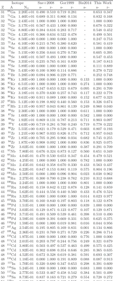
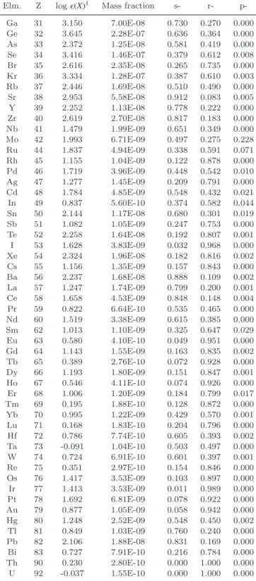
Our results concerning the s- and r- fractions of all the heavy isotopes are presented in Table 3, along with those ofGoriely(1999) andSneden et al. (2008) as well as those ofBisterzo et al.(2014); notice that for the latter we provide only the s-contribution (see below). For an easier compari-son with those studies, the data are also presented in Figs.2
and3. Although it is impossible (and rather meaningless) to perform a one-to-one comparison for each isotope, we notice some important features.
4.1 The s- and r- fractions
We start by displaying in Fig.2the results for heavy nuclei that have been classified as s-only (top) or r-only (bottom) in each of the studies ofGoriely(1999),Sneden et al.(2008) and the present one. We emphasize that in our study the nuclei considered as s-only in the beginning (Model 0) are also found to be s-only during the whole procedure and in the final model, since the adopted yields for those species are always the same (exactly as in the case of nuclei lighter than Z= 31). This does not mean that their final abundances match perfectly well the corresponding Solar system abun-dances. But we consider that the obtained deviations from the solar abundances are a natural feature of the adopted GCE method, reflecting the current limitations of 1-zone models of GCE (coming mainly from stellar yields).
Our method (dividing M0 by M1) allows us to attribute fs=1 to those nuclei that we pre-defined as s- only. This
is not the case with the other studies using GCE models (Travaglio et al. 2004;Bisterzo et al. 2014), which try to re-produce perfectly the solar abundances of s-only isotopes, something we think is illusory at present. This is why we postpone the discussion of our differences with those studies to Fig.3.
We notice that the s- and r-fractions displayed in Fig.
2 are evaluated in different ways for the three studies.
Sneden et al.(2008) provide the absolute numbers for both components s- and r- (Ns and Nr) for each heavy isotope,
in a scale where NSi≡106; in that case one has obviously:
fs=Ns/(Ns+Nr) and fr=Nr/(Ns+Nr).Goriely(1999) provides
only the Nr values, again in a scale NSi≡106, but he does not provide the corresponding Nsvalues; we obtain here the
corresponding Ns values by subtracting Nr from the total
isotopic abundances NT where we use the pre-solar ones of
Lodders et al.(2009), which were not available in 1999. This obviously introduces some systematic differences with the actual values found byGoriely(1999), hopefully small ones. We do not take into account a couple of nuclei considered as s-only in Goriely (1999), which we consider instead as p-nuclei, like152Gd and164Er.
Fig.2illustrates the difficulties to determine unambigu-ously whether an isotope is produced exclusively by one or the other of the two neutron capture processes. While
Goriely(1999) finds 36 s-only isotopes, we andSneden et al.
(2008) find only 30. For two of the six discrepant cases,94Zr
and 208Pb, we and Sneden et al. (2008) find quite high
s-fractions of more than 90%, i.e. almost pure s-nuclei. For two others (72Ge and 78Se) we both find a dominant
s-contribution of 55-65 %, which leaves room however, for a large r-contribution. Finally, there are two cases (86Kr
Figure 2. Top: Nuclei having an s-fraction fs=1 in at least one of the lists ofGoriely(1999),Sneden et al.(2008) or ours. Bottom: Nuclei with r-fraction fr= 1 in at least one of the cited studies. In parentheses: the number of such nuclei in each study. In the bottom panel: two numbers are given, for r- fractions fr>0.99and >0.97, respectively; the Th and U isotopes are counted in, even if they do not appear in the figure.
and 187Os) where Sneden et al. (2008) find a very high
s-contribution of more than 90% (making those nuclei almost s-only), while we find a smaller one, around 70-75%. It is hard to trace the exact origin of these differences, which can be broadly attributed to the different methods and data fol-lowed to derive the s- fractions. The abundance of 86Kr is
determined by the branching at85Kr; its activation largely
depends on the temperature and, as a consequence, requires the use of full stellar models to be properly treated. On the other hand, 187Os may receive an important contribution
from the decay of187Re during the long burning phases of
low and intermediate mass stars (the so-called ”astration” term of Yokoi et al. 1983). Unfortunately, such a decay is not known at temperatures intermediate between laboratory values and some tens of millions K, making the evaluation of the ”astration” term in full stellar evolutionary models very uncertain.
As for the r-only nuclei, the bottom panel of Fig. 2
shows that their number varies strongly with the adopted criterion for their definition. If an r-contribution fr>0.99 is
required, then only 8 nuclei fulfill it in our case, against 13 for
Goriely(1999) and 27 forSneden et al.(2008). If fr>0.97is
adopted instead, the corresponding numbers become 15, 18 and 32, respectively. Obviously, this reflects directly the diffi-culty to determine accurately the corresponding s-fractions, which are fairly small. The reason for the discrepancy be-tweenSneden et al.(2008) and the other two studies is quite probably the broader range of physical conditions (tempera-ture and neutron fluence) spanned in the multi-event study and this work, which allows the neutron flow to reach in some cases nuclei usually unreachable in the ”classical” method.
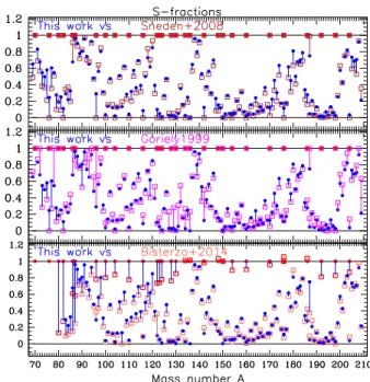
Figure 3.Our s-fractions (in blue in all panels) compared to results of three works obtained with different methods. Top:
Sneden et al.(2008) with the classical method. Middle: Goriely
(1999) with the multi-event method. Bottom: Bisterzo et al.
(2014) with a GCE model. Vertical lines connect same nuclei, their colour corresponding to the largest s-fraction of the two re-sults. Red circles indicate our s-only nuclei (see Table1).
The most characteristic cases are134,136Xe for whichGoriely
(1999) finds an r-contribution of ∼75% (against more than 97% in our case), and142Ce where he obtains 50% only while
we obtain 87% (see Table3).
The most significant discrepancy between those stud-ies is the case of96Zr. It is considered as a pure r-nucleus
inSneden et al.(2008), but we find only 70% whileGoriely
(1999) finds that its r-contribution is compatible with zero, i.e. that it may be a pure s-nucleus. The abundance of this nucleus strongly depends on the treatment of the branching at95Zr, which is activated during thermal pulses only (i.e.
when the temperature at the base of the convective shell exceeds 2.5 × 10⁸K). We notice that, in our models, the
con-tribution of the s-process (from LIM stars) is 30%, which is compatible with the 40 % s-contribution of Bisterzo et al.
(2014).
In Fig.3we present a more detailed comparison of our results to those ofSneden et al.(2008) (top panel),Goriely
(1999) (middle) andBisterzo et al.(2014) (bottom). We no-tice that there are few s-only nuclei (i.e. with fs∼1) in the
latter work, since they are not ”pre-defined”, as in our case. Thus, despite the use of a similar method to ours (GCE), the s-component of the heavy nuclei is identified in a different way inBisterzo et al. (2014) and this makes more difficult a direct comparison to our results. It turns out, however, that apart form the s-only nuclei, our results display largely similar features.
In the range A< 85, our results are systematically higher than Sneden et al. (2008) or Bisterzo et al. (2014) and rather closer toGoriely(1999). This is due to the fact that our adopted yields from rotating massive stars
(respon-Figure 4.Curve σANs,Aof the pre-solar system s-component, afterSneden et al.(2008) (brown open squares) and this work (all other
symbols). Our s-only nuclei appear as red crosses and are connected by a solid curve to guide the eye. The green open circles represent
nuclei that are r-only forSneden et al.(2008) (hence they should not appear on the figure), but they receive a small s- contribution in our work. Cross-sections are expressed in mb and number abundances Ns,A are in the meteoritic scale of NSi≡106.
sible for the weak s-process in that region of mass number) produce abundantly the light s-nuclei: as explained in Pa-per I, rotational mixing of 14N from the H-layer in the
He-core produces more 22Ne than in non-rotating models and
enhances substantially the neutron fluency and the result-ing s-isotope production (see alsoChoplin et al. 2016,2018). This leads to a larger s-process contribution to the isotopic abundances in that mass range.
The cases of 76Ge and82Se illustrate well theses
find-ings. They are classified as pure r-nuclei by Sneden et al.
(2008) and Goriely (1999) whereas our method leads to a 25% s-contribution to the former and a 11 % s-contribution to the latter, because of the rotating massive star yields.
In the region 85 <A< 200 our results are in fairly good quantitative agreement with Sneden et al. (2008), while
Goriely (1999) finds systematically higher s-fractions for 85 <A< 100 and 120 <A< 135. However, in all these cases the uncertainties in the determination of the s-fractions (as evaluated only byGoriely 1999) are substantial and the re-sults can be considered as compatible with each other. This is also true for several cases found to be pure r-isotopes by
Goriely(1999), while bothSneden et al.(2008) and us find a small s-contribution (e.g.153Eu,159Tb,161Dy).
In the region A> 200 Goriely (1999) has, in general, larger s-contributions than both Sneden et al. (2008) and us. His multi-event method results in a stronger ”strong” s-process component than the other studies.
Above A= 100 and up to the heaviest nuclei, our results are in excellent agreement with Bisterzo et al. (2014), ex-cept for the cases of the s-only nuclei (already discussed). This is the case of 142Ce which is a pure r-nucleus for
Sneden et al. (2008), while we find an s-contribution of ∼13% andBisterzo et al.(2014) find a 20% s-contribution. Finally, 187Os has a much larger s-contribution of 75% in
our case vs 37% inBisterzo et al.(2014), while it is a pure s-nucleus in bothSneden et al.(2008) andGoriely(1999).
4.2 The σANAcurve
The classical method to determinate the s-component of the heavy isotopes relies on the assumed constancy of the prod-uct σANs,A of the neutron capture cross section σA times
the number abundance Ns,Aof the s-component of the heavy
nuclei. In Fig.4we display that product for our results, ob-tained from our s-fraction from Table3, the corresponding Solar system isotopic abundance fromLodders et al.(2009) (also provided in Table 3) and the neutron capture cross sections at 30 keV provided in the KADONIS database11
(Dillmann et al. 2008).
Our σANs,A curve displays the ”classical” features,
namely, a decrease up to A∼90, a near constant value up to the 2ndpeak at A∼135 (the Ba isotopes), then a small
de-cline and again an approximately constant value up to the 3rd peak at A∼205 (the Pb isotopes). We notice, however,
that the σANs,Aproduct of s-only nuclei (red cross symbols,
connected with a solid curve) is not constant in the whole range of A before the 3rd peak, but it declines by almost a
factor of 2 between A= 160 and A= 190; this would make it difficult to derive accurately with the classical method the s-only abundances of isotopes in that mass range, at least with the sets of σA and Ns,A adopted here.
In Fig.4we also present the σANs,A product obtained
with the s-component ofSneden et al.(2008), multiplied by the same set of cross-sections as in our case. In that way, the differences between the two sets of results depend only on the s-residuals, which are obtained by two different meth-ods. Although the s-residuals of Sneden et al. (2008) were obtained by using the σANA method with a different set of
cross-sections (older than the one used here and presumably less accurate), still it is interesting to compare the two sets of results.
There is fairly good agreement for a large range of mass
Figure 5.Results compared to uncertainties of pre-solar abundances. Top: Model over-abundances at the time of Solar system formation and elementary uncertainties ±1σ for the s- only isotopes (vertical red segments, centered at X/X⊙=1 fromLodders et al.(2009), the names of which are provided in the bottom of the panel; the shaded area indicates the range of ±10% deviation from solar. Bottom: Overabundances (positive) or underabundances (negative) expressed in terms of the corresponding elementary uncertainties. Shadowed areas indicate ranges of ±1σ, ±2σ, etc.
numbers (90 < A < 190). There are, however, important dis-crepancies (by factor of ∼2) in the range of light s-nuclei, for 74 <A< 87; this is not surprising, since σANs,Ais not expected
to be constant in that atomic mass region, making it difficult to derive the s-component with the classical method.
The most important differences between the two results concern:
• The three nuclei76Ge,82Se and96Zr, which are pure r-nuclei (open circles in the figure) in both Goriely (1999) and Sneden et al. (2008) but are found to receive an s-contribution of 25%, 11% and 30%, respectively, from our s-process, the first two from rotating massive stars and the third from LIM stars.
• Several other nuclei, which are considered pure r-nuclei in Sneden et al.(2008) but have s-contribution in our case and inGoriely(1999). In most cases that contribution is of a few %, but it mounts to 10% for116Cd,142Ce and176Yb;
similar results for the s-contribution of all those nuclei are obtained inBisterzo et al.(2014).
• Nuclei lying near branching points, like 148Nd, 170Er and 192Os, which receive a fairly small s-contribution in
Sneden et al. (2008) but a considerably larger one (factors 2-4 larger) in our case
We notice that in the last two cases, our results agree fairly well with those of Goriely (1999) and Bisterzo et al.
(2014), probably because these studies explore more realis-tic physical conditions in stellar interiors than the classical study ofSneden et al. (2008) could do. We consider this is an important advantage of those methods over the classi-cal one in determining the s-fractions - and, thereoff, the r-fractions - of the solar composition.
4.3 Comparison to Solar system abundances
In the previous sub-sections we presented our s- and r-fractions of the heavy isotopes and we compared them to those of previous studies, pointing out similarities and dis-crepancies. In some cases we were able to attribute those discrepancies in differences in the adopted data and meth-ods. We also presented our σANs,A curve, which constitutes
an important criterion of the validity of our method; we showed that it succeeds fairly well and in some cases (e.g. the nuclei in branching points) even better than the classical method.
In this sub-section we present the abundances of all heavy isotopes (already displayed in the bottom panel of Fig.1) and we compare them to the Solar system ones, tak-ing into account the measurement uncertainties of the latter. As we emphasized in Paper I, our results strongly depend on the adopted yields of LIM stars and rotating massive stars, but also on the adopted chemical evolution model, because of the extreme sensitivity of the s-process yields to stellar metallicity. We also reiterate here two of our main findings in Paper I, namely that a) rotating massive stars contribute the bulk of the weak s-process up to A∼90 (and very little above it) while low mass stars are major s-contributors for A>90, and b) we find no compelling evidence for the LEPP invoked inTravaglio et al.(2004), especially if uncertainties in measured Solar system abundances are taken into account (see Fig. 11 and Sec. 3.2.2 of that paper).
In the top panel of Fig.5it is seen that the vast majority of the heavy isotopes (120 out of a list of 149, from which the p-isotopes are excluded) lie within ±10% of their solar values, while 96 of them lie within ±5%. However, among the