Symmetry for extremal functions in subcritical
Caffarelli-Kohn-Nirenberg inequalities
Jean Dolbeault
a, Maria J. Esteban
a, Michael Loss
b, and Matteo Muratori
caCeremade, UMR CNRS n◦7534, Université Paris-Dauphine, PSL research university, Place de Lattre de Tassigny, 75775 Paris 16, France bSchool of Mathematics, Georgia Institute of Technology, Skiles Building, Atlanta GA 30332-0160, USA
cDipartimento di Matematica Felice Casorati, Università degli Studi di Pavia, Via A. Ferrata 5, 27100 Pavia, Italy
Abstract
We use the formalism of the Rényi entropies to establish the symmetry range of extremal functions in a family of subcriti-cal Caffarelli-Kohn-Nirenberg inequalities. By extremal functions we mean functions which realize the equality case in the inequalities, written with optimal constants. The method extends recent results on critical Caffarelli-Kohn-Nirenberg in-equalities. Using heuristics given by a nonlinear diffusion equation, we give a variational proof of a symmetry result, by establishing a rigidity theorem: in the symmetry region, all positive critical points have radial symmetry and are therefore equal to the unique positive, radial critical point, up to scalings and multiplications. This result is sharp. The condition on the parameters is indeed complementary of the condition which determines the region in which symmetry breaking holds as a consequence of the linear instability of radial optimal functions. Compared to the critical case, the subcritical range requires new tools. The Fisher information has to be replaced by Rényi entropy powers, and since some invariances are lost, the estimates based on the Emden-Fowler transformation have to be modified.
Symmétrie des fonctions extrémales pour des inégalités de Caffarelli-Kohn-Nirenberg sous-critiques
Nous utilisons le formalisme des entropies de Rényi pour établir le domaine de symétrie des fonctions extrémales dans une famille d’inégalités de Caffarelli-Kohn-Nirenberg sous-critiques. Par fonctions extrémales, il faut comprendre des fonctions qui réalisent le cas d’égalité dans les inégalités écrites avec des constantes optimales. La méthode étend des résultats récents sur les inégalités de Caffarelli-Kohn-Nirenberg critiques. En utilisant une heuristique donnée par une équation de diffusion non-linéaire, nous donnons une preuve variationnelle d’un résultat de symétrie, grâce à un théorème de rigidité : dans la région de symétrie, tous les points critiques positifs sont à symétrie radiale et sont par conséquent égaux à l’unique point critique radial, positif, à une multiplication par une constante et à un changement d’échelle près. Ce résultat est optimal. La condition sur les paramètres est en effet complémentaire de celle qui définit la région dans laquelle il y a brisure de symétrie du fait de l’instabilité linéaire des fonctions radiales optimales. Comparé au cas critique, le domaine sous-critique nécessite de nouveaux outils. L’information de Fisher doit être remplacée par l’entropie de Rényi, et comme certaines invariances sont perdues, les estimations basées sur la transformation d’Emden-Fowler doivent être modifiées.
Keywords : Functional inequalities ; interpolation ; Caffarelli-Kohn-Nirenberg inequalities ; weights ; optimal functions ; best
constants ; symmetry ; symmetry breaking ; semilinear elliptic equations ; rigidity results ; uniqueness ; flows ; fast diffusion equation ; carré du champ ; Emden-Fowler transformation
Mathematics Subject Classification (2010) : Primary : 26D10 ; 35B06 ; 35J20. Secondary : 49K30 ; 35J60 ; 35K55.
Email addresses:[email protected](Jean Dolbeault),[email protected](Maria J. Esteban), [email protected](Michael Loss),[email protected](Matteo Muratori).
1. A family of subcritical Caffarelli-Kohn-Nirenberg interpolation inequalities With the norms
kwkLq,γ(Rd):= µZ Rd|w| q |x|−γd x ¶1/q , kwkLq(Rd):= kwkLq,0(Rd), let us define Lq,γ(Rd) as the space of all measurable functions w such that kwk
Lq,γ(Rd)is finite. Our functional framework is a space Hpβ,γ(Rd) of functions w ∈ Lp+1,γ(Rd) such that ∇w ∈ L2,β(Rd), which is defined as the completion of the space D(Rd\{0}) of the smooth functions on Rdwith compact support in Rd\{0}, with respect to the norm given by kwk2:= (p
⋆− p) kwk2Lp+1,γ(Rd)+ k∇wk2L2,β(Rd).
Now consider the family of Caffarelli-Kohn-Nirenberg interpolation inequalities given by kwkL2p,γ(Rd)≤Cβ,γ,pk∇wkϑL2,β(Rd)kwk1−ϑLp+1,γ(Rd) ∀ w ∈ H
p β,γ(R
d). (1)
Here the parameters β, γ and p are subject to the restrictions d ≥ 2, γ − 2 < β <d − 2
d γ , γ ∈ (−∞,d), p ∈ ¡
1, p⋆¤ with p⋆:= d − γ
d − β − 2 (2)
and the exponent ϑ is determined by the scaling invariance, i.e.,
ϑ = (d − γ)(p − 1)
p¡d + β + 2 − 2γ − p (d − β − 2)¢ .
These inequalities have been introduced, among others, by L. Caffarelli, R. Kohn and L. Nirenberg in [5]. We observe that ϑ = 1 if p = p⋆, a case which has been dealt with in [14], and we shall focus on the sub-critical
case p < p⋆. Throughout this paper,Cβ,γ,p denotes the optimal constant in (1). We shall say that a function w ∈ Hpβ,γ(R
d) is an extremal function for (1) if equality holds in the inequality.
Symmetry in (1) means that the equality case is achieved by Aubin-Talenti type functions w⋆(x) =
³
1 + |x|2+β−γ´−1/(p−1) ∀ x ∈ Rd.
On the contrary, there is symmetry breaking if this is not the case, because the equality case is then achieved by a non-radial extremal function. It has been proved in [4] that symmetry breaking holds in (1) if
γ < 0 and βFS(γ) < β <d − 2 d γ (3) where βFS(γ) := d − 2 − q (γ − d)2− 4(d − 1).
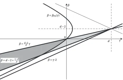
For completeness, we will give a short proof of this result in Section 2. Our main result shows that, under Condi-tion (2), symmetry holds in the complement of the set defined by (3), which means that (3) is the sharp condiCondi-tion for symmetry breaking. See Fig. 1.
Theorem 1.1 Assume that (2) holds and that
β ≤ βFS(γ) if γ < 0. (4)
Then the extremal functions for (1) are radially symmetric and, up to a scaling and a multiplication by a con-stant, equal to w⋆.
The result is slightly stronger than just characterizing the range of (β,γ) for which equality in (1) is achieved by radial functions. Actually our method of proof allows us to analyze the symmetry properties not only of
Figure 1. In dimension d = 4, with p = 1.2, the grey area corresponds to the cone determined by d − 2 + (γ − d)/p ≤ β < (d − 2)γ/d and
γ ∈ (−∞,d) in (2). The light grey area is the region of symmetry, while the dark grey area is the region of symmetry breaking. The threshold is determined by the hyperbola (d − γ)2− (β − d + 2)2− 4(d − 1) = 0 or, equivalently β = βFS(γ). Notice that the condition p ≤ p⋆induces the restrictionβ ≥ d − 2 + (γ − d)/p, so that the region of symmetry is bounded. The largest possible cone is achieved as p → 1 and is limited from below by the conditionβ > γ − 2.
extremal functions of (1), but also of all positive solutions in Hpβ,γ(Rd) of the corresponding Euler-Lagrange equations, that is, up to a multiplication by a constant and a dilation, of
−div¡|x|−β∇w¢= |x|−γ¡w2p−1− wp¢ in Rd\ {0}. (5)
Theorem 1.2 Assume that (2) and (4) hold. Then all positive solutions to (5) in Hpβ,γ(Rd) are radially symmetric and, up to a scaling and a multiplication by a constant, equal to w⋆.
Up to a multiplication by a constant, we know that all non-trivial extremal functions for (1) are non-negative solutions to (5). Non-negative solutions to (5) are actually positive by the standard Strong Maximum principle. Theorem 1.1 is therefore a consequence of Theorem 1.2. In the particular case when β = 0, the condition (2) amounts to d ≥ 2, γ ∈ (0,2), p ∈¡1,(d − γ)/(d − 2)¤, and (1) can be written as
kwkL2p,γ(Rd)≤C0,γ,pk∇wkϑL2(Rd)kwk1−ϑLp+1,γ(Rd) ∀ w ∈ H p
0,γ(Rd).
In this case, we deduce from Theorem 1.1 that symmetry always holds. This is consistent with a previous re-sult (β = 0 and γ > 0, close to 0) obtained in [17]. A few other cases were already known. The Caffarelli-Kohn-Nirenberg inequalities that were discussed in [14] correspond to the critical case θ = 1, p = p⋆or, equivalently β = d − 2 + (γ − d)/p. Here by critical we simply mean that kwkL2p,γ(Rd)scales like k∇wkL2,β(Rd). The limit case β = γ − 2 and p = 1, which is an endpoint for (2), corresponds to Hardy-type inequalities: there is no extremal function, but optimality is achieved among radial functions: see [16]. The other endpoint is β = (d − 2)γ/d, in which case p⋆= d/(d − 2). The results of Theorem 1.1 also hold in that case with p = p⋆= d/(d − 2), up to
existence issues: according to [9], either γ ≥ 0, symmetry holds and there exists a symmetric extremal function, or γ < 0, and then symmetry is broken but there is no optimal function.
Inequality (1) can be rewritten as an interpolation inequality with same weights on both sides using a change of variables. Here we follow the computations in [4] (also see [14,15]). Written in spherical coordinates for a function
e
w(r,ω) = w(x), with r = |x| and ω = x |x|,
inequality (1) becomes µZ∞ 0 Z Sd −1| ew| 2prd −γ−1d r dω¶ 1 2p ≤Cβ,γ,p µZ∞ 0 Z Sd −1|∇ ew| 2rd −β−1d r dω¶ ϑ 2µZ∞ 0 Z Sd −1| ew| p+1rd −γ−1d r dω¶ 1−ϑ p+1 where |∇ ew|2=¯¯∂ e∂rw ¯ ¯2+ 1 r2 |∇ωw|e 2and ∇
ωw denotes the gradient of ee w with respect to the angular variableω ∈ Sd −1. Next we consider the change of variables r 7→ s = rα,
e
w(r,ω) = v(s,ω) ∀(r,ω) ∈ R+× Sd −1 (6)
where α and n are two parameters such that
n =d − β − 2
α + 2 =
d − γ α . Our inequality can therefore be rewritten as
µZ∞ 0 Z Sd −1|v| 2psn−1d s dω¶ 1 2p ≤Kα,n,p µZ∞ 0 Z Sd −1 ³ α2¯¯∂v∂s¯¯2+s12|∇ωv|2 ´ sn−1d s dω ¶ϑ 2µZ∞ 0 Z Sd −1|v| p+1sn−1d s dω¶ 1−ϑ p+1 , with Cβ,γ,p= αζKα,n,p and ζ :=ϑ 2+ 1 − ϑ p + 1− 1 2 p= (β + 2 − γ)(p − 1) 2 p¡d + β + 2 − 2γ − p (d − β − 2)¢ . Using the notation
Dαv = µ α∂v ∂s, 1 s∇ωv ¶ , with α = 1 +β − γ 2 and n = 2 d − γ β + 2 − γ,
Inequality (1) is equivalent to a Gagliardo-Nirenberg type inequality corresponding to an artificial dimension n or, to be precise, to a Caffarelli-Kohn-Nirenberg inequality with weight |x|n−din all terms. Notice that
p⋆= n n − 2. Corollary 1.3 Assume thatα, n and p are such that
d ≥ 2, α > 0, n > d and p ∈¡1, p⋆¤.
Then the inequality
kvkL2p,d−n(Rd)≤Kα,n,pkDαvkϑL2,d−n(Rd)kvk1−ϑLp+1,d−n(Rd) ∀ v ∈ H
p
d −n,d−n(R
d), (7)
holds with optimal constantKα,n,p= α−ζCβ,γ,p as above and optimality is achieved among radial functions if
and only if
α ≤ αFS with αFS:=
s d − 1
n − 1. (8)
When symmetry holds, optimal functions are equal, up to a scaling and a multiplication by a constant, to v⋆(x) :=¡1 + |x|2¢−1/(p−1) ∀ x ∈ Rd.
We may notice that neither αFSnor βFSdepend on p and that the curve α = αFSdetermines the same
V. Felli and M. Schneider, who proved in [19] the linear instability of all radial critical points if α > αFS. When p = p⋆, symmetry holds under Condition (8) as was proved in [14]. Our goal is to extend this last result to the
subcritical regime p ∈ (1,p⋆).
The change of variables s = rαis an important intermediate step, because it allows to recast the problem as a more standard interpolation inequality in which the dimension n is, however, not necessarily an integer. Actually n plays the role of a dimension in view of the scaling properties of the inequalities and, with respect to this dimension, they are critical if p = p⋆and sub-critical otherwise. The critical case p = p⋆has been studied
in [14] using tools of entropy methods, a critical fast diffusion flow and, in particular, a reformulation in terms of a generalized Fisher information. In the subcritical range, we shall replace the entropy by a Rényi entropy power as in [21,18], and make use of the corresponding fast diffusion flow. As in [14], the flow is used only at heuristic level in order to produce a well-adapted test function. The core of the method is based on the Bakry-Emery computation, also known as the carré du champ method, which is well adapted to optimal interpolation inequalities: see for instance [2] for a general exposition of the method and [12,13] for its use in presence of nonlinear flows. Also see [6] for earlier considerations on the Bakry-Emery method applied to nonlinear flows and related functional inequalities in unbounded domains. However, in non-compact manifolds and in pres-ence of weights, integrations by parts have to be justified. In the critical case, one can rely on an additional invariance to use an Emden-Fowler transformation and rewrite the problem as an autonomous equation on a cylinder, which simplifies the estimates a lot. In the subcritical regime, estimates have to be adapted since after the Emden-Fowler transformation, the problem in the cylinder is no longer autonomous.
This paper is organized as follows. We recall the computations which characterize the linear instability of radially symmetric minimizers in Section 2. In Section 3, we expose the strategy for proving symmetry in the subcritical regime when there are no weights. Section 4 is devoted to the Bakry-Emery computation applied to Rényi entropy powers, in presence of weights. This provides a proof of our main results, if we admit that no boundary term appears in the integrations by parts in Section 4. To prove this last result, regularity and decay estimates of positive solutions to (5) are established in Section 5, which indeed show that no boundary term has to be taken into account (see Proposition 5.1).
2. Symmetry breaking
For completeness, we summarize known results on symmetry breaking for (1). Details can be found in [4]. With the notations of Corollary 1.3, let us define the functional
J [v] := ϑ log¡kDαvk L2,d−n(Rd) ¢ + (1 − ϑ) log¡kvkLp+1,d−n(Rd) ¢ + logKα,n,p− log¡kvk L2p,d−n(Rd) ¢
obtained by taking the difference of the logarithm of the two terms in (7). Let us define dµδ:= µδ(x)d x, where µδ(x) := 1
(1 + |x|2)δ.
Since v⋆as defined in Corollary 1.3 is a critical point of J , a Taylor expansion at order ε2shows that
kDαv⋆k2 L2,d−n(Rd)J £ v⋆+ εµδ/2f¤=12ε2ϑ Q[ f ] + o(ε2) with δ =p−12 p and Q[ f ] = Z Rd| Dαf |2|x|n−ddµδ−4 p α 2 p − 1 Z Rd|f | 2 |x|n−ddµδ+1. The following Hardy-Poincaré inequality has been established in [4].
Z Rd| Dαf |2|x|n−ddµδ≥ Λ Z Rd|f | 2 |x|n−ddµδ+1 (9)
holds for any f ∈ L2(Rd,|x|n−ddµδ+1), withDαf ∈ L2(Rd,|x|n−ddµδ), such thatR
Rdf |x|n−ddµδ+1= 0, with an optimal constant Λ given by
Λ= 2α2(2δ − n) if 0 < α2≤ (d − 1)δ 2 n (2δ − n)(δ − 1), 2α2δ η if α2> (d − 1)δ 2 n (2δ − n)(δ − 1), whereη is the unique positive solution to
η (η + n − 2) =d − 1 α2 .
Moreover, Λ is achieved by a non-trivial eigenfunction corresponding to the equality in (9). If α2>n (2(d−1)δδ−n)(δ−1)2 , the eigenspace is generated byϕi(s,ω) = sηωi, with i = 1, 2,. . . d and the eigenfunctions are not radially sym-metric, while in the other case the eigenspace is generated by the radially symmetric eigenfunctionϕ0(s,ω) = s2−2δ−nn .
As a consequence, Q is a nonnegative quadratic form if and only if 4 p αp−12 ≤ Λ. Otherwise, Q takes negative values, and a careful analysis shows that symmetry breaking occurs in (1) if
2α2δ η <4 p α 2 p − 1 ⇐⇒ η < 1, which means d − 1 α2 = η(η + n − 2) < n − 1, and this is equivalent to α > αFS.
3. The strategy for proving symmetry without weights
Before going into the details of the proof we explain the strategy for the case of the Gagliardo-Nirenberg inequalities without weights. There are several ways to compute the optimizers, and the relevant papers are [11,7,8,6,2,18] (also see additional references therein). The inequality is of the form
kwkL2p(Rd)≤C0,0,pk∇wkϑL2(Rd)kwk1−ϑLp+1(Rd) with 1 < p < d d − 2 (10) and ϑ = d (p − 1) p¡d + 2 − p (d − 2)¢ .
It is known through the work in [11] that the optimizers of this inequality are, up to multiplications by a constant, scalings and translations, given by
w⋆(x) =¡1 + |x|2¢−
1
p−1 ∀ x ∈ Rd.
In our perspective, the idea is to use a version of the carré du champ or Bakry-Emery method introduced in [1]: by differentiating a relevant quantity along the flow, we recover the inequality in a form which turns out to be sharp. The version of the carré du champ we shall use is based on the Rényi entropy powers whose concavity as a function of t has been studied by M. Costa in [10] in the case of linear diffusions (see [21] and references
therein for more recent papers). In [23], C. Villani observed that the carré du champ method gives a proof of the logarithmic Sobolev inequality in the Blachman-Stam form, also known as the Weissler form: see [3,24]. G. Savaré and G. Toscani observed in [21] that the concavity also holds in the nonlinear case, which has been used in [18] to give an alternative proof of the Gagliardo-Nirenberg inequalities, that we are now going to sketch.
The first step consists in reformulating the inequality in new variables. We set u = w2p,
which is equivalent to w = um−1/2, and consider the flow given by ∂u ∂t = ∆u m, (11) where m is related to p by p = 1 2m − 1. The inequalities 1 < p < d d −2imply that 1 −1 d< m < 1. (12)
For some positive constant κ > 0, one easily finds that the so-called Barenblatt-Pattle functions u⋆(t, x) = κdt− d d m−d+2w2p ⋆ ³ κ t−d m−d+21 x ´ =¡a + b |x|2¢− 1 1−m
are self-similar solutions of (11), where a = a(t) and b = b(t) are explicit. Thus, we see that w⋆= u⋆m−1/2is
an optimizer for (10) for all t and it makes sense to rewrite (10) in terms of the function u. Straightforward computations show that (10) can be brought into the form
µZ
Rdu d x
¶(σ+1)m−1
≤ C Eσ−1I where σ = 2
d (1 − m)− 1 (13)
for some constant C which does not depend on u, where E :=
Z
Rdu m
d x
is a generalized Ralston-Newman entropy, also known in the literature as Tsallis entropy, and I :=
Z
Rdu |∇
P|2d x
is the corresponding generalized Fisher information. Here we have introduced the pressure variable
P= m
1 − mum−1. The Rényi entropy power is defined by
F := Eσ
as in [21,18]. With the above choice of σ, F is an affine function of t if u = u⋆. For an arbitrary solution of (11),
we aim at proving that it is a concave function of t and that it is affine if and only if u = u⋆. For further
refer-ences on related issues see [11,22]. Note that one of the motivations for choosing the variablePis that it has a
particular simple form for the self-similar solutions, namely
P⋆= m
1 − m ¡
a + b |x|2¢. Differentiating E along the flow (11) yields
so that
F′= σ(1 − m)G with G := Eσ−1I . More complicated is the derivative for the Fisher information:
I′= −2 Z Rdu mhTr³¡HessP −1d∆PId ¢2´ +¡m − 1 +d1 ¢ (∆P)2id x .
Here HessPand Id are respectively the Hessian ofPand the (d × d) identity matrix. The computation can be
found in [18]. Next we compute the second derivative of the Rényi entropy power F with respect to t: (F )′′ σ Eσ = (σ − 1) E′2 E2+ E′′ E = (σ − 1)(1 − m) 2I2 E2+ (1 − m) I′ E =: (1 − m)H . With σ =d2 1 1−m− 1, we obtain H = −2DTr³¡HessP−1 d∆PId ¢2´E + (1 − m)(1 − σ)(∆P− 〈∆P〉)2® (14)
where we have used the notation
〈A〉 := R RdumA d x R Rdumd x . Note that by (12), we have that σ > 1 and hence we find that F′′= (Eσ)′′
≤ 0, which also means that G = Eσ−1I is a non-increasing function. In fact it is strictly decreasing unlessPis a polynomial function of order two in x
and it is easy to see that the expression (14) vanishes precisely whenPis of the form a + b |x − x0|2, where a,
b ∈ R, x0∈ Rdare constants (but a and b may still depend on t).
Thus, while the left side of (13) stays constant along the flow, the right side decreases. In [18] it was shown that the right side decreases towards the value given by the self-similar solutions u⋆and hence proves (10) in
the sharp form. In our work we pursue a different tactic. The variational equation for the optimizers of (10) is given by
−∆w = a w2 p−1− b wp. A straightforward computation shows that this can be written in the form
2m um−2div¡u ∇P¢+ |∇P|2+ c1um−1= c2
for some constants c1, c2whose precise values are explicit. This equation can also be interpreted as the
varia-tional equation for the sharp constant in (13). Hence, multiplying the above equation by ∆umand integrating
yields Z Rd £ 2m um−2div¡u ∇P¢+ |∇P|2¤ ∆umd x + c1 Z Rdu m−1∆um d x = c2 Z Rd∆u m d x = 0.
We recover the fact that, in the flow picture, H is, up to a positive factor, the derivative of G and hence vanishes. From the observations made above we conclude thatPmust be a polynomial function of order two in x. In
this fashion one obtains more than just the optimizers, namely a classification of all positive solutions of the variational equation. The main technical problem with this method is the justification of the integrations by parts, which in the case at hand, without any weight, does not offer great difficulties: see for instance [6]. This strategy can also be used to treat the problem with weights, which will be explained next. Dealing with weights, however, requires some special care as we shall see.
4. The Bakry-Emery computation and Rényi entropy powers in the weighted case
Let us adapt the above strategy to the case where there are weights in all integrals entering into the inequality, that is, let us deal with inequality (7) instead of inequality (10). In order to define a new, well-adapted fast
diffusion flow, we introduce the diffusion operator Lα= −D∗αDα, which is given in spherical coordinates by Lαu = α2 µ u′′+n − 1 s u ′¶+ 1 s2∆ωu
where ∆ωdenotes the Laplace-Betrami operator acting on the (d − 1)-dimensional sphere Sd −1of the angular variables, and′denotes here the derivative with respect to s. Consider the fast diffusion equation
∂u ∂t = Lαu
m (15)
in the subcritical range 1 −n1< m = 1 −
1
ν< 1. The exponents m in (15) and p in (7) are related as in Section 3 by
p = 1 2m − 1 ⇐⇒ m = p + 1 2 p and ν is defined by ν := 1 1 − m. We consider the Fisher information defined as
I [P] :=
Z
Rdu |
DαP|2dµ with P= m
1 − mum−1 and dµ = sn−1d s dω = sn−dd x .
HerePis the pressure variable. Our goal is to prove thatPtakes the form a + b s2, as in Section 3. It is useful to
observe that (15) can be rewritten as
∂u ∂t =D
∗
α(uDαP) and, in order to computed I
dt , we will also use the fact thatPsolves ∂P
∂t = (1 − m)PLαP− |DαP|
2. (16)
4.1. First step: computation ofdI dt Let us define K [P] := A [P] − (1 − m)(LαP)2 where A [P] :=1 2Lα|DαP| 2−D αP·DαLαP and, on the boundary of the centered ball Bsof radius s, the boundary term
b(s) := Z ∂Bs ³ ∂ ∂s ³ Pm−1m |DαP|2´− 2(1 − m)Pm−1m P′LαP´dς = sn−1 µZ Sd −1 ³ ∂ ∂s ³ Pm−1m |DαP|2´− 2(1 − m)Pm−1m P′LαP´dω ¶ (s), (17) where by dς = sn−1dω we denote the standard Hausdorff measure on ∂Bs.
Lemma 4.1 If u solves (15) and if
lim s→0+ b(s) = lim S→+∞ b(S) = 0, (18) then, d dtI [P] = −2 Z RdK [ P]umdµ . (19)
Using (15) and (16), we can compute d dt Z A(s,S)u | DαP|2dµ = Z A(s,S) ∂u ∂t |DαP| 2d µ + 2 Z A(s,S) uDαP·Dα∂P ∂t dµ = Z A(s,S) Lα(um)|DαP|2dµ + 2 Z A(s,S) uDαP·Dα³(1 − m)PLαP− |DαP|2´dµ = Z A(s,S) umLα|DαP|2dµ + 2(1 − m) Z A(s,S) uP DαP·DαLαPdµ +2(1 − m) Z A(s,S) uDαP·DαPLαPdµ − 2 Z A(s,S) uDαP·Dα|DαP|2dµ +α2 Z ∂BS ³ (um)′|DαP|2− um ∂ ∂s(|DαP| 2)´dς −α2 Z ∂Bs ³ (um)′|DαP|2− um ∂ ∂s(|DαP| 2)´dς = − Z A(s,S) umLα|DαP|2dµ + 2(1 − m) Z A(s,S) uP DαP·DαLαPdµ +2(1 − m) Z A(s,S) uDαP·DαPLαPdµ +α2 Z ∂BS ³ (um)′|DαP|2+ um ∂ ∂s(|DαP| 2)´dς −α2 Z ∂Bs ³ (um)′ |DαP|2+ um ∂ ∂s(|DαP| 2)´dς ,
where the last line is given by an integration by parts, upon exploiting the identity uDαP= −Dα(um):
Z A(s,S) uDαP·Dα|DαP|2dµ = − Z A(s,S) Dα(um) ·Dα|DαP|2dµ = Z A(s,S) umLα|DαP|2dµ − α2 Z ∂BS um ∂∂s(|DαP|2)d ς + α2 Z ∂Bs um ∂∂s(|DαP|2)d ς.
1) Using the definition of A [P], we get that
− Z A(s,S) umLα|DαP|2dµ = −2 Z A(s,S) umA [P]dµ − 2 Z A(s,S) umDαP·DαLαPdµ . (20)
2) Taking advantage again of uDαP= −Dα(um), an integration by parts gives Z A(s,S) uDαP·DαPLαPdµ = − Z A(s,S) Dα(um) ·DαPLαPdµ = Z A(s,S) um(LαP)2dµ + Z A(s,S) umDαP·DαLαPdµ − α2 Z ∂BS umP′LαPdς + α2 Z ∂Bs umP′LαPdς . and, with uP= m 1−mum, we find that
2(1 − m) Z A(s,S) uP DαP·DαLαPdµ + 2(1 − m) Z A(s,S) uDαP·DαPLαPdµ = 2(1 − m) Z A(s,S) um(LαP)2dµ + 2 Z A(s,S) umDαP·DαLαPdµ − 2(1 − m)α2 Z ∂BS umP′LαPdς + 2(1 − m)α2 Z ∂Bs umP′LαPdς . (21)
Summing (20) and (21), using (17) and passing to the limits as s → 0+, S → +∞, establishes (19). ä
4.2. Second step: two remarkable identities. Let us define k[P] :=1 2∆ω|∇ωP|2− ∇ωP· ∇ω∆ωP−n−11 (∆ωP) 2 − (n − 2)α2|∇ωP|2 and R[P] := K [P] −µ 1 n− (1 − m) ¶ (LαP)2. We observe that R[P] =1 2Lα|DαP| 2 −DαP·DαLαP−1 n(LαP) 2
is independent of m. We recall the result of [14, Lemma 5.1] and give its proof for completeness. Lemma 4.2 Let d ∈ N, n ∈ R such that n > d ≥ 2, and consider a functionP∈ C3(Rd\ {0}). Then,
R[P] = α4 µ 1 −1 n ¶· P′′−P ′ s − ∆ωP α2(n − 1)s2 ¸2 +2α 2 s2 ¯ ¯ ¯ ¯∇ωP′−∇ω P s ¯ ¯ ¯ ¯ 2 +k[P] s4 . Proof. By definition of R[P], we have
R[P] =α 2 2 · α2P′2+|∇ωP| 2 s2 ¸′′ +α 2 2 n − 1 s · α2P′2+|∇ωP| 2 s2 ¸′ +2 s12∆ω · α2P′2+|∇ωP| 2 s2 ¸ −α2P′ µ α2P′′+ α2n − 1 s P ′+∆ωP s2 ¶′ − 1 s2∇ωP· ∇ω µ α2P′′+ α2n − 1 s P ′+∆ωP s2 ¶ −1 n µ α2P′′+ α2n − 1 s P ′+∆ωP s2 ¶2 , which can be expanded as
R[P] =α 2 2 · 2α2P′′2+ 2α2P′P′′′+ 2|∇ωP′| 2+ ∇ωP· ∇ωP′′ s2 − 8 ∇ωP· ∇ωP′ s3 + 6 |∇ωP|2 s4 ¸ +α2n − 1 s · α2P′P′′+∇ωP· ∇ωP′ s2 − |∇ωP|2 s3 ¸ + 1 s2 · α2P′∆ωP′+ α2|∇ωP′|2+∆ω|∇ωP| 2 2 s2 ¸ −α2P′ µ α2P′′′+ α2n − 1 s P ′′− α2n − 1 s2 P ′− 2∆ωP s3 + ∆ωP′ s2 ¶ −1 s2 µ α2∇ωP· ∇ωP′′+ α2n − 1 s ∇ωP· ∇ωP ′+∇ωP· ∇ω∆ωP s2 ¶ −1 n · α4P′′2+ α4(n − 1) 2 s2 P ′2+(∆ωP)2 s4 + 2α 4n − 1 s P ′P′′+ 2α2P ′′∆ωP s2 + 2α 2n − 1 s3 P ′∆ωP ¸ .
Now let us study the quantityk[P] which appears in the statement of Lemma 4.2. The following computations
are adapted from [12] and [14, Section 5]. For completeness, we give a simplified proof in the special case of the sphere (Sd −1, g ) considered as a Riemannian manifold with standard metric g . We denote by Hf the Hessian of f , which is seen as (d − 1) × (d − 1) matrix, identify its trace with the Laplace-Beltrami operator on Sd −1and use the notation kAk2:= A : A for the sum of the squares of the coefficients of the matrix A. It is convenient to define the trace free Hessian, the tensor Zf and its trace free counterpart respectively by
Lf := Hf − 1 d − 1(∆ωf ) g , Zf := ∇ωf ⊗ ∇ωf f and Mf := Zf − 1 d − 1 |∇ωf |2 f g
whenever f 6= 0. Elementary computations show that kLf k2= kHf k2− 1 d − 1(∆ωf ) 2 and kMf k2= kZf k2− 1 d − 1 |∇ωf |4 f2 = d − 2 d − 1 |∇ωf |4 f2 . (22)
The Bochner-Lichnerowicz-Weitzenböck formula on Sd −1takes the simple form
1
2∆ω(|∇ωf |2) = kHf k2+ ∇ω(∆ωf ) · ∇ωf + (d − 2)|∇ωf |2 (23) where the last term, i.e., Ric(∇ωf , ∇ωf ) = (d −2)|∇ωf |2, accounts for the Ricci curvature tensor contracted with ∇ωf ⊗ ∇ωf .
We recall that αFS:=
q d −1
n−1 and ν = 1/(1 − m). Let us introduce the notations δ := 1 d − 1− 1 n − 1 and B[P] := Z Sd −1 ¡1 2∆ω(|∇ωP|2) − ∇ω(∆ωP) · ∇ωP−n−11 (∆ωP) 2¢P1−νdω , so that Z Sd −1 k[P]P1−νdω = B[P] − (n − 2)α2 Z Sd −1|∇ω P|2P1−νdω .
Lemma 4.3 Assume that d ≥ 2 and 1/(1 − m) = ν > n > d. There exists a positive constant c(n,m,d) such that, for any positive functionP∈ C3(Sd −1),
Z Sd −1 k[P]P1−νdω ≥ (n − 2)¡α2 FS− α2 ¢Z Sd −1|∇ω P|2P1−νdω + c(n,m,d) Z Sd −1 |∇ωP|4 P2 P 1−νdω .
Proof. If d = 2, we identify S1with [0,2π) ∋ θ and denote byPθandPθθthe first and second derivatives ofP
with respect to θ. As in [14, Lemma 5.3], a direct computation shows that
k[P] =n − 2 n − 1|Pθθ| 2 − (n − 2)α2|Pθ|2= (n − 2)¡α2 FS|Pθθ|2− α2|Pθ|2 ¢ . By the Poincaré inequality, we have
Z S1 ¯ ¯ ¯ ¯ ∂ ∂θ ³ P1−ν2 Pθ´¯¯¯ ¯ 2 dθ ≥ Z S1 ¯ ¯ ¯P1−ν2 Pθ¯¯¯2dθ .
On the other hand, an integration by parts shows that Z S1 Pθθ|Pθ| 2 P P 1−νdθ =1 3 Z S1 ∂ ∂θ ¡ |Pθ|2Pθ¢P−νdθ =ν 3 Z S1 |Pθ|4 P2 P 1−νdθ
Z S1 ¯ ¯ ¯ ¯ ∂ ∂θ ³ P1−ν2 Pθ´¯¯¯ ¯ 2 dθ = Z S1 ¯ ¯ ¯ ¯Pθθ+1 − ν 2 |Pθ|2 P ¯ ¯ ¯ ¯ 2 P1−νdθ = Z S1| Pθθ|2P1−νdθ −(ν − 1)(ν + 3) 12 Z S1 |Pθ|4 P2 P 1−νdθ .
The result follows with c(n,m,2) =n−2
n−1121(ν − 1)(ν + 3) =n−2n−1m (4−3m)12(1−m)2 from Z S1| Pθθ|2P1−νdθ ≥ Z S1| Pθ|2P1−νdθ +(ν − 1)(ν + 3) 12 Z S1 |Pθ|4 P2 P 1−νdθ .
Assume next that d ≥ 3. We follow the method of [14, Lemma 5.2]. Applying (23) with f =Pand multiplying
byP1−νyields, after an integration on Sd −1, that B[P] can also be written as
B[P] = Z Sd −1 ¡ kHPk2+ (d − 2)|∇ωP|2− 1 n−1(∆ωP) 2¢P1−νdω .
We recall that n > d ≥ 3 and setP= fβ with β = 2
3−ν. A straightforward computation shows that Hfβ = β fβ−1¡Hf + (β − 1)Zf¢and hence B[P] = β2 Z Sd −1 ³ kHf + (β − 1)Zf k2+ (d − 2)|∇ωf |2−n−11 ¡Tr(Hf + (β − 1)Zf )¢2´dω = β2 Z Sd −1 ³ kLf + (β − 1)Mf k2+ (d − 2)|∇ωf |2+ δ¡Tr(Hf + (β − 1)Zf )¢2´dω . Using (22), we deduce from
Z Sd −1∆ωf |∇ωf |2 f dω = Z Sd −1 |∇ωf |4 f2 dω − 2 Z Sd −1Hf : Zf dω =d − 1 d − 2 Z Sd −1kMf k 2 dω − 2 Z Sd −1Lf : Zf dω − 2 d − 1 Z Sd −1∆ωf |∇ωf |2 f dω that Z Sd −1∆ωf |∇ωf |2 f dω = d − 1 d + 1 ·Z Sd −1 d − 1 d − 2kMf k 2d ω − 2 Z Sd −1Lf : Zf dω ¸ =d − 1 d + 1 ·Z Sd −1 d − 1 d − 2kMf k 2 dω − 2 Z Sd −1Lf : Mf dω ¸
on the one hand, and from (23) integrated on Sd −1that Z Sd −1(∆ωf ) 2 dω =d − 1 d − 2 Z Sd −1kLf k 2 dω + (d − 1) Z Sd −1|∇ωf | 2 dω on the other hand. Hence we find that
Z Sd −1 ¡ Tr(Hf + (β − 1)Zf )¢2dω = Z Sd −1 µ (∆ωf )2+ 2(β − 1)∆ωf |∇ωf | 2 f + (β − 1) 2|∇ωf |4 f2 ¶ dω =d − 1 d − 2 Z Sd −1kLf k 2d ω + (d − 1) Z Sd −1|∇ωf | 2dω + 2(β − 1)d − 1 d + 1 ·Z Sd −1 d − 1 d − 2kMf k 2d ω − 2 Z Sd −1Lf : Mf dω ¸ + (β − 1)2d − 1 d − 2 Z Sd −1kMf k 2 dω . Altogether, we obtain B[P] = β2 Z Sd −1 ³ akLf k2+ 2bLf : Mf +ckMf k2´dω + β2¡d − 2 + δ(d − 1)¢Z Sd −1|∇ωf | 2 dω
where a= 1 + δd − 1 d − 2, b= (β − 1) µ 1 − 2δd − 1 d + 1 ¶ and c= (β − 1)2 µ 1 + δd − 1 d − 2 ¶ + 2(β − 1) δ (d − 1) 2 (d + 1)(d − 2). A tedious but elementary computation shows that
B[P] =aβ2 Z Sd −1 ° ° °Lf +baMf ° ° °2dω +¡c−b2 a ¢ β2 Z Sd −1 ° °M f°°2dω + β2(n − 2)α2FS Z Sd −1|∇ωf | 2dω
can be written in terms ofPas
B[P] = Z Sd −1Q[ P]P1−νdω + (n − 2)α2FS Z Sd −1|∇ω P|2P1−νdω where Q[P] := α2FSn − 2 d − 2 ° ° °LP+ 3(ν−1)(n−d) (d+1)(n−2)(ν−3)MP ° ° °2+(d−1)(ν−1)(n−d)[((4d−5)n+d−8)ν+9(n−d))](d−2)(d+1)2(ν−3)2(n−2)(n−1) kMPk2
is positive definite. This concludes the proof in the case d ≥ 3 with c(n,m,d) =m (n−d)[4(d+1)(n−2)−9m (n−d)]
(d+1)2(3m−2)2(n−2)(n−1) . ä
Let us recall that
K [P] = R[P] +µ 1
n− (1 − m) 
(LαP)2.
We can collect the two results of Lemmas 4.2 and 4.3 as follows.
Corollary 4.4 Let d ∈ N, n ∈ R be such that n > d ≥ 2, and consider a positive functionP∈ C3(Rd\ {0}). If u is related toPbyP= m
1−mum−1for some m ∈ (1 −n1,1), then there exists a positive constant c(n,m,d) such that Z RdR[ P]umdµ ≥ α4 µ 1 −1 n ¶Z Rd · P′′−P ′ s − ∆ωP α2(n − 1)s2 ¸2 umdµ + 2α2 Z Rd 1 s2 ¯ ¯ ¯ ¯∇ωP′−∇ω P s ¯ ¯ ¯ ¯ 2 umdµ + (n − 2)¡α2FS− α2¢Z Rd 1 s4|∇ωP| 2umd µ + c(n,m,d) Z Rd 1 s4 |∇ωP|4 P2 u mdµ .
4.3. Third step: concavity of the Rényi entropy powers and consequences
We keep investigating the properties of the flow defined by (11). Let us define the entropy as E :=
Z
Rdu m
dµ and observe that
E′= (1 − m)I
if u solves (15), after integrating by parts. The fact that boundary terms do not contribute, i.e., lim s→0+ Z ∂Bs umP′dς = lim S→+∞ Z ∂BS umP′dς = 0 (24)
will be justified in Section 5: see Proposition 5.1. Note that we use′both for derivation w.r.t. t and w.r.t. s, at
least when this does not create any ambiguity. As in Section 3, we introduce the Rényi entropy power F := Eσ
for some exponent σ to be chosen later, and find that F′= σ(1 − m)G where G := Eσ−1I . With H := E−σG′,
E2H = E2−σG′= 1 σ (1 − m)E 2−σF′′= (1 − m)(σ − 1) µZ Rdu | DαP|2dµ ¶2 − 2 Z Rdu m dµ Z RdK [ P]umdµ = (1 − m)(σ − 1) µZ Rdu | DαP|2dµ ¶2 − 2µ 1 n− (1 − m) ¶Z Rdu m dµ Z Rd(Lα P)2umdµ − 2 Z Rdu mdµZ RdR[ P]umdµ
if lims→0+b(s) = limS→+∞b(S) = 0. Using uDαP= −Dα(um), we know that
Z Rdu | DαP|2dµ = − Z Rd Dα(um) ·DαPdµ = Z Rdu m LαPdµ
and so, with the choice
σ = 2 n
1 1 − m− 1, we may argue as in Section 3 and get that
E2H + (1 − m)(σ − 1)E Z Rdu m ¯ ¯ ¯ ¯ ¯LαP− R Rdu |DαP|2dµ R Rdumdµ ¯ ¯ ¯ ¯ ¯ 2 dµ + 2E Z RdR[ P]umdµ = 0
if lims→0+b(s) = limS→+∞b(S) = 0. So, if α ≤ αFSandPis of class C3, by Corollary 4.4, as a function of t, F is
con-cave, that is, G = Eσ−1I is non-increasing in t . Formally, G converges towards a minimum, for which necessar-ily LαPis a constant and R[P] = 0, which proves thatP(x) =a+b|x|2for some real constantsaandb, according
to Corollary 4.4. Since2(1−ϑ)ϑ (p+1)= σ − 1, the minimization of G under the mass constraintRRdu dµ =
R
Rdv2pdµ is
equivalent to the Caffarelli-Kohn-Nirenberg interpolation inequalities (1), since for some constant κ, G = Eσ−1I = κ µZ Rdv p+1dµ¶σ−1Z Rd| Dαv|2dµ with v = um−1/2.
We emphasize that (15) preserves mass, that is, d dt R Rdv2pdµ =dtd R Rdu dµ = R RdLαumdµ = 0 because, as we shall see in Proposition 5.1, no boundary terms appear when integrating by parts if v is an extremal function associated with (7). In particular, for mass conservation we need
lim s→0+ Z ∂Bs uP′dς = lim S→+∞ Z ∂BS uP′dς = 0. (25)
The above remarks on the monotonicity of G and the symmetry properties of its minimizers can in fact be extended to the analysis of the symmetry properties of all critical points of G . This is actually the contents of Theorem 1.2.
Proof of Theorem 1.2. Let w be a positive solution of equation (5). As pointed out above, by choosing w(x) = um−1/2(rα,ω),
we know that u is a critical point of G under a mass constraint onRRdu d x, so that we can write the cor-responding Euler-Lagrange equation as dG [u] = C, for some constant C. That is, RRddG [u] · Lαumdµ = CRRdLαumdµ = 0 thanks to (25). Using Lαumas a test function amounts to apply the flow of (15) to G with initial datum u and compute the derivative with respect to t at t = 0. This means
0 = Z RddG [u] · Lαu m dµ = EσH = −(1 − m)(σ − 1)Eσ−1 Z Rdu m ¯ ¯ ¯ ¯ ¯LαP− R Rdu |DαP|2dµ R Rdumdµ ¯ ¯ ¯ ¯ ¯ 2 dµ − 2Eσ−1 Z RdR[ P]umdµ
if lims→0+b(s) = limS→+∞b(S) = 0 and (24) holds. Here we have used Lemma 4.1. We emphasize that this proof
is purely variational and does not rely on the properties of the solutions to (15), although using the flow was very useful to explain our strategy. All we need is that no boundary term appears in the integrations by parts. Hence, in order to obtain a complete proof, we have to prove that (18), (24) and (25) hold withbdefined by (17),
whenever u is a critical point of G under mass constraint. This will be done in Proposition 5.1. Using Corol-lary 4.4, we know that R[P] = 0, ∇ωP= 0 a.e. in Rdand LαP=
R Rdu |DαP| 2dµ R Rdumdµ a.e. in Rd, withP =1−mm um−1. We
conclude as in [14, Corollary 5.5] thatPis an affine function of s2. ✷
5. Regularity and decay estimates
In this last section we prove the regularity and decay estimates on w (or onPor u) that are necessary to
establish the absence of boundary terms in the integrations by parts of Section 4.
Proposition 5.1 Under Condition (2), if w is a positive solution in Hpβ,γ(Rd) of (5), then (18), (24) and (25) hold withbas defined by (17), u = v2pand v given by (6).
To prove this result, we split the proof in several steps: we will first establish a uniform bound and a decay rate for w inspired by [17] in Lemmas 5.2, 5.3, and then follow the methodology of [14, Appendix] in the subsequent Lemma 5.4.
Lemma 5.2 Letβ, γ and p satisfy the relations (2). Any positive solution w of (5) such that kwkL2p,γ(Rd)+ k∇wkL2,β(Rd)+ kwk1−ϑ
Lp+1,γ(Rd)< +∞. (26)
is uniformly bounded and tends to 0 at infinity, uniformly in |x|.
Proof. The strategy of the first part of the proof is similar to the one in [17, Lemma 3.1], which was restricted to the case β = 0.
Let us set δ0:= 2(p⋆−p). For any A > 0, we multiply (5) by (w ∧ A)1+δ0and integrate by parts (or, equivalently,
plug it in the weak formulation of (5)): we point out that the latter is indeed an admissible test function since w ∈ Hpβ,γ(R
d). In that way, by letting A → +∞, we obtain the identity 4(1 + δ0) (2 + δ0)2 Z Rd ¯ ¯ ¯∇w1+δ0/2¯¯ ¯2|x|−βd x + Z Rdw p+1+δ0|x|−γd x =Z Rdw 2p+δ0|x|−γd x .
By applying (1) with p = p⋆(so that ϑ = 1) to the function w = w1+δ0/2, we deduce that
kwk2+δL2p+δ1,γ0 (Rd)≤ (2 + δ0)2 4(1 + δ0) C2 β,γ,p⋆kwk2p+δ 0 L2p+δ0,γ(Rd)
with 2 p + δ1= p⋆(2 + δ0). Let us define the sequence {δn} by the induction relation δn+1:= p⋆(2 + δn) − 2p for any n ∈ N, that is,
δn= 2pp⋆−p
⋆−1
¡
pn+1⋆ − 1¢ ∀n ∈ N,
and take qn= 2 p + δn. If we repeat the above estimates with δ0replaced by δnand δ1replaced by δn+1, we get kwk2+δn Lqn+1,γ(Rd)≤ (2 + δn)2 4(1 + δn)C 2 β,γ,p⋆kwk qn Lqn ,γ(Rd). By iterating this estimate, we obtain the estimate
kwkLqn ,γ(Rd)≤ Cnkwkζn
L2p⋆,γ(Rd) with ζn=
(p⋆− 1) p⋆n p − 1 + (p⋆− p) p⋆n
where the sequence {Cn} is defined by C0= 1 and C2+δn n+1 = (2 + δn)2 4(1 + δn)C 2 β,γ,p⋆C qn n ∀n ∈ N.
The sequence {Cn} converges to a finite limit C∞. Letting n → ∞ we obtain the uniform bound kwkL∞(Rd)≤ C∞kwkζ∞ L2p⋆,γ(Rd)≤ C∞ ¡C β,γ,p⋆k∇wkL2,β(Rd)¢ζ∞≤ C∞ ³ Cβ,γ,p ⋆kwk p L2p,γ(Rd) ´ζ∞ where ζ∞=p⋆−1 p⋆−p= limn→∞ζn.
In order to prove that lim|x|→+∞w(x) = 0, we can suitably adapt the above strategy. We shall do it as follows: we truncate the solution so that the truncated function is supported outside of a ball of radius R0and apply the
iteration scheme. Up to an enlargement of the ball, that is, outside of a ball of radius R∞= a R0for some fixed
numerical constant a > 1, we get that kwkL∞(Bc
R∞)is bounded by the energy localized in B c
R0. The conclusion
will hold by letting R0→ +∞. Let us give some details.
Let ξ ∈ C∞(R+) be a cut-off function such that 0 ≤ ξ ≤ 1, ξ ≡ 0 in [0,1) and ξ ≡ 1 in (2,+∞). Given R0≥ 1,
consider the sequence of radii defined by Rn+1= µ 1 + 1 n2 ¶ Rn ∀n ∈ N.
By taking logarithms, it is immediate to deduce that {Rn} is monotone increasing and that there exists a > 1 such that
R∞:= lim
n→∞Rn= a R0. Let us then define the sequence of radial cut-off functions {ξn} by
ξn(x) := ξ2 µ |x| − Rn Rn+1− Rn+ 1 ¶ ∀ x ∈ Rd.
Direct computations show that there exists some constant c > 0, which is independent of n and R0, such that
|∇ξn(x)| ≤ cn 2 Rn χBRn+1\BRn, ¯ ¯∇ξ1/2 n (x) ¯ ¯ ≤ cn2 Rn χBRn+1\BRn, |∆ξn(x)| ≤ c n4 Rn2 χBRn+1\BRn ∀ x ∈ R d. (27)
From here on we denote by c, c′, etc. positive constants which are all independent of n and R0. We now
in-troduce the analogue of the sequence {δn} above, which we relabel {σn} to avoid confusion. Namely, we set σ0:= 2p − 2 and σn+1= p⋆(2 + σn) − 2, so that σn= 2(p p⋆n− 1). If we multiply (5) by ξnw1+σnand integrate by
parts, we obtain: Z Rd∇ ¡ ξnw1+σn¢· ∇w |x|−βd x + Z Rdξnw p+1+σn|x|−γ d x = Z Rdξnw 2p+σn|x|−γd x , whence 4(1 + σn) (2 + σn)2 Z Rdξn ¯ ¯∇w1+σn/2¯¯2|x|−β d x + 1 2 + σn Z Rd∇ξn· ∇w 2+σn|x|−β d x ≤ Z Bc Rn w2p+σn|x|−γd x . By integrating by parts the second term in the l.h.s. and combining this estimate with
Z Rd ¯ ¯∇¡ξ1/2n w1+σn/2¢¯¯ 2 |x|−βd x ≤ 2 Z Rdξn ¯ ¯∇w1+σn/2¯¯2|x|−βd x + 2 Z Rd ¯ ¯∇ξ1/2 n ¯ ¯2w2+σn|x|−βd x , we end up with
2(1 + σn) (2 + σn)2 Z Rd ¯ ¯∇¡ξ1/2n w1+σn/2¢¯¯ 2 |x|−βd x −4(1 + σn) (2 + σn)2 Z Rd ¯ ¯∇ξ1/2 n ¯ ¯2w2+σn|x|−βd x − 1 2 + σn Z Rd ³ |x|−β∆ξn− β|x|−β−2x · ∇ξn ´ w2+σnd x ≤ Z BRnc w2p+σn|x|−γd x . Thanks to (27), we can deduce that
Z Rd ¯ ¯∇¡ξ1/2n w1+σn/2¢¯¯ 2 |x|−βd x ≤ Z BRn+1\BRn µ 2c2+ c Rn2 n4+β c Rn n2|x|−1 ¶ w2+σn|x|−βd x +(2 + σn) 2 2(1 + σn) Z Bc Rn w2p+σn|x|−γd x . In particular, Z Rd ¯ ¯∇¡ξ1/2n w1+σn/2¢¯¯ 2 |x|−βd x ≤ c′n4 Z Bc Rn w2+σn|x|−β−2 d x +(2 + σn) 2 2(1 + σn)kwk 2p−2 ∞ Z Bc Rn w2+σn|x|−γd x . Since (2) implies that β + 2 > γ, by exploiting the explicit expression of σn and applying (1) with p = p⋆(and ϑ = 1) to the function ξ1/2n w1+σn/2, we can rewrite our estimate as
kwk2+σn L2+σn+1,γ(Bc Rn+1)≤ c ′′pn ⋆kwk2+σL2+σn ,γn (Bc Rn) . After iterating the scheme and letting n → ∞ we end up with
kwkL∞(Bc R∞)≤ c
′′′kwk L2p,γ(Bc
R0).
Since w is bounded in L2p,γ(Rd), in order to prove the claim it is enough to let R
0→ +∞. ä
Lemma 5.3 Letβ, γ and p satisfy the relations (2). Any positive solution w of (5) satisfying (26) is such that w ∈ C∞(Rd\ {0}) and there exists two positive constants, C
1and C2with C1< C2, such that for |x| large enough, C1|x|(γ−2−β)/(p−1)≤ w(x) ≤ C2|x|(γ−2−β)/(p−1).
Proof. By Lemma 5.2 and elliptic bootstrapping methods we know that w ∈ C∞(Rd\ {0}). Let us now consider the function h(x) := C |x|(γ−2−β)/(p−1), which satisfies the differential inequality
−div³|x|−β∇h´+ (1 − ε)|x|−γhp≥ 0 ∀ x ∈ Rd\ {0} for any ε ∈ (0,1) and C such that Cp−1>2−γ+β
1−ε d −γ−p (d−2−β)(p−1)2 . On the other hand, by Lemma 5.2, w2p−1is
neg-ligible compared to wpas |x| → ∞ and, as a consequence, for any ε > 0 small enough, there is an R
ε> 0 such that −div³|x|−β∇w´+ (1 − ε)|x|−γwp≤ 0 if |x| ≥ Rε. With q := (1 − ε)|x|−γ hp−wp h−w ≥ 0, it follows that −div³|x|−β∇(h − w)´+ q (h − w) ≥ 0 if |x| ≥ Rε.
Hence, for C large enough, we know that h(x) ≥ w(x) for any x ∈ Rdsuch that |x| = Rε, and we also have that lim|x|→+∞¡h(x) − w(x)¢= 0. Using the Maximum Principle, we conclude that 0 ≤ w(x) ≤ h(x) for any x ∈ Rd such that |x| ≥ Rε. The lower bound uses a similar comparison argument. Indeed, since
−div³|x|−β∇w´+ |x|−γwp≥ 0 ∀ x ∈ Rd\ {0} and
−div³|x|−β∇h´+ |x|−γhp≤ 0 ∀ x ∈ Rd\ {0} if we choose C such that Cp−1≤ (2 − γ + β)d −γ−p (d−2−β)
(p−1)2 , we easily see that
w(x) ≥ µ min |x|=1w(x) ∧C ¶ |x|(γ−2−β)/(p−1) ∀x ∈ Rd\ B1.
This concludes the proof. ä
Our next goal is to obtain growth and decay estimates, respectively, on the functionsPand u as they appear
in the proof of Theorem 1.2 in Section 4, in order to prove Proposition 5.1. We also need to estimate their deriva-tives near the origin and at infinity. Let us start by reminding the change of variables (6), which in particular, by Lemma 5.3, implies that for some positive constants C1and C2,
C1s2/(1−p)≤ v(s,ω) ≤ C2s2/(1−p) as s → +∞.
Then we perform the Emden-Fowler transformation
v(s,ω) = saϕ(z, ω) with z = −log s , a =2 − n2 , (28) and see that ϕ satisfies the equation
−α2ϕ′′− ∆ωϕ + a2α2ϕ = e((n−2)p−n)zϕ2p−1− e((n−2)p−n−2)z/2ϕp=: h in C := R × Sd −1∋ (z,ω). (29) From here on we shall denote by′the derivative with respect either to z or to s, depending on the argument. By
definition of ϕ and using Lemma 5.3, we obtain that ϕ(z, ω) ∼ e ¡2−n 2 +p−12 ¢ z as z → −∞,
where we say that f (z,ω) ∼ g(z,ω) as z → +∞ (resp. z → −∞) if the ratio f /g is bounded from above and from below by positive constants, independently of ω, and for z (resp. −z) large enough. Concerning z → +∞, we first note that Lemma 5.2 and (28) show that ϕ(z,ω) ≤ O(ea z). The lower bound can be established by a comparison argument as in [14, Proposition A.1], after noticing that |h(z,ω)| ≤ O(e(a−2)z). Hence we obtain that
ϕ(z, ω) ∼ ea z= e2−n2 z as z → +∞.
Moreover, uniformly in ω, we have that
|h(z,ω)| ≤ O¡e−n+22 z¢ as z → +∞, |h(z,ω)| ∼ e ³ −n+22 + 2 p p−1 ´ z as z → −∞, which in particular implies
|h(z,ω)| = o¡ϕ(z, ω)¢ as z → +∞ and |h(z,ω)| ∼ ϕ(z,ω) as z → −∞.
Finally, using [20, Theorem 8.32, p. 210] on local C1,δestimates, as |z| → +∞ we see that all first derivatives of ϕ
converge to 0 at least with the same rate as ϕ. Next, [20, Theorem 8.10, p. 186] provides local Wk+2,2estimates which, together with [20, Corollary 7.11, Theorem 8.10, and Corollary 8.11], up to choosing k large enough, prove that
|ϕ′(z,ω)| , |ϕ′′(z,ω)| , |∇ωϕ(z, ω)| , |∇ωϕ′(z,ω)| , |∇ωϕ′′(z,ω)| , |∆ωϕ(z, ω)| ≤ O(ϕ(z,ω)), (30) uniformly in ω. Here we denote by ∇ωthe differentiation with respect to ω. As a consequence, we have, uni-formly in ω, and for ℓ ∈ {0,1,2}, t ∈ {0,1},
|∂ℓz∇tωh(z,ω)| ≤ O ¡ e−n+22 z¢ as z → +∞, |∂ℓz∇t ωh(z,ω)| ≤ O(e ³ −n+22 +p−12 p ´ z ) as z → −∞, (31)
|∆ωh(z,ω)| ≤ O¡e−n+22 z¢ as z → +∞, |∆ωh(z,ω)| ≤ O(e ³ −n+22 + 2 p p−1 ´ z ) as z → −∞. (32)
Lemma 5.4 Letβ, γ and p satisfy the relations (2) and assume α ≤ αFS. For any positive solution w of (5)
satisfying (26), the pressure functionP= m
1−mum−1is such thatP′′,P′/s,P/s2, ∇ωP′/s, ∇ωP/s2and LαPare of
class C∞and bounded as s → +∞. On the other hand, as s → 0+we have
(i) RSd −1|P′(s,ω)|2dω ≤ O(1), (ii) RSd −1|∇ωP(s,ω)|2dω ≤ O(s2), (iii) RSd −1|P′′(s,ω)|2dω ≤ O(1/s2), (iv) RSd −1 ¯ ¯∇ωP′(s,ω) −1 s∇ωP(s,ω) ¯ ¯2dω ≤ O(1), (v) RSd −1 ¯ ¯ ¯s12∆ωP(s,ω) ¯ ¯ ¯2dω ≤ O(1/s2).
Proof. By using the change of variables (28), we see that
P(s,ω) =p+1
p−1e−
1
2(n−2)(p−1)zϕ1−p(z,ω), z = −logs .
From (30) we easily deduce that uniformly in ω,P′′,P′/s,P/s2, ∇ωP′/s, ∇ωP/s2and LαPare of class C∞and
bounded as s → +∞. Moreover, as s → 0+, we obtain that
¯ ¯P′(s,ω)¯¯ ≤ Oµ 1 s µ ϕ′(z,ω) ϕ(z, ω) − a ¶¶ and ¯¯¯1 s∇ωP(s,ω) ¯ ¯ ¯ ≤ Oµ 1 s µ ∇ωϕ(z, ω) ϕ(z, ω) ¶¶ are of order at most 1/s uniformly in ω. Similarly we obtain that
|P′′(s,ω)| ≤ Oµ 1 s2 µ ϕ′′(z,ω) ϕ(z, ω) − p |ϕ′(z,ω)|2 |ϕ(z,ω)|2 + ¡ 1 − 2a (1 − p)¢ ϕ′(z,ω) ϕ(z, ω) + a 2(1 − p) − a¶¶, ¯ ¯ ¯ ¯∇ω P′(s,ω) s − a(1 − p) s2 ∇ωP(s,ω) ¯ ¯ ¯ ¯ ≤ O µ 1 s2 µ ∇ωϕ′(z,ω) ϕ(z, ω) − pϕ′(z,ω)∇ωϕ(z, ω) |ϕ(z,ω)|2 ¶¶ , 1 s2|∆ωP(s,ω)| ≤ O µ 1 s2 µ ∆ωϕ(z, ω) ϕ(z, ω) − p |∇ωϕ(z, ω)|2 |ϕ(z,ω)|2 ¶¶ ,
are at most of order 1/s2uniformly in ω. This shows that |b(s)| ≤ O(sn−4) as s → 0
+and concludes the proof if
4 ≤ d < n. When d = 2 or 3 and n ≤ 4, more detailed estimates are needed. Properties (i)–(v) amount to prove that (i) RSd −1 ¯ ¯ ¯ϕϕ(z,ω)′(z,ω)− a ¯ ¯ ¯2dω ≤ O(e−2 z), (ii) RSd −1 ¯ ¯ ¯∇ωϕ(z,ω) ϕ(z,ω) ¯ ¯ ¯2dω ≤ O(e−2 z), (iii) RSd −1 ¯ ¯ ¯ϕϕ(z,ω)′′(z,ω)− p|ϕ ′(z,ω)|2 |ϕ(z,ω)|2 + ¡ 1 − 2a (1 − p)¢ϕϕ(z,ω)′(z,ω)+ a2(1 − p) − a ¯ ¯ ¯2dω ≤ O(e−2 z), (iv) RSd −1 ¯ ¯ ¯∇ωϕ′(z,ω) ϕ(z,ω) − pϕ′(z,ω)∇ ωϕ(z,ω) |ϕ(z,ω)|2 ¯ ¯ ¯2dω ≤ O(e−2 z), (v) RSd −1 ¯ ¯ ¯∆ωϕ(z,ω) ϕ(z,ω) − p|∇ ωϕ(z,ω)|2 |ϕ(z,ω)|2 ¯ ¯ ¯2dω ≤ O(e−2 z), as z → +∞.
Step 1: Proof of (ii) and (iv). If w is a positive solution of (5), thenϕ is a positive solution to (29). With ℓ ∈ {0,1,2}, applying the operator ∇ω∂ℓzto the equation (29) we obtain