Cosmogenic Cl-36 in Ca and K rich minerals: analytical developments, production rate calibrations and cross calibration with He-3 and Ne-21

HAL Id: tel-00468337

https://tel.archives-ouvertes.fr/tel-00468337

HAL is a multi-disciplinary open access

archive for the deposit and dissemination of sci-entific research documents, whether they are pub-lished or not. The documents may come from teaching and research institutions in France or abroad, or from public or private research centers.

L’archive ouverte pluridisciplinaire HAL, est destinée au dépôt et à la diffusion de documents scientifiques de niveau recherche, publiés ou non, émanant des établissements d’enseignement et de recherche français ou étrangers, des laboratoires publics ou privés.

calibration with He-3 and Ne-21

Irene Schimmelpfennig

To cite this version:

Irene Schimmelpfennig. Cosmogenic Cl-36 in Ca and K rich minerals: analytical developments, pro-duction rate calibrations and cross calibration with He-3 and Ne-21. Applied geology. Université Paul Cézanne - Aix-Marseille III, 2009. English. �tel-00468337�

CEREGE

N° 2009AIX30032

Cosmogenic

Cl in Ca and K rich minerals:

analytical developments, production rate calibrations and

cross calibration with

He and

Ne

L’isotope cosmogénique

Cl dans les minéraux riches en Ca et

en K : développements analytiques, calibrations des taux de

production et inter-calibration avec le

_{He et le}

_Ne

T H E S E

Pour obtenir le grade de

DOCTEUR DE L’UNIVERSITE Paul CEZANNE

Faculté des Sciences et Techniques

Discipline : Géosciences de l’Environnement

Présentée et soutenue publiquement par

Irene SCHIMMELPFENNIG

Le 8 Décembre 2009 au CEREGE

Les Directeurs de thèse

Lucilla BENEDETTI et Didier BOURLES

Ecole doctorale : Sciences de l’Environnement

J U R Y

Pr. John STONE, University of Washington, USA

Rapporteur

Pr. Keith FIFIELD, ANU, Australia

Rapporteur

Pr. Bernard MARTY, CRPG, Nancy

Examinateur

Pr. Bruno HAMELIN, CEREGE, Aix en Provence

Examinateur

Dr. Tibor DUNAI, University of Edinburgh, UK

Examinateur

Dr. Lucilla BENEDETTI, CEREGE, Aix en Provence

Directrice

Pr. Didier BOURLES, CEREGE, Aix en Provence

Co-Directeur

Dr. Raphaël PIK, CRPG, Nancy

Invité

R´

esum´

e en fran¸

cais

Les taux de production du nucl´eide cosmog´enique36Cl par spallation du Ca et du K (SLHL) propos´es actuellement dans la litt´erature montrent des divergences allant jusqu’`a 50% (e.g. Gosse and Phillips, 2001). Nous avons pu montrer que des fortes teneurs en Cl dans les roches utilis´ees pour les calibrations pr´ec´edentes entraˆınent une surestimation de ces taux de production, li´e `a la production de36Cl `a partir du35Cl qui est peu contrainte.

Nous avons entrepris une nouvelle calibration `a partir de laves dat´ees ind´ependamment entre 0.4 et 32 ka situ´ees au Mt Etna (38◦N, Italie) et au Payun Matru (36◦S, Argentine). Le 36Cl a ´et´e mesur´e dans des feldspaths riches en Ca et en K, mais faibles en Cl. A partir d’une approche bayesienne incluant toutes les incertitudes, les taux de production obtenus sont de 42.2 ± 4.8 atomes 36Cl (g Ca)−1 an−1 pour la spallation du Ca et de 124.9 ± 8.1 atomes36Cl (g K)−1 an−1 pour la spallation du K, avec les facteurs d’´echelle calcul´es selon Stone (2000). Quatre autres mod`eles de facteurs d’´echelle sont ´egalement propos´es avec des r´esultats tr`es semblables. Ces nouveaux taux de production sont en accord avec les valeurs pr´ec´edemment obtenues par d’autres auteurs avec des ´echantillons faibles en Cl.

Finalement, les concentrations en36_Cl,3_{He et}21<sub>Ne ont ´et´e mesur´ees dans des pyrox`enes</sub> pr´elev´es entre 1000 et 4300 m dans des laves du Kilimandjaro (3◦S). Les rapports entre ces nucl´eides ne montrent pas de d´ependance altitudinale, ce qui sugg`ere que les taux de production ne varient pas d’un nucl´eide `a l’autre avec l’altitude.

Mots cl´es : Datation par isotopes cosmog´eniques, 36Cl in situ, min´eraux silicat´es, roche totale basaltique, Mt. Etna, feuille de calcul 36_{Cl, calibration de taux de production,} m´ethodes de facteurs d’´echelle, gaz rares cosmog´eniques, inter-calibration

Abstract in English

Published cosmogenic 36Cl SLHL production rates from Ca and K spallation differ by almost 50% (e.g. Gosse and Phillips, 2001). The main difficulty in calibrating 36_Cl pro-duction rates is to constrain the relative contribution of the various propro-duction pathways, which depend on the chemical composition of the rock, particularly on the Cl content.

Whole rock 36Cl exposure ages were compared with 36Cl exposure ages evaluated in Ca-rich plagioclases in the same independently dated 10 ± 3 ka lava sample taken from Mt. Etna (Sicily, 38◦ N). Sequential dissolution experiments showed that high Cl concen-trations in plagioclase grains could be significantly reduced after 16% dissolution yielding 36_{Cl exposure ages in agreement with the independent age. Stepwise dissolution of whole} rock grains, on the other hand, is not as effective in reducing high Cl concentrations as it is for the plagioclase. 330 ppm Cl still remains after 85% dissolution. The 36Cl exposure ages are systematically about 30% higher than the ages calculated from the plagioclase. We could exclude contamination by atmospheric or magmatic 36Cl as an explanation for this overestimate. High Cl contents in the calibration samples used for several previous production rate studies are most probably the reason for overestimated spallation produc-tion rates from Ca and K. This is due to a poorly constrained nature of 36Cl production from low-energy neutrons.

We used separated minerals, very low in Cl, to calibrate the production rates from Ca and K.36Cl was measured in Ca-plagioclases collected from 4 lava flows at Mt. Etna (38◦N, Italy, altitudes between 500 and 2000 m), and in K-feldspars from one flow at Payun Matru

volcano (36 S, Argentina, altitudes 2300 and 2500 m). The flows were independently dated between 0.4 and 32 ka. Scaling factors were calculated using five different published scaling models resulting in five calibration data sets. Using a Bayesian statistical model allowed including the major inherent uncertainties. The inferred SLHL spallation production rates from Ca and K are 42.2 ± 4.8 atoms 36Cl (g Ca)−1 a−1 and 124.9 ± 8.1 atoms 36Cl (g K)−1 a−1 scaled with Stone (2000). Using the other scaling methods results in very similar values. These results are in agreement with previous production rate estimations both for Ca and K calibrated with low Cl samples. Moreover, although the exposure durations of our samples are very different and the altitude range is large, the ages recalculated with our production rates are mostly in agreement, within uncertainties, with the independent ages no matter which scaling method is used.

However, scaling factors derived from the various scaling methods differ significantly. Cosmic ray flux is sensitive to elevation and its energy spectrum increases considerably with increasing altitude and latitude. To evaluate whether various TCN production rates change differently with altitude and latitude and if nuclide-specific or even target-element-specific scaling factors are required, cosmogenic36Cl,3He and21Ne concentration were determined in pyroxenes over an altitude transect between 1000 and 4300 m at Kilimanjaro volcano (3◦S). No altitude-dependency of the nuclide ratios could be observed, suggesting that no nuclide-specific scaling factors be needed for the studied nuclides.

Key words: Cosmogenic-nuclide exposure dating, in situ36Cl, silicate minerals, basal-tic whole rock, Mt. Etna, 36_{Cl calculator, production rate calibration, scaling methods,} cos-mogenic noble gases, cross-calibration

Discipline: G´eosciences de l’Environnement

Centre Europ´een de Recherche et d’Enseignement en G´eosciences de l’Environnement Europˆole M´editerran´een de l’Arbois

13545 Aix en Provence France

Remerciements - Acknowledgement

L’aventure internationale de ma th`ese a commenc´e au printemps 2005 avec un voyage de G¨ottingen, ma ville d’´etude en Allemagne, `a Amsterdam o`u j’ai pass´e un entretien devant 5 PI’s (principle investigators) de CRONUS-EU qui devaient d´ecider de mon avenir... J’ai eu la chance d’avoir ´et´e accept´ee et - comme j’ai appris plus tard - que Pete Burnard se soit battu pour que je fasse partie de l’´equipe fran¸caise. Merci Pete! Cette d´ecision m’a permis de vivre 4 ans et demi en Provence - l`a o`u les gens originaires du grand nord passent souvent leurs vacances - et d’apprendre la belle langue fran¸caise. I also would like to thank Tibor Dunai, the founder and head of CRONUS-EU, that I got the chance to take part in this excellent European Marie-Curie research network. This made it possible for me to learn so many things and to travel to many great parts of Europe for meetings, conferences and fieldtrips.

Je tiens beaucoup `a remercier Lucilla Benedetti pour son formidable encadrement, de m’avoir toujours laiss´e la libert´e de d´evelopper mes propres id´ees, et aussi d’avoir su me motiver aux moments o`u j’en avais le plus besoin. Un grand merci chaleureux `a Rapha¨el Pik, qui m’a fait d´ecouvrir l’Etna et le monde de la spectrom´etrie de masse `a gaz rares. Je remercie aussi Didier Bourl`es de m’avoir toujours soutenue quand j’en avais besoin. I wish to gratefully acknowledge Bob Finkel especially for his patience during the numerous fruitful discussions and for correcting so many times my written English.

For the evaluation of my work I am very grateful to John Stone and Keith Fifield, the ”rapporteurs” of this thesis manuscript, and to Bruno Hamelin, Bernard Marty and Tibor Dunai, my ”examinateurs”.

Thanks to all members of the CRONUS-EU network, those I worked and/or had a great time with during the meetings and conferences, just to mention some names: Silke Merchel, Finlay Stuart, Alice Williams, Jurgen Foeken, Luigia DiNicola, J´erˆome Chmeleff, Katja Ammon, and all the others. I am also grateful to the members of the CRONUS-Earth network, especially Fred Phillips, Nat Lifton and Devendra Lal who always answered promptly my numerous questions per mail.

Je tiens `a remercier Vincent Garreta, P.H. Blard et Alo´e Schlagenhauf, de tr`es bons amis pour moi, qui ´etaient `ımpliqu´es de fa¸con importante dans mon travail et qui ´etaient aussi confront´es au d´efi de terminer une th`ese. Merci ´egalement du fond du coeur `a toutes les personnes du CEREGE qui, de temps en temps, m’ont fait penser `a autre chose qu’`a mon travail: mes camarades de bureau, Esmaeil Shabanian, la personne la plus gentille que je n’aie jamais rencontr´ee, Julie Gatacceca, ma premi`ere vraie copine au CEREGE, et Fabienne R´egoli, la fabuleuse Fabi, puis mes super copine Fatim Hankard, Lucie M´enabr´eaz und Anne-Lise Develle et tous les autres avec qui j’ai partag´e des moments agr´eables en pause, `a la cantine, `a la bi`ere du vendredi ou en soir´ee ailleurs (la liste serait trop longue et j’oublierais certainement quelqu’un...).

Ein grosses Danke auch an Angela Landgraf, mit der ich neben unserer Zusammenarbeit waehrend ihrer Aufenthalte am CEREGE angenehme Gespraeche auf deutsch (!) fuehren und schoene Feierabendausfluege ans Meer machen konnte. Quisiera decir gracias a mis super amigos y amigas con quienes pod´ıa vivir mi pasi´on por el idioma espa˜nol y compartir tantos momentos alegres, Adrian, Georgette, Bel´en, Emilio, Pancho, Millarca, Francisca y todos los dem´as. Je souhaite remercier aussi mes colocataires Nicole, Claudine, Yohan, Xavier et David d’avoir partag´e avec moi un endroit tellement agr´eable et d’avoir support´e de me voir coll´ee devant mon ordi pendant autant de temps, mˆeme le soir et le week-end.

Als letztes m¨ochte ich meiner Familie danken f¨ur ihre moralische Unterst¨utzung, beson-ders meiner Schwester Kathrin, die trotz der Distanz (Skype sei dank) jeder Zeit ein offenes Ohr f¨ur mich hatte.

Version abr´

eg´

ee en fran¸

cais - Abridged version in French

Introduction

Les applications des isotopes cosmog´eniques produits in situ `a la quantification des pro-cessus superficiels sont en plein essor et encore dans une phase de validation (e.g. Gosse and Phillips, 2001). Elles reposent sur la mesure de la concentration en nucl´eides comme 3<sub>He,</sub>10<sub>Be,</sub>26<sub>Al,</sub> 21<sub>Ne,</sub>14<sub>C ou</sub>36<sub>Cl, qui se forment essentiellement `a la surface lors du</sub> bom-bardement par les rayons cosmiques des ´el´ements cibles tels que le silicium ou l’oxyg`ene, contenus dans les min´eraux de la roche. La concentration d’un nucl´eide cosmog´enique dans une roche augmente en fonction de son temps d’exposition ce qui permet de l’utiliser pour d´eterminer depuis combien de temps un ´echantillon a ´et´e expos´e au rayonnement cosmique et donc depuis combien de temps il est `a la surface terrestre. Le d´eveloppement de la spec-trom´etrie de masse par acc´el´erateur (SMA) et l’am´elioration continuelle de sa sensibilit´e ont rendu possible la mesure de tr`es petites concentrations de ces nucl´eides dont le taux de production est faible `a la surface de la Terre (∼ 10-50 atomes /(g de roche)/an) (e.g. Elmore and Phillips, 1987; Finkel and Suter, 1993).

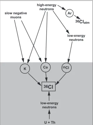
Cette th`ese porte essentiellement sur le radionucl´eide 36Cl. Quatre types de r´eaction entraˆınent la production de 36Cl in situ dans une roche (e.g. Gosse and Phillips, 2001; Schimmelpfennig et al., 2009, Fig. 1):

1. A la surface, le 36Cl est principalement produit par des r´eactions de spallation entre des neutrons de haute ´energie et des ´el´ements cibles, Ca, K, Ti et Fe.

2. La capture des muons n´egatifs lents par le40Ca et le39K entraˆıne une production de 36_{Cl qui devient pr´edominante en profondeur.}

3. La capture de neutrons de faible ´energie (thermique et ´epithermique) par le 35Cl entraˆıne la formation de36Cl.

4. Une production du 36Cl non-cosmog´enique est dˆue `a la capture de neutrons ra-diog´eniques de faible ´energie par le 35Cl form´es suite `a la fission de 238U et `a la d´ecroissance radioactive de l’U et du Th.

L’occurrence de ces r´eactions d´epend 1- du flux de particules cosmiques qui atteint la surface terrestre et 2- de la composition chimique de l’´echantillon, c’est-`a-dire de sa concentration en ´el´ements cibles. Or, le rayonnement cosmique est variable dans l’espace et dans le temps. La production de 36Cl varie donc en fonction de la latitude, de l’altitude et ´egalement en fonction des variations temporelles du champ magn´etique. Pour int´egrer ces variations dans le taux de production correspondant au site ´etudi´e, on calcule pour chaque site un facteur d’´echelle (”scaling factor”). Les mod`eles qui pr´edisent ces variations et sur lesquels se basent ces calculs (e.g. Stone, 2000; Dunai, 2001; Lifton et al., 2005; Desilets et al., 2006b) sont encore en discussion. Par ailleurs, la production in situ d´ecroˆıt exponentiellement avec la profondeur avec une production maximale dans le premier m`etre (e.g. Fig. 1.12).

En l’absence d’´erosion et de pr´e-exposition, la concentration du 36Cl s’accumule en suivant cette ´equation:

N36(z, t) = Ptotal(z) (1 − exp−λ36t)/λ36 (1) Avec Ptotalle taux de production total int´egrant toutes les r´eactions, et qui d´epend de la profondeur z, t le temps d’exposition et λ36 la constante de d´esint´egration (ln2/λ36 = t1/2 avec t_1/2 la demie-vie 301 ka). Cette concentration augmente avec le temps d’exposition jusqu’`a atteindre l’´etat stationnaire, en g´en´eral apr`es une exposition d’environ 3 `a 4 demie-vie (Fig. 1.1). Cet ´etat est atteint lorsque la production du 36<sub>Cl est contrebalanc´ee par</sub> sa perte par d´ecroissance radioactive. Lorsqu’on tient compte des diff´erents processus qui influent sur l’accumulation du 36<sub>Cl dans un ´echantillon, le taux de production total en</sub> nombre d’atomes par gramme de roche par an sur une ´epaisseur connue et situ´e `a une profondeur connue est :

Ptotal(z) = Sel,sFsQsPs(z)+Sel,sFn(QethPeth(z)+QthPth(z))+Sel,µFµ−Qµ−Pµ−(z)+Pr (2) Les indices correspondent au type de r´eaction, s pour spallation, n pour capture des neutrons de faible ´energie, eth pour capture des neutrons ´epithermaux, th capture des

neutrons thermaux, µ− pour la capture des muons n´egatifs lents, et r pour la production radiog´enique. Px est la production de 36Cl r´esultant du type de r´eaction x et d´ependant de la composition chimique de l’´echantillon. Qx est le facteur int´egrant la production sur l’´epaisseur de l’´echantillon. Sel,s et Sel,µ− sont les facteurs d’´echelle qui int`egrent les effets sur l’altitude et la latitude ainsi que les variations temporelles du champ magn´etique pour les r´eactions de spallation (s) et la capture muonique (µ−). Fx int`egre les corrections li´ees `

a tout effet d’´ecrantage (topographie, g´eom´etrie, couverture neigeuse, ect. avec 0 < Fx < 1 et si Fx = 1 pas d’´ecrantage).

Les ´equations 1 et 2 peuvent donc permettre de calculer un ˆage d’exposition d’un ´

echantillon dont on connaˆıt la latitude, l’altitude, les facteurs d’´ecrantage, son ´epaisseur, sa profondeur et dont on a mesur´e tr`es pr´ecis´ement la concentration en36Cl et en ´el´ements cibles (35Cl, Ca, K, Ti et Fe). L’ˆage apparent, c’est-`a-dire en consid´erant une ´erosion nulle et sans pr´e-exposition, est donc :

texpo=

−ln(1 − N_meas λ36/Ptotal)

λ36 (3)

Afin d’obtenir un ˆage d’exposition exact, il est donc essentiel de bien contraindre les taux de production de r´ef´erence. Ces taux de production sont traditionnellement normalis´es `

a un point g´eographique de r´ef´erence qui est le niveau de la mer et les hautes latitudes (SLHL). Or, les taux de production propos´es actuellement dans la litt´erature pour le36Cl montrent des divergences importantes. Celui par spallation du Ca diverge jusqu’`a 46% (Stone et al., 1996; Swanson and Caffee, 2001), et celui par spallation du K diverge jusqu’`a 53% (Zreda et al., 1991; Swanson and Caffee, 2001).

Le projet CRONUS-Europe - Marie Curie Research Training Networks a pour but de contraindre les taux de production et autres param`etres essentiels pour l’utilisation des isotopes cosmog´eniques. C’est dans ce cadre que j’ai effectu´e ma th`ese avec pour objectif de calibrer les taux de production du 36Cl par spallation du Ca et du K, de fa-ciliter l’application de ce nucl´eide `a la quantification des processus superficiels et d’effectuer une inter-calibration des taux de production du 36Cl avec ceux de l’3He et du 21Ne cos-mog`eniques le long d’une transect altitudinal.

Entre autres, nous avons cherch´e `a r´epondre aux questions suivantes :

Pourquoi les taux de production pour le 36Cl montrent une telle divergence ? Quelles sont les valeurs les plus proches de la r´ealit´e pour les taux de production par spallation du Ca et du K ? Quelle est l’influence des facteurs d’´echelle et de leurs incertitudes sur la calibration des taux de production ?

Par ailleurs, la production du 36Cl `a partir du 35Cl est difficile `a param´etrer dˆu `a la distribution complexe des neutrons de faible ´energie `a la limite entre l’atmosph`ere et la roche. Les calculs de production du 36Cl pour un ´echantillon riche en ´el´ement cible 35Cl (e.g. > ∼ 20 ppm dans un basalte) sont donc rendus complexes du fait des incertitudes li´ees `a la valeur du flux de neutrons de faible ´energie et des param`etres qui influent sur ce flux tels qu’une fine couche d’eau ou de neige.

Quel est l’impact des incertitudes inh´erentes `a cette source de production sur la cali-bration des taux de production par spallation ?

Jusqu’`a pr´esent, l’utilisation du36Cl pour quantifier les processus superficiels ´etait sou-vent affect´ee d’incertitudes li´ees aux diff´erents taux de production publi´es et semblait plus compliqu´ee que d’autres cosmonucl´eides comme le 10Be ou le26Al `a cause des sources de production nombreuses et sp´ecifiques `a ce nucl´eide. Il apparaˆıt donc n´ec´essaire de clarifier et de d´ecrire de fa¸con d´etaill´ee les diff´erentes sources de production, leurs incertitudes et leurs domaines d’application. De plus, une feuille de calcul simple permettant la d´etermination des ˆages d’exposition et des taux d’´erosion et int´egrant de fa¸con exacte et pr´ecise toutes les r´eactions de production du 36Cl et applicable `a tout type de roche paraˆıt aujourd’hui indispensable.

Cette th`ese vise donc `a combler ces lacunes pour, d’une part, am´eliorer la justesse des taux de production du 36Cl par spallation, et d’autre part faciliter l’application du 36_{Cl `a la quantification des processus superficiels en proposant une strat´egie pour r´eduire} les incertitudes et en fournissant une feuille de calcul simple pour l’application de cette m´ethode.

cosmog´enique in situ et leur variabilit´e dans l’espace et dans le temps, 2- les m´ethodes utilis´ees pour l’´echantillonage, pour la pr´eparation des ´echantillons, y compris un nou-veau protocole chimique applicable `a tout type d’´echantillon silicat´e, et pour les mesures analytiques, et 3- la description de la nouvelle feuille de calcul pour d´eterminer des ˆages d’exposition et des taux d’´erosion `a partir du 36Cl.

Les r´esultats principaux qui font l’objet d’articles soit publi´e soit en cours de publication dans des revues de rang A sont pr´esent´es dans les chapitres 4, 5 et 6, et sont r´esum´es ci dessous.

D´etermination des sources du 36_{Cl dans des roches basaltiques :}

Implica-tions pour la calibration des taux de production.

Pour expliquer les divergences dans les taux de production du 36Cl propos´es actuellement dans la litt´erature plusieurs sources d’erreur peuvent ˆetre ´evoqu´ees `a savoir (1) l’ˆage du site de calibration ind´ependamment d´etermin´e, (2) les facteurs d’´echelle, (3) la composition des roches utilis´ees, (4) le protocole chimique adopt´e et (5) des m´ecanismes de production non consid´er´es. Alors que Phillips et al. (2001) et Zreda et al. (1991) d´erivent leur taux de production de diff´erents types de roches totales, Stone et al. (1996) et Evans et al. (1997) ont travaill´e sur des min´eraux s´epar´es. A partir de cette observation, nous avons entrepris de tester si ces diff´erences pouvaient expliquer les divergences dans les taux de production. Dans le but d’identifier toutes les sources du 36<sub>Cl dans la roche, nous avons men´e des</sub> exp´eriences de lixiviation et de dissolution successive sur des ´echantillons pr´elev´es sur des coul´ees basaltiques de l’Etna. Les caract´eristiques pahoehoe de ces coul´ees indiquent que l’´erosion est n´egligeable, et les concentrations en 3He cosmog´enique et les ˆages K-Ar sont connus (Blard et al., 2005). Nous avons travaill´e sur des fractions comprises entre 140 et 1000 µm, sur roche totale et sur des plagioclases. Apr`es un premier lessivage dans l’HNO3 dilu´e, les ´echantillons ont ´et´e progressivement dissous en 6 `a 8 ´etapes avec des quantit´es limit´ees d’un m´elange de HF et d’HNO3. Pour chaque ´etape, les concentrations en36Cl et en Cl ont ´et´e d´etermin´ees par spectrom´etrie de masse par acc´el´erateur au LLNL (Figs. 4.3 and 4.3), alors que les concentrations des ´el´ements cibles Ca, K, Fe et Ti ont ´et´e d´etermin´ees au SARM (Fig. 4.5).

Les r´esultats de ces exp´eriences montrent que (1) les concentrations tr`es ´elev´ees en chlore des roches totales (5000 - 300 ppm) entraˆınent une surestimation de l’ˆage d’exposition d’environ 30% par rapport `a l’ˆage attendu (Fig. 4.6), et (2) au contraire, la proc´edure de lixiviation et de d´econtamination est efficace sur les plagioclases apr`es 20% de dissolution avec des concentrations en chlore faibles. Les ˆages d’exposition obtenus sont en accord avec ceux attendus.

Nous avons pu ´ecarter une possible contamination par du36Cl atmosph´erique ou mag-matique qui pourraient ˆetre en partie responsable de ces diff´erences.

Il est donc probable que les divergences dans les taux de production du 36Cl publi´es soient li´ees `a la forte teneur en Cl dans certaines des roches utilis´ees pour les calibrations. En effet, nous pouvons constater que par exemple le taux de production par spallation du Ca publi´e par Phillips et al. (2001) calibr´e avec des roches silicat´ees riches en Cl est presque 30% plus ´elev´e que celui publi´e par Stone et al. (1996) qui ont utilis´e des min´eraux avec de faibles teneurs en Cl. La production du 36Cl `a partir du35Cl est en effet sensible `a des facteurs externes tels qu’une fine couche d’eau qui peuvent maximiser cette production, ces effets sont difficilement quantifiables et encore peu connus (Phillips et al., 2001; Masarik et al., 2007).

Ces r´esultats sont pr´esent´es dans le chapitre 4 et publi´es dans Quaternary Geochronology (Schimmelpfennig et al., 2009).

Par ailleurs, nous avons con¸cu une feuille de calcul Excel , publi´ee dans l’articleR Schimmelpfennig et al. (2009), qui permet de d´eterminer des ˆages d’exposition et des taux d’´erosion `a partir des mesures en 36Cl pour tout type de roche, situ´ee `a la surface ou en profondeur. Cette feuille permet ´egalement de calculer pr´ecis´ement les diff´erentes contributions dans la production de36Cl, c’est-`a-dire connaˆıtre de fa¸con pr´ecise tous les ter-mes qui sont dans l’´equation 2 et contraindre les incertitudes sur les diff´erents param`etres. Toutes les r´eactions qui engendrent la production du 36Cl y sont int´egr´ees. Cette feuille, facile d’utilisation, permet une visibilit´e de tous les param`etres rentrant dans le calcul ainsi que des incertitudes associ´ees. Son utilisation et sa fonctionnalit´e sont d´etaill´ees dans le chapitre 3.

Calibration des taux de production du 36Cl `a partir de la spallation du Ca et du K

Une des difficult´es majeures de la calibration des taux de production du 36Cl est de con-traindre les proportions relatives des diff´erentes sources de production qui d´ependent de la composition chimique de l’´echantillon et particuli`erement de sa concentration en chlore. Pour surmonter cette difficult´e, il convient de travailler sur des min´eraux s´epar´es qui nous permettrons d’isoler la source de production `a calibrer, c’est ce que nous avons montr´e dans le chapitre 4 (Schimmelpfennig et al., 2009). Nous avons donc travaill´e sur des min´eraux riches en Ca et K, contenant tr`es peu de chlore pour calibrer les taux de production du 36_{Cl par spallation du Ca et du K.}

Des plagioclases riches en Ca ont ´et´e s´epar´es `a partir de roches basaltiques de 4 coul´ees provenant du Mt Etna (38◦N, Italie), et des sanidines riches en K ont ´et´e s´epar´es `a partir d’une trachyte d’une coul´ee pr´elev´ee sur le volcan Payun-Matru (36◦S, Argentine). Au total, 13 ´echantillons ont ´et´e pr´elev´es sur les 5 coul´ees dont leur ˆage a ´et´e d´etermin´ees de fa¸con ind´ependante entre 0.4 and 32 ka. Les altitudes des sites d’´echantillonnage au Mt. Etna sont entre 500 et 2000 m et de ceux au Payun Matru entre 2300 et 2500 m. Les facteurs d’´echelle correspondant ont ´et´e calcul´es en utilisant 5 diff´erents mod`eles propos´es dans la litt´erature parmi lesquels quatre incluent les variations du champ magn´etique. Ces facteurs d’´echelle montrent des diff´erences significatives entre les 5 mod`eles avec des ´ecarts entre mod`eles allant jusqu’`a 23% pour les ´echantillons du Mt. Etna et jusqu’`a 7% pour les ´

echantillons du Payun Matru.

En combinant et modifiant les Eqs. 1 et 2, la relation entre la concentration en 36Cl (N36) et les taux de production (SLHL) `a partir du Ca (P RCa) et du K (P RK) que nous cherchons `a d´eterminer a donc pu ˆetre ´ecrite sous la forme:

N36= A × P RCa+ B × P RK+ C (4)

avec A, B et C, des variables qui d´ependent de la composition chimique, de l’ˆage d’exposition, des autres sources de production et des facteurs d’´echelle. Ces variables ont ´

du jeu d’´echantillons, l’´equation 4 a ´et´e adopt´ee et l’ensemble des mesures a ´et´e analys´e statistiquement avec une approche Bayesienne. Cette approche permet de tenir compte d’une fa¸con consistante des incertitudes inh´erentes aux donn´ees utilis´ees notamment sur les ˆages ind´ependants.

Les taux de production d´eriv´es sont les plus bas calibr´es jusqu’`a pr´esent. En appliquant les facteurs d’´echelle calcul´es selon Stone (2000), les taux de production obtenus sont pour P RCade 42.2 ± 4.8 atomes36Cl (g Ca)−1an−1 et pour P RK de 124.9 ± 8.1 atomes36Cl (g K)−1an−1. Ces nouvelles valeurs sont en accord avec les taux de production pr´ec´edemment calibr´es avec des ´echantillons faibles en Cl, notamment avec 48.8 ± 1.7 atomes36Cl (g Ca)−1 an−1, publi´e par Stone et al. (1996), et avec 137 ± 9 atomes36Cl (g K)−1 an−1, publi´e par Phillips et al. (2001).

Les valeurs obtenus avec les 4 autres mod`eles de facteurs d’´echelle sont tr`es proches et comprises dans les barres d’erreur des valeurs ci-dessus. Elles sont pr´esent´ees dans le tableau 5.7 du chapitre 5. Alors que nos donn´ees se r´epartissent sur une p´eriode de temps importante et des altitudes tr`es diff´erentes, les ˆages recalcul´es avec ces nouveaux taux de production sont en accord avec les ˆages ind´ependants quelque soit le mod`ele de facteur d’´echelle choisi. Bien qu’il y ait des diff´erences importantes dans les mod`eles de facteurs d’´echelle, celles ci n’engendrent pas de diff´erences significatives dans les taux de production finaux, parce que: 1- les incertitudes sur nos taux de production sont assez importantes (6 - 10%) et elles r´esultent principalement des incertitudes sur les ˆages ind´ependants, et 2-les divergences entre 2-les diff´erents mod`eles de facteurs d’´echelle ont ´et´e moyenn´ees sur les gammes d’ˆage et d’altitude de l’ensemble de nos donn´ees.

Ce travail est pr´esent´e dans le chapitre 5 et fait l’objet d’une publication que nous pensons soumettre `a Geochimica Cosmochimica Acta.

Inter-calibration des taux de production du 36_{Cl et des gaz rares}

cos-mog´eniques 3_{He et} 21_Ne

Pour d´eterminer l’ˆage d’exposition d’une surface g´eologique, les taux de production utilis´es doivent ˆetre ajust´es `a l’altitude et `a la latitude du site d’´echantillonnage et int´egr´es sur le temps d’exposition. Ceci est dˆu `a la variabilit´e des taux de production avec l’altitude,

la latitude et le temps. Comme discut´e pr´ec´edemment, cette variabilit´e est quantifi´ee `a partir de facteurs d’´echelle eux-mˆemes calcul´es `a partir de mod`eles, encore en discussion. Il est possible que l’inexactitude de ces mod`eles soit en partie responsable des divergences observ´ees dans les taux de production publi´es et par cons´equent entraˆınent des incertitudes sur les ˆages d’exposition (Chapter 5, Balco et al., 2008, 2009).

Ces mod`eles sont g´en´eralement bas´es sur l’hypoth`ese que les r´eactions produisant le nucl´eide, par exemple la spallation, sont soumises `a la mˆeme variabilit´e spatiale et temporelle, ind´ependamment de l’´el´ement cible et/ou du nucl´eide cosmog´enique produit. Cependant, nous savons que les r´eactions qui engendrent la production des cosmonucl´eides ont des seuils ´energ´etiques diff´erents suivant l’´el´ement cible, c’est-`a-dire que la production des divers nucl´eides cosmog´eniques d´epend du spectre ´energ´etique des particules cosmiques (Michel et al., 1995; Lal, 1987, Fig. 6.1). Etant donn´e que l’´energie d’incidence des par-ticules constituant le rayonnement cosmique augmente avec l’altitude et la latitude il est n´ecessaire d’´evaluer si les taux de production des divers cosmonucl´eides ont des variabilit´es spatiales et temporelles diff´erentes. Si c’´etait le cas nous aurions besoin de facteurs d’´echelle individuels associ´es `a chaque nucl´eide ou mˆeme `a chaque r´eaction sp´ecifique `a partir d’un ´

el´ement cible. Gayer et al. (2004) et Amidon et al. (2008) ont sugg´er´e une variabilit´e altitudinale diff´erente pour la production du3He et du 10Be.

Dans le cadre d’une collaboration avec le CRPG, nous avons entrepris de comparer la production du radionucl´eide 36Cl avec celles des nucl´eides stables 3He et21Ne dans des pyrox`enes, riches en Ca, pr´elev´es dans des coul´ees basaltiques le long d’un profil altitudinal (1000 - 4300 m) au Kilimandjaro (Tanzania, 3◦S). Ce travail n’est pas encore totalement abouti puisqu’il sera compl´et´e prochainement par des mesures de ces trois mˆemes isotopes sur des ´echantillons de l’Etna qui suite `a des probl`emes techniques n’ont pas pu ˆetre mesur´es `

a temps pour figurer dans cette th`ese.

Apr`es avoir valid´e un nouveau protocole d’extraction du 36Cl `a partir des pyrox`enes, en mesurant le 36Cl dans des plagioclases co-existant dans un mˆeme ´echantillon, les con-centrations en36Cl,3He et21Ne ont ´et´e d´etermin´ees dans les pyrox`enes.

con-statons aucune d´ependance significative en fonction de l’altitude. Le rapport 21Ne/3He, d´etermin´e dans notre ´etude, est en accord avec ceux d’autres ´etudes (Poreda and Cerling, 1992; Niedermann et al., 2007; Fenton et al., 2009).

Les trois nucl´eides sont ´egalement compar´es en fonction de leurs ˆages d’exposition calcul´es `a partir de leurs concentrations. Cette approche `a pour but de s’affranchir des particularit´es li´ees au nucl´eide 36Cl par rapport aux deux autres nucl´eides, notamment sa d´ecroissance radioactive, sa production par capture des muon n´egatifs lents sur le Ca et sa forte d´ependance avec la composition chimique. L`a encore, il n’est pas observ´e de d´ependance significative avec l’altitude. Cependant il conviendra de tester `a l’avenir une eventuelle d´ependance entre des nucl´eides qui ont des spectres ´energ´etiques plus diff´erents tels que le Ca et le K pour la production par spallation du 36Cl.

Ce travail est pr´esent´e dans le chapitre 6 de cette th`ese.

Conclusion

Les r´esultats de cette th`ese contribuent consid´erablement `a l’am´elioration des aspects m´ethodologiques et analytiques du nucl´eide cosmog´enique36Cl. La mise en ´evidence d’une surestimation des taux de production pr´ec´edemment publi´es avec des ´echantillons `a fortes teneurs en chlore montrent que toutes les diff´erentes sources de production du36Cl doivent ˆ

etre toutes int´egr´ees et consid´er´ees de fa¸con rigoureuse et d´etaill´ee pour obtenir des ˆages d’exposition coh´erents et valables.

Les nouveaux taux de production par spallation du Ca et du K propos´es dans cette ´

etude sont en accord avec les taux pr´ec´edement obtenus avec des ´echantillons faibles en Cl. Ceci permet, d’une part, de reconcilier les pr´ec´edentes calibrations faites et ouvre ainsi la porte `a des d´eterminations d’ˆages d’exposition mieux contraintes et, d’autre part, de mettre en ´evidence les difficult´es et les incertitudes inh´erentes `a l’utilisation d’´echantillon riche en Cl du fait du flux de neutrons thermiques peu contraint et sensible `a divers param`etres encore difficilement quantifiables.

General introduction 7

1 The principles of surface exposure dating with terrestrial cosmogenic

nuclides (TCN) 15

1.1 The application of terrestrial cosmogenic nuclides and their limitations . . . 15

1.2 Cosmic radiation . . . 21

1.2.1 Primary and secondary radiation . . . 22

1.2.2 Effect of the geomagnetic field . . . 24

1.2.3 Cosmic ray particle cascade in the atmosphere . . . 25

1.3 In-situ nuclear reactions and TCN production . . . 27

1.3.1 TCN production by fast neutrons (spallation) . . . 28

1.3.2 TCN production by muons . . . 29

1.3.3 TCN production by thermal and epithermal neutrons . . . 32

1.3.4 Total site-specific TCN production and controlling factors . . . 36

1.3.5 Total TCN concentrations in samples with simple and complex ex-posure history . . . 41

1.3.6 Production of 36_{Cl . . . . 44}

1.3.7 Production of 3He . . . 52

1.3.8 Production of 21Ne . . . 54

1.4 TCN production rates in space and time . . . 55

1.4.1 Five different scaling methods . . . 57

2 From sampling to TCN concentrations: Material and methods 79

2.1 Sampling strategies for calibration of production rates . . . 79

2.2 Physical sample preparation . . . 87

2.3 Measuring 36Cl . . . 92

2.3.1 From sample material to AgCl targets: Chemical 36Cl extraction from silicate rocks . . . 92

2.3.2 From AgCl targets to isotope ratios: 36Cl measurement by Acceler-ator Mass Spectrometry . . . 105

2.3.3 From isotope ratios to36Cl and Cl concentrations: 36Cl Data analysis 110 2.4 Measuring 3He . . . 116

2.4.1 3_{He by Noble Gas Mass Spectrometry . . . 116}

2.4.2 3He Data analysis . . . 119

3 From 36Cl concentrations to surface exposure ages and erosion rates: A new Excel calculation spreadsheet 123 3.1 Particularities of the new 36Cl calculator . . . 124

3.2 What can we do with it? . . . 125

3.3 How to use it? . . . 126

4 Sources of in-situ 36Cl in basaltic rocks. Implications for calibration of production rates 139 4.1 Introduction . . . 141

4.2 Methods . . . 144

4.2.1 Sampling sites and sample description . . . 144

4.2.2 Sample preparation and sequential 36Cl extraction . . . 146

4.2.3 Measurements . . . 149

4.3 In-situ 36_{Cl production mechanisms and calculations . . . 153}

4.4 Results . . . 159

4.5 Discussion . . . 168

5 Calibration of cosmogenic 36Cl production rates by spallation of Ca and K on samples from Mt. Etna (38◦ N, Italy) and Payun Matru (36◦ S,

Argentina) 181

5.1 Introduction . . . 182 5.2 Previous production rate studies . . . 187 5.3 Methodology . . . 190 5.3.1 Sampling strategy and site descriptions . . . 190 5.3.2 Physical and chemical sample preparation . . . 196 5.3.3 Chemical measurements . . . 201 5.4 Production rate calibration approach . . . 202 5.4.1 Calculated in-situ 36Cl production . . . 202 5.4.2 Scaling methods . . . 206 5.4.3 Bayesian statistical approach . . . 213 5.5 Results and discussion . . . 218 5.5.1 New spallation production rates from Ca and K . . . 218 5.5.2 Comparison to previous published production rates . . . 221 5.5.3 Recalculated36Cl ages of the Etna and Payun Matru lava flows . . . 224 5.6 Conclusions . . . 228

6 Determination of relative cosmogenic production rates for3He,21Ne and 36_{Cl at low latitude (3}◦ _{S), along an altitude transect on the SE slope of}

the Kilimanjaro volcano (Tanzania) 233

6.1 Introduction . . . 234 6.2 Geological setting and sampling . . . 237 6.3 Sample preparation, 36Cl, 3He and 21Ne measurements and compositional

analysis . . . 238 6.3.1 Physical sample preparation . . . 238 6.3.2 Chemical 36Cl extraction and measurement . . . 241 6.3.3 Noble gas measurements . . . 242 6.3.4 Major and trace elements . . . 244

6.4 Noble gas data analysis . . . 244 6.4.1 Determination of cosmogenic3He and 21Ne concentrations . . . 244 6.5 Approaches to TCN cross-calibrations . . . 255 6.6 Comparison with other cross-calibrations . . . 267 6.7 Conclusions . . . 268

General conclusions 273

Appendices 281

A Total in-situ 36_{Cl production calculations 281}

A.1 Cosmogenic 36Cl production by spallation of Ca, K, Ti and Fe . . . 283 A.2 Cosmogenic 36_{Cl production by capture of low-energy neutrons... . . 283} A.2.1 Epithermal neutrons . . . 283 A.2.2 Thermal neutrons . . . 287 A.3 Cosmogenic 36Cl production by direct capture of slow negative muons on

40_{Ca and}39_{K . . . 290} A.4 Radiogenic36Cl production . . . 291 A.5 Sample thickness integration factors . . . 292 A.6 Eroded surfaces . . . 293

B Spreadsheet for in situ 36Cl production calculations 297

C Supplementary information for Chapter 5 299

D Supplementary information for Chapter 6 303

The use of terrestrial cosmogenic nuclides (TCN) has revolutionized Earth surface sciences over the last decade by their capacity to quantify geological surface processes. The unique-ness of these nuclides lies in their property of being produced in the top few meters of the lithosphere during exposure to cosmic radiation. Secondary cosmic ray particles that bombard the Earth’s surface interact with certain target elements in the rock producing long-lived radionuclide (10Be, 26Al, 14C and 36Cl) and stable noble gas isotopes (3He and 21_{Ne) that usually do not exist in the rock or only in very small quantities.}

A rock that is suddenly exposed at the surface accumulates an inventory of such cos-mogenic nuclides as time passes by. Hence, the nuclide concentration is a measure of how long the rock has been exposed to cosmic rays, which allows dating the event that led to the exposure of the rock. With the knowledge of the nuclide concentration and of the rate, at which nuclide is produced at the sample site, the exposure duration can be calculated, ignoring for the moment radioactive decay, by the general relationship:

Exposure time = TCN concentration / Local production rate

The challenge of measuring the extreme low level concentrations of TCN with high precision was overcome in the early 1980’s by the groundbreaking improvements in Accel-erator Mass Spectrometry (AMS) and in high sensitivity Noble Gas Spectrometry. Since that time the application of the surface exposure dating method has been steadily in-creasing. However, the accuracy of exposure ages does not only depend on the analytical measurability of the nuclides but also on the accurate knowledge of the mentioned TCN production rates.

funda-mental questions are: how many atoms of the nuclide are produced per g of target material per year? and how does this production rate vary in space and time?

Production rates are experimentally calibrated with geological samples from surfaces that have simple exposure histories and that have been dated accurately and precisely by independent methods. Since such surfaces are rare, globally valid reference production rates are calculated by normalizing calibration sites to a virtual reference position at sea level and high latitude (> 60◦), hereafter SLHL, by accounting for the spatial and temporal variability of the production rates. This variability is primarily due to the varying shielding effect of the geomagnetic field and of the atmosphere on the cosmic radiation and is as such mainly a function of the altitude and the latitude of the sample site. The quantification of this variability is made possible by scaling models that provide methods to calculate scaling factors (e.g. Lal, 1991; Dunai, 2001; Lifton et al., 2005). These scaling factors allow extrapolating SLHL production rates to any geographic position and vice versa.

However, SLHL production rates of most of the TCN, calibrated at different locations by different investigators can differ considerably from each other, in the case of36Cl by up to 50% (e.g. Stone et al., 1996; Swanson and Caffee, 2001). Moreover, numerous existing scaling models yield scaling factors that diverge significantly at some geographic positions. The TCN surface exposure dating method can therefore not yet guarantee a satisfactory accuracy as other geochronometers such as radiocarbon or argon-argon dating.

The European project CRONUS-EU, a Marie Curie Research Training Network, had the objective to better constrain TCN production rates and their variability in space and time as well as other parameters related to the systematics of TCN. In addition to the experimental determination of production rates with geological samples, artificial targets and theoretical modeling were used as approaches. This PhD study, funded by CRONUS-EU, focuses mainly on the experimental calibration of 36_{Cl production rates and the use} of this radionuclide for surface exposure dating.

Four production pathways are responsible for the in situ production of36Cl (Fig. 1):

reactions on the target elements Ca and K, and to a lesser degree on Ti and Fe. 2. A minor production pathway at the surface is the capture of slow negative muons by

40_{Ca and}39_{K. It becomes important at greater depths.}

3. The capture of low-energy (thermal and epithermal) neutrons by 35Cl leads to the production of 36Cl, mainly dependent on the Cl content in the sample.

4. A non-cosmogenic production of36_{Cl is due to slowed down radiogenic neutrons that} form during the spontaneous fission of 238U and (α,n)-reactions on light elements, where the α-particles are produced during U and Th decay.

low-energy neutrons high-energy neutrons slow negative muons 36_Cl 35_Cl Ca K U + Th low-energy neutrons Ar 36_Clatm

Figure 1: Schema of production reactions for 36_{Cl in rock (shaded part) and in the atmosphere}

(white part). Not illustrated are Ti and Fe, which are also target elements for 36_{Cl production}

by interaction with high-energy neutrons (spallation). In addition to in situ production reactions, mentioned in the text,36_{Cl is also produced in the atmosphere by spallation of Ar.}

36_{Cl is often used for surface exposure dating of limestone, since it is currently the} only TCN that can be measured in this rock type and its target element Ca is abundant

in limestone. For cristalline rocks or quartz-containing sediments other nuclides are often preferred due to their simpler and better constrained production systematics. However, in situ 36Cl has the advantage that its chemical extraction is apparently possible from any rock and mineral type that contain at least one of its target elements (Ca, K, Ti, Fe), in contrast to the other TCNs, which are restricted e.g. to quartz in the case of 10Be and 14C or to mafic minerals (olivine and pyroxene) in the case of 3He due to certain chemical behaviors of these nuclides. In addition to limestone, 36Cl is routinely extracted from silicate whole rock and feldspars. Other minerals, such as Ca-rich mafic minerals (e.g. pyroxene) and K-rich felsic minerals (e.g. muscovite) have still to be validated to be suitable for reliable 36Cl extraction.

Also, 36Cl is potentially very well suited to study complex exposure histories such as those involving erosion during exposure or the sudden burial of a surface that was exposed before. For this kind of problem, the approach usually consists in measuring two nuclides in the same sample. The principle is based on the different production and decay rates of the two nuclides, which lead to unique TCN concentration ratios that can be assigned to certain exposure histories. 36Cl has a high potential for this approach due its production systematics that differ essentially from those of the other nuclides.

However, as a matter of fact, none of the 36Cl production rates from its divers target elements is well constrained. The so far published SLHL spallation production rates from Ca differ by up to 46% (Stone et al., 1996; Swanson and Caffee, 2001), and those from K by up to 53% (Zreda et al., 1991; Swanson and Caffee, 2001).

Why have the production rates from spallation of Ca and K such high discrepancies? and what are the valid production rate values? What is the influence of the scaling factors and their inaccuracies in production rate cali-brations?

Also, the production pathway due to capture of low-energy neutrons is difficult to parameterize due to the complex distribution of the low-energy neutrons at the rock/air boundary and due to its dependency on many environmental factors (e.g. Phillips et al., 2001). This makes the calculations difficult, if the target element35Cl is abundantly present

in the sample.

What is the impact of this difficulty, when having high Cl contents in the samples, on the calibration of spallation production rates and how can we avoid propagating the related uncertainties into the spallation production rates?

A simple and comprehensible calculator to routinely compute36Cl production from the various reactions and36Cl exposure ages from rocks with any composition has been lacking up to now. Quantifying surface processes with 36Cl can therefore be a great challenge, if the investigator is not familiar with these issues. As a consequence, the use of 36Cl is generally avoided and other nuclides are preferred.

How can we facilitate the use of 36Cl for exposure age and erosion rate determinations? Which types of rock are most appropriate for the use of 36Cl in quantifying surface processes? How can we guarantee that also non-experts account correctly for all 36Cl production pathways?

In summary, improvements in the accuracy of the36Cl production rates, strategies for reducing uncertainties in exposure ages and erosion rates and the supply of an easily usable means to calculate 36Cl exposure ages will facilitate the use of this promising cosmogenic nuclide and thus significantly broaden the possibilities in surface exposure dating.

This PhD study aims at advancing in these issues. The first three chapters present

1) the principle of TCN production and its variation in space and time,

2) the methods used for sampling, physical and chemical sample preparation, measure-ments and all analytical uncertainties, including a new chemical protocol for36Cl extraction from silicate rock types, and

3) the description of a new36Cl calculator for the determination of exposure ages and erosion rates from any rock type in which36Cl has been measured.

Chapter 4 deals with the understanding of why the existing calibrated production rates diverge so much. The objective is to pave the way for a higher accuracy in a next calibration attempt. Since in previous calibration studies either different kinds of whole

rock or separated minerals were used, we assumed that the discrepancies in the resulting production rates could be related to the chemical differences of these two kinds of target materials. Therefore, 36Cl exposure ages determined from basaltic whole rock and from Ca-feldspars separated from the same rock are compared with the exposure age of the lava determined independently by K-Ar dating to investigate which type of target mate-rial yields the more reliable result. This chapter is accompanied by a detailed review of the theoretical bases for the calculation of 36Cl in any rock type with any composition. It is published in the journal Quaternary Geochronology together with the new Excel R spreadsheet for 36Cl calculations.

Chapter 5 presents a new calibration of 36Cl production rates from spallation of the target elements Ca and K, taking into account the results of the first part of this PhD study. For this purpose, Ca- and K-feldspars low in Cl were separated from five basaltic lava surfaces, whose exposure ages are independently known. The samples were taken at the volcanoes Mt. Etna (Sicily) and Payun Matru (Argentina). The SLHL production rates are determined from the sample set consisting of 20 36Cl measurements by using a Bayesian statistical method accounting for all major uncertainties in the data set.

Chapter 6 of this PhD deals with the comparison of the concentrations of the three cosmogenic nuclides36_Cl,3_{He and} 21_{Ne in pyroxene phenocrysts from lava samples taken} over an altitude transect between 1000 and 4300 m at Kilimanjaro (Tanzania). The objec-tive of this cross-calibration is to investigate if these three nuclides feature different altitude dependences in their production rates, which could help understanding why the existing scaling methods still fail to describe accurately the spatial variability of TCN production rates.

In addition, this last study aims at confirming the use of Ca-rich pyroxene for the successful extraction of 36Cl, which has, to our knowledge, never been attempted before. This method is validated by measuring 36Cl in cogenetic Ca-feldspar minerals separated from the same sample as the pyroxene.

The principles of surface exposure

dating with terrestrial cosmogenic

nuclides (TCN)

1.1

The application of terrestrial cosmogenic nuclides and

their limitations

Development of the TCN dating method. In-situ terrestrial cosmogenic nuclides (TCN) are widely used for surface exposure dating in the earth sciences thanks to the rapid improvements in analytical techniques and in the understanding of the TCN sys-tematics (Gosse and Phillips, 2001). This development, however, is quite recent. The first attempt to date a glacially formed surface in a mafic rock with the in-situ cosmogenic nuclide 36_{Cl was performed in 1955 by Davis and Schaeffer (1955). The lack of an} appro-priate analytical technique that allowed measuring the extreme low-level concentrations of cosmogenic radionuclides impeded further studies in this field for three decades. The development and refinement of accelerator mass spectrometry (AMS) in the early 1980s (Elmore and Phillips, 1987; Finkel and Suter, 1993) marked the beginning of the subse-quently fast progressing research field of cosmogenic isotopes in the earth sciences. The long-lived cosmogenic radionuclides now routinely measured by AMS (see Chapter 2.3.2) are10Be,14C,26Al and36Cl. Simultaneously to the refinements in AMS, it became possible for the measurement of the stable cosmogenic nuclide 3He (Kurz, 1986a,b) and later 21Ne (Graf et al., 1991) with conventional mass spectrometry to be applied for surface exposure dating.

The first empirical calibrations of TCN production rates were performed for 10Be and 26_{Al by Nishiizumi et al. (1986), for}3_{He by Kurz (1986b), for}21_{Ne by Poreda and Cerling} (1992) and for 36Cl by Zreda et al. (1991). Also, the development of a standard means to calculate the relative local production rates for any geographic position on earth (Lal, 1991) (Chapter 1.4) facilitated the routine application of TCN for the quantification of landforming processes.

Geologic applications. Surface exposure dating with TCN has become essential in earth science disciplines such as geomorphology, paleoclimatology and active tectonics. Chronological constraints on the timing and rates of environmental changes (glacial history, erosion) and hazard recurrence frequency (landslides, volcanic and seismic activity) have been quantified using TCN (see reviews in e.g. Gosse and Phillips, 2001; Siame et al., 2006; Muzikar et al., 2003).

Time periods datable with TCN. The TCN method is mainly used to date surfaces generated during the quaternary period. Older surfaces have been dated with the stable cosmogenic noble gases 3He and 21Ne, e.g. sediments with pre-Pliocene ages (> 10 Ma) in Antarctica (Schaefer et al., 1999) or in the Atacama Desert (Dunai et al., 2005). The maximum time range that can be covered with TCN dating is, however, mostly limited to the Quaternary by two factors: the half-life, when using a radioactive nuclide, and the preservation of the surface. In contrast to the two stable nuclides3He and21Ne, the buildup of the radioactive nuclides10Be, 14C, 26Al and 36Cl (half-lives in Table 1.1) increases until steady state is reached, which is when the TCN production is in equilibrium with the radioactive decay (3 - 4 half-lives). For example,36Cl has a half-life of 301 ka, so that after 1 Ma exposure a surface is very close to saturation, whereas the half-life of 10Be is 1.39 Ma (Chmeleff et al., 2009; Korschinek et al., 2009, it has for a long time considered to be about 1.5 Ma), meaning that the saturation limit is reached much later (Fig. 1.1). This generalization is, however, only true for non-erosion conditions.

As the rock surface is exposed to cosmic radiation, it is usually also subject to erosion. Erosion affects the TCN concentration in a surface sample, mostly lowering the concen-tration compared to the non-erosion condition (see Fig. 1.1). The older the surface the

higher this effect. There are then two unknowns, the exposure time and the erosion rate (Lal, 1991). 2 4 6 8 10 12 10 6 atoms 36Cl/(g sample) 0

exposure time (Ma)

Accumulation of 10_{Be and} 36_{Cl in function of time and erosion rate}

no erosion 1 mm/ka 5 mm/ka 10 mm/ka

B

_Cl

t

= 301 ka

exposure time (Ma)

10 6 atoms 10Be/(g sample)

A

_Be

t

= 1.39 Ma

Figure 1.1: Accumulation of the radionuclides 10_{Be (A) and} 36_{Cl (B) in a hypothetical surface}

sample in function of time (0 to 3 Ma) and steady erosion rates. 10_{Be concentrations are calculated}

for a quartz sample, and36_{Cl concentrations for a Ca-rich Cl-free plagioclase sample (i.e. production}

from spallation is dominant). In both cases, the sample site is at mid latitude and 2000 m altitude. Due to its shorter half-life, 36_{Cl reaches earlier its equilibrium concentration. The dashed lines in}

(A) demonstrate that the nuclide concentration is lower the higher the erosion rate for the same exposure duration. The dashed lines in (B) illustrate that underestimating or ignoring erosion for a given measured nuclide concentration leads to an apparently younger exposure age.

Exposure age and erosion rate of a surface can be determined simultaneously by com-bining two TCN with different half-lifes. Up to now, this approach has mainly been used

with the nuclides 10Be and26Al, since their production mechanisms are fairly well known and simple and both nuclides can be measured in quartz (e.g. Nishiizumi et al., 1991). However, also 36Cl is potentially very useful for this method due to its relatively short half-life and the variety of its production mechanisms (e.g. Liu et al., 1994; Gillespie and Bierman, 1995).

Another method to constrain the exposure age and erosion rate of a surface is by measuring nuclide concentrations over a certain depth range and using the characteristic depth profile, its shape also depending on the erosion rate and the exposure history (e.g. Siame et al., 2004; Braucher et al., 2009, and see Fig. 1.2). 36Cl is particularly suited for this approach due to its unique vertical distribution if production due to low-energy neutrons is dominant (see Fig. 1.12 and Chapter 3.3 for details).

Figure 1.2: Vertical distribution of 10_{Be in a depth profile for various exposure histories (from}

Gosse and Phillips, 2001): A - One simple and continuous exposure event. B - Gradual erosion at a constant rate. C - The surface is continously aggrading by sedimentation at a constant rate. D - After a continuous period of exposure a former surface (now at ∼200 cm) was suddenly burried; the new surface is now constantly exposed.

restricted to Quaternary surfaces, a drawback of the isotopic stability is that the nuclide clock is never set to zero by decay, so that a more frequent problem is inheritance, initially present amounts of the nuclide inherited from exposure periods prior to that of interest (Bierman, 1994).

The minimum time period that can be dated is mainly controlled by the analytical sensitivity and the non-cosmogenic background concentrations of the respective nuclide. The nuclide quantity in a sample can be too low to be accurately detected by the measure-ment technique (Chapter 2.3.2). In this context the value of the production rate has to be considered because the accumulation of a nuclide in a sample is govered by its production rate: the higher the production rate the faster the accumulation. Of the nuclides men-tioned above, 10Be has the lowest reference production rate (about 5 atoms (g quartz)−1 a−1) and3He has the highest production rate in olivine and pyroxene (about 120 atoms/ (g mineral)−1 a−1). However, the low-level concentrations in a sample might be compensated by extracting the respective nuclide from a larger sample (see Chapter 2.1 for 36Cl). Due to improvements of the sensitivity of the AMS technique, 10Be exposure ages as young as 200 years with 1 σ analytical uncertainties of less than 10% have been recently determined at LLNL-CAMS (Schaefer et al., 2009; Licciardi et al., 2009). In Chapter 5 of this dis-sertation the 36Cl measurement of a 400 year young lava flow is part of the data set for the 36Cl production rate calibration. Its 36Cl concentration has been determined with a 1 σ analytical uncertainty of less than 4% at LLNL-CAMS. Non-cosmogenic background concentrations due to radiogenic, nucleogenic and/or magmatic origin of the nuclide can limit the identification of the cosmogenic component in the case of very young samples. This concerns 3He, 21Ne and 36Cl (Chapters 1.3.6, 1.3.7 and 1.3.8).

Choice of nuclide. When applying the TCN method, the choice of the nuclide depends mainly on the lithology of the rock surface of interest, because TCN production varies in different minerals as a function of their composition. Since cosmogenic nuclides are produced by interaction of secondary cosmic ray particles with certain target elements (Chapter 1.3), they can only accumulate in a sample if at least one of the respective target elements is present. The nuclides 10Be, 26Al and14C are almost always studied in quartz,

Table 1.1: Half-lives of the cosmogenic radionuclides and the mineral phases each TCN is routinely extracted from with the corresponding lithologies.

Nuclide Half-life Mineral phases Type of lithology

3_{He - pyroxene, olivine mafic volcanic rocks}

10_{Be 1.39 Ma quartz magnetic rocks, sandstone, conglomaterates}

14_{C 5.73 ka quartz magnetic rocks, sandstone, conglomaterates}

21_{Ne - quartz, pyroxene,}

olivine

magnetic rocks, sandstone, conglomaterates

26_{Al 720 ka quartz magnetic rocks, sandstone, conglomaterates}

36_{Cl 301 ka calcite, Ca/K-rich} feldspar, whole rock

magnetic rocks, limestone, Mg-carbonate

because Si and O are their most important target elements (for26Al only Si) and because certain characteristics of the nuclides can make it difficult to measure them in other mineral phases.

For example, atmospheric10_{Be, produced in the atmosphere by spallation of O and N,} is highly reactive with mineral surfaces, which therefore require a rigorous decontamina-tion. This atmospheric component is often much larger than the in situ cosmogenic 10_Be component. Kohl and Nishiizumi (1992) measured10Be concentrations in the first leaches of quartz that are two orders of magnitude larger than those measured from completely pu-rified quartz. While quartz can be relatively easily decontaminated from this atmospheric 10_{Be by acid-leaching (Kohl and Nishiizumi, 1992), other minerals that are less resistant} to alteration such as olivine and pyroxene seem to be more problematic (Seidl et al., 1997). Though, 10Be has been successfully measured in mafic minerals (Braucher et al., 2006; Blard et al., 2008). Also, in situ 10Be extraction from carbonates has been unsuccessful until now due to absorption of atmospheric 10Be on clay mineral surfaces (Merchel et al., 2008b). Although the use of 10Be for surface exposure dating is often preferred, because its production systematics are relatively well constrained, its wide use has so far been restricted to lithologies containing quartz.

Also21Ne can be measured in quartz in contrast to3He, which diffuses too rapidly from this mineral and other mineral phases (Brook et al., 1993). 3He is most often measured in

olivine and pyroxene, which bear several of its target elements for spallation reactions in varying stoichiometric ratios (O, Mg, Si, Ca, Fe, Al).

36_{Cl is, besides}10_{Be and}26_{Al, the most used TCN. It is produced by various production} reactions on target elements commonly abundant in many lithologies, most notably Ca, K and Cl. Like 10Be it is also produced in the atmosphere, by spallation of Ar. Cosmic rays produce 3 - 6 × 104 atoms 36Cl cm−2 a−1 in traversing the atmosphere, resulting in atmospheric 36Cl/Cl ratios in the range of 10−15 (near costs) and 10−12 (inland) (Stone et al., 1996, and references herein). In situ cosmogenic 36Cl/Cl ratios are on the order of 10−13 to 10−11. In contrast to 10Be, the chemical decontamination from atmospheric 36_{Cl does not pose a problem due to the hydrophilic behavior of Cl (e.g. Merchel et al.,} 2008a, see also Fig. 2.11). Also, 36Cl does not diffuse from certain minerals, since it is not a gas. It can therefore be measured in any rock material containing at least one of its target elements such as carbonates, Ca- and K-feldspars and mafic and felsic whole rocks. Even minerals without target elements in the crystal lattice, such as quartz, can be used for the extraction of 36Cl, produced from Cl in fluid inclusions (e.g. Bierman et al., 1995). The multiplicity of the 36Cl production reactions, however, is partly responsible for the discrepancies between the calibrated production rates and sometimes renders the interpretation of 36Cl measurements difficult due to high uncertainties in the involved parameters (Chapter 4).

1.2

Cosmic radiation

In situ cosmogenic nuclides are produced by nuclear reactions between particles coming from the cosmos and certain target elements in the rock material. However, before this cosmic radiation reaches the earth’s surface its flux and energy spectrum change as it is ”filtered” through the geomagnetic field and as it passes through the atmosphere. A detailed synthesis of the underlying theory is given in Lal and Peters (1967) and in the review paper Gosse and Phillips (2001).

22

The principles of surface exposure dating with terrestrial cosmogenic nuclides (TCN)

Atmospheric

36

_{Cl/Cl (x 10}

_{) in the USA}

Figure 1.3: Distribution of36Cl/Cl ratios in meteoric deposition in the United States after Bentley et al. (1986) (taken from Moysey et al., 2003).

1.2.1 Primary and secondary radiation

The primary cosmic radiation consists of energetic charged particles, primarily protons (∼85%) and α-particles (∼14%), but also including heavier nuclei and electrons. These particles originate mainly from very energetic processes such as supernova explosions within our galaxy and to a small component outside our galaxy, and are called galactic cosmic radiation. Cosmic ray particles produced during sporadic solar flare events in the sun are referred to as solar cosmic radiation, which is less energetic than the galactic cosmic radiation. Most primary cosmic particles have energies too low to penetrate the earth’s atmosphere and the radii of their spiral trajectories in the earth’s magnetic field tends to channel them to the poles. The influence of the magnetic field on the primary radiation is described in the next section. However, if the particles are sufficiently energetic (1 GeV < E < 1010GeV), they can penetrate into the upper atmosphere, where they produce nuclear desintegrations. The secondary radiation is a product of these interactions between primary radiation and atoms in the atmosphere, resulting in a cascade of particles and reactions (Fig. 1.4). The cosmic ray flux at depth in the atmosphere is composed of primary and

secondary particles.

Figure 1.4: Cascade of secondary cosmic ray particle production in the atmosphere starting with a primary particle penetrating in the upper atmosphere and ending with TCN production in the rock, from Desilets and Zreda (2001). The left part shows the electromagnetic component, dominated by electrons (e) and gamma rays or photons (γ) (low-mass particles that do not contribute to TCN production). The right part shows the hadronic component, dominated by protons (P) and neutrons (N), mostly responsible for TCN production. The middle part shows the mesonic component, here pions (π) are illustrated that decay into muons (µ). Muons have a longer attenuation length than the neutrons and protons (see text).

1.2.2 Effect of the geomagnetic field

The effect of the geomagnetic field on the cosmic radiation, described in this section, is based on Stormer’s theory that considers the Earth as a dipole (Stormer, 1935), meaning that the geomagnetic field intensity (or strength) is constant along a single latitude. In reality, the field strength varies longitudinally, indicating that the geomagnetic field is more complicated than a simple dipole field model (see Chapter 1.4 for more details), which, however does not make invalid the general principle of the here described effects.

Approaching the Earth’s atmosphere, a charged primary’s trajectory is deflected by the terrestrial geomagnetic field. Near the magnetic equator, low-energy primaries are inhibited from penetrating the atmosphere and are deflected away from the Earth. This is because, near the equator, particles must cross the magnetic field lines, while near the poles they can enter the atmosphere parallel to the field lines, which greatly reduces the magnetic shielding effect. Charged primaries with a certain energy, however, can pass through the magnetic field even at low latitudes. In other words, the geomagnetic field imposes a lower limit on the energy of primary cosmic ray particles to enter the upper atmosphere. This shielding effect is usually described by the concept of cutoff rigidity (Rc) of the geomagnetic field, which is a measure for the minimum energy a particle of a given charge must have not to be deflected by the geomagnetic field . The geomagnetic cutoff rigidity depends on the magnetic field strength and is therefore strongly latitude-dependent. Toward higher latitudes, the dipole field lines become steeper, so that the field strength and the threshold rigidity decreases. Near the magnetic poles, at latitudes higher than 60◦, the cutoff rigidity drops below the minimum energy of the primaries required to produce the particle shower in the atmosphere that is responsible for TCN production at the surface of the Earth (next section). The net effect is that a harder (higher average energy) flux penetrates the upper atmosphere at the magnetic equator, and that higher latitudes receive a wider spectrum of energies. TCN production therefore increases with increasing latitude (Fig. 1.5).

Temporal variations in the magnetic field strength only affect the cosmic ray flux below 60◦ latitude. Analogously, the TCN production is affected by the temporal variations