HAL Id: hal-00295223
https://hal.archives-ouvertes.fr/hal-00295223
Submitted on 3 Feb 2003
HAL is a multi-disciplinary open access
archive for the deposit and dissemination of
sci-entific research documents, whether they are
pub-lished or not. The documents may come from
teaching and research institutions in France or
abroad, or from public or private research centers.
L’archive ouverte pluridisciplinaire HAL, est
destinée au dépôt et à la diffusion de documents
scientifiques de niveau recherche, publiés ou non,
émanant des établissements d’enseignement et de
recherche français ou étrangers, des laboratoires
publics ou privés.
derived from 1979-1993 global CTM simulations
F. Dentener, M. van Weele, M. Krol, S. Houweling, P. van Velthoven
To cite this version:
F. Dentener, M. van Weele, M. Krol, S. Houweling, P. van Velthoven. Trends and inter-annual
vari-ability of methane emissions derived from 1979-1993 global CTM simulations. Atmospheric Chemistry
and Physics, European Geosciences Union, 2003, 3 (1), pp.73-88. �hal-00295223�
www.atmos-chem-phys.org/acp/3/73/
Chemistry
and Physics
Trends and inter-annual variability of methane emissions derived
from 1979–1993 global CTM simulations
F. Dentener1, M. van Weele2, M. Krol3, S. Houweling4, and P. van Velthoven2
1JRC, Institute for Environment and Sustainability, I-21020 Ispra (Va), Italy 2KNMI, de Bilt, the Netherlands
3IMAU, Utrecht University, the Netherlands 4MPI Biogeochemistry, Jena, Germany
Received: 6 February 2002 – Published in Atmos. Chem. Phys. Discuss.: 7 March 2002 Revised: 30 September 2002 – Accepted: 11 January 2003 – Published: 3 February 2003
Abstract. The trend and interannual variability of methane sources are derived from multi-annual simulations of tro-pospheric photochemistry using a 3-D global chemistry-transport model. Our semi-inverse analysis uses the fif-teen years (1979–1993) re-analysis of ECMWF meteoro-logical data and annually varying emissions including photo-chemistry, in conjunction with observed CH4concentration
distributions and trends derived from the NOAA-CMDL sur-face stations. Dividing the world in four zonal regions (45– 90 N, 0–45 N, 0–45 S, 45–90 S) we find good agreement in each region between (top-down) calculated emission trends from model simulations and (bottom-up) estimated anthro-pogenic emission trends based on the EDGAR global an-thropogenic emission database, which amounts for the period 1979–1993 2.7 Tg CH4yr−1. Also the top-down determined
total global methane emission compares well with the total of the bottom-up estimates. We use the difference between the bottom-up and top-down determined emission trends to calculate residual emissions. These residual emissions re-present the inter-annual variability of the methane emissions. Simulations have been performed in which the year-to-year meteorology, the emissions of ozone precursor gases, and the stratospheric ozone column distribution are either varied, or kept constant. In studies of methane trends it is most impor-tant to include the trends and variability of the oxidant fields. The analyses reveals that the variability of the emissions is of the order of 8 Tg CH4yr−1, and likely related to wetland
emissions and/or biomass burning.
1 Introduction
Atmospheric methane (CH4) concentrations have more than
doubled since the pindustrial era. This increase has re-sulted in a radiative forcing of about 0.5 Wm−2. Methane is
Correspondence to: F. J. Dentener (frank.dentener@jrc.it)
therefore the most important increasing greenhouse gas af-ter CO2. During the past two decades (from 1978–1998) the
globally averaged methane concentration has increased from about 1520 to 1745 ppbv (Prather et al., 2001). The rate of the methane increase has varied substantially during this period. Values were of the order of 20 ppbv yr−1during the 1970s, a rather constant value of 12 ppbv yr−1 in the 1980s, and al-most zero increase in the years 1992 and 1993 (Lelieveld et al., 1998; Dlugokencky et al., 1998). Over the period 1993 to 1998 the rate of increase was about 5 ppbv yr−1.
A remarkable depression of the methane growth rate oc-curred during 1992 and 1993, which may be attributed to the impact of the eruption of Mt. Pinatubo in June 1991. This eruption has likely caused lower northern latitude wetland emissions (Hogan and Harris, 1994) and changes in the tro-pospheric OH content related to stratospheric ozone deple-tion (e.g. Bekki et al., 1994). The Pinatubo erupdeple-tion clearly showed that the observed methane growth rate and its varia-tions are the result of an imbalance between methane emis-sions (sources) and destruction rates (sinks).
This work attempts to assess the trend and inter-annual variability of methane emissions over the period 1979–1993 by applying a a mass balance approach implemented in a CTM. As an a priori estimate the model uses the natural and anthropogenic CH4emissions evaluated by Houweling
et al. (1999), see Table 1. These emissions do not contain inter-annual variability. The effective CH4 emissions are
calculated from simulations in which the CH4observations
from the NOAA CMDL network are assimilated into the model. We use the results of a set of simulations used previ-ously to study the trends and variability of ozone (O3) during
the same time period (Lelieveld and Dentener, 2000). Here the simulations (including meteorological and photochemi-cal variability) are used to investigate whether (top-down) model calculated CH4emissions and derived trends are
con-sistent with current (bottom-up) knowledge on the tempo-ral and spatial changes in the anthropogenic and/or natutempo-ral
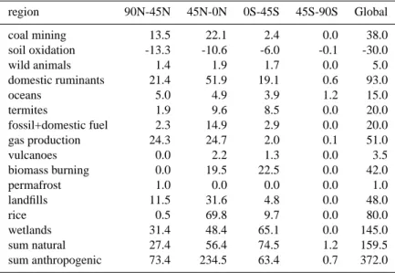
Table 1. Emissions Tg CH4yr−1evaluated by Houweling et al. (1999) used as an a-priori estimate region 90N-45N 45N-0N 0S-45S 45S-90S Global coal mining 13.5 22.1 2.4 0.0 38.0 soil oxidation -13.3 -10.6 -6.0 -0.1 -30.0 wild animals 1.4 1.9 1.7 0.0 5.0 domestic ruminants 21.4 51.9 19.1 0.6 93.0 oceans 5.0 4.9 3.9 1.2 15.0 termites 1.9 9.6 8.5 0.0 20.0 fossil+domestic fuel 2.3 14.9 2.9 0.0 20.0 gas production 24.3 24.7 2.0 0.1 51.0 vulcanoes 0.0 2.2 1.3 0.0 3.5 biomass burning 0.0 19.5 22.5 0.0 42.0 permafrost 1.0 0.0 0.0 0.0 1.0 landfills 11.5 31.6 4.8 0.0 48.0 rice 0.5 69.8 9.7 0.0 80.0 wetlands 31.4 48.4 65.1 0.0 145.0 sum natural 27.4 56.4 74.5 1.2 159.5 sum anthropogenic 73.4 234.5 63.4 0.7 372.0 methane sources.
Bottom-up estimates of the global methane source strength over the past two decades amount to about 500–600 Tg CH4yr−1(Prather et al., 2001). Extensive overviews on
in-dividual methane sources are presented in e.g. Lelieveld et al. (1998). Natural sources consist of high and low lat-itude wetlands, termites, wild animals, oceans, volcanoes and wildfires. Houweling et al. (2000) evaluated the (pre-industrial) annual wetland emissions to be between 130– 194 Tg CH4yr−1, all other natural sources amounting to
about 40–70 Tg. Anthropogenic sources are related to pro-duction and consumption of gas and oil, ruminants, landfills, rice agriculture and biomass burning. Most bottom-up es-timates of the global anthropogenic sources are remarkably similar and amount to 315–350 Tg CH4yr−1(Prather et al.,
2001, and references therein).
The estimates of the latitudinal distributions of the emis-sions by various authors show substantially less consensus. For example, an early study by Fung et al. (1991) distributes the anthropogenic and natural emissions over the Northern and Southern Hemisphere (NH and SH) by a ratio 499 to 144 Tg CH4yr−1. Lelieveld et al. (1998) suggest a NH-SH
ratio of 399 to 123 Tg CH4yr−1. The inverse model results of
Hein et al. (1997) indicate a ratio of 416 to 162 Tg CH4yr−1,
whereas the adjoint inverse model of Houweling et al. (1999) rather calculates 340 and 165 Tg CH4yr−1, for the NH and
SH, respectively. Therefore, there are large uncertainties as-sociated with the individual sources of methane and their ge-ographical and temporal distribution.
What do we know about emission trends? Recently, Dlu-gokencky et al. (1998) analysed the NOAA CMDL CH4
measurements for the period 1984–1996. They suggested that during this period CH4emissions must have remained
almost constant. However, this conclusion strongly depends on the assumption that the global hydroxyl (OH) radical con-centrations also remained constant. At present, this topic is strongly under debate. Prinn et al. (1995) and Prinn and Huang (2001) used methyl-chloroform (MCF) observations to derive an OH trend of 0.0% ± 0.2% yr−1 for the pe-riod 1978–1993. In contrast, using the same observational data-set, but a different statistical analysis technique and as-sumptions on initial pre-1978 conditions, Krol et al. (1998) and Krol et al. (2001) derive a positive OH trend of 0.46 ± 0.6% yr−1. The latter trend estimate is more consistent with the results of the simulations used in this study as well as an independent model study by Karlsd`ottir et al. (2000). In a recent study Prinn et al. (2001) derive a strong positive OH trend for the period 1979–1989 followed by a negative trend in the period 1990–2000.
The global bottom-up estimate of 500–600 Tg CH4yr−1
is roughly consistent with top-down model estimates on the global methane source where global OH is calibrated us-ing observed MCF concentrations (Houwelus-ing et al., 2000). However, these top-down estimates are also associated with large uncertainties of at least 10% (see Sect. 5). In addition, due to the scarcity of measurements it seems at present not possible to determine from the concentration measurement at the surface one unique source/sink configuration (Hein et al., 1997; Fung et al., 1991). In future the availability of isotopic data may help to improve the situation (e.g. Lassey et al., 1993). Also upcoming satellite data measuring tropo-spheric methane columns may improve our knowledge on the geographical and temporal variation of methane sources. This work does not aim to improve the knowledge on the CH4source distributions and strengths, but rather focuses on
The CTM used in this study is described in Sect. 2. Details on the methodology to derive the emission trends for the pe-riod 1979–1993 are given in Sect. 3. This pepe-riod was chosen, since we have a consistent meteorological dataset from the ECMWF-ERA15 dataset, as well as an emission dataset for this period. In Sect. 4 we will present results for 3 different simulations with different combinations of varying meteorol-ogy, emissions and stratospheric ozone boundary conditions. The sensitivity of the method to possible measurement and model errors will be discussed in Sect. 5. Conclusions are presented in Sect. 6.
2 Global chemistry transport model
The global chemistry-transport model TM3 (Heimann, 1995; Houweling et al., 1998; Lelieveld and Dentener, 2000, and references therein) is used in this study at a spatial resolu-tion of 10◦longitude and 7.5◦latitude with 19 vertical
lay-ers. Six-hourly meteorological fields from the ECMWF (Eu-ropean Centre for Medium Range Weather Forecast) ERA15 re-analysis for the years 1979–1993 (Gibson et al., 1997) are utilised. These fields include global distributions for hori-zontal wind, surface pressure, temperature, humidity, liquid water content, ice water content, cloud cover, large-scale and convective precipitation. Tracer advection is simulated with the so-called ‘slopes’ scheme (Russell and Lerner, 1981). Convective tracer transport is calculated with a mass flux scheme that accounts for shallow, mid-level and deep con-vection (Tiedke, 1989). Turbulent vertical transport is calcu-lated by stability dependent vertical diffusion (Louis, 1979). A detailed comparison between simulated and measured Rn222 has indicated that the synoptic scale model transport properties are represented relatively accurately at the applied resolution (Dentener and Crutzen, 1994). Also the compari-son between modelled ozone and several background ozone soundings as presented in Lelieveld and Dentener (2000), revealed a quite satisfactory agreement between model and measurements.
The chemical scheme is based on a modified version of CBM4 that describes the chemistry of CH4-CO-NMHC-NOx
(Houweling et al., 1998) as well as NHx, DMS, SOx
(Den-tener and Crutzen, 1994). In its present form the scheme accounts for 24 photo-dissociation and 67 thermal reactions as well as reactions on aerosols and in clouds. Dry de-position of gases and aerosols is parameterized according to Ganzeveld et al. (1998), and wet deposition according to Guelle et al. (1998). Photolysis frequencies are calculated with the scheme by Landgraf and Crutzen (1998), including the effects of clouds, surface albedo and the overhead ozone column following Krol and Van Weele (1997).
Stratospheric boundary conditions are applied to ozone, methane and nitric acid (HNO3). At levels above 50 hPa
stratospheric ozone is relaxed towards the zonal and monthly mean ozone column measurements by the Total Ozone
Map-ping Spectrometer (TOMS) (McPeters, 1996) using a vertical distribution from an ozone climatology representative for the 1980s (Fortuin and Kelder, 1998). The ozone column above 10 hPa is prescribed. The 3-D ozone variability in the strato-sphere is maintained by simulated transport. Since TOMS measurements are not available for a large part of the year 1993, we apply the 1992 TOMS measurements for 1993.
CH4is destroyed mainly by OH in the troposphere and by
reactions with OH, Cl and O1D in the stratosphere. Since TM3 does not explicitly consider stratospheric reactions, we apply in the stratosphere a methane loss rate varying between 38 and 42 Tg CH4yr−1, based on 2-D model results of Br¨uhl
and Crutzen (1993).
Except for methane (see Sect. 3), yearly anthropogenic emissions of NOx, CO, NMHC, SOx, and NH3 are
di-rectly taken from the emission database developed by Aar-denne et al. (2001). This database, which is based on the widely used EDGAR emission database (Olivier et al., 1999), describes the development of emissions during the period 1890–1990. We used the base years 1970, 1980, 1985, and 1990, and linearly interpolated the results for the years 1979– 1990. Emissions for the period 1991–1993 are obtained by extrapolation of the 1990 emission using CO2emission
statistics obtained from Marland et al. (2000). Natural emis-sions of O3 precursor gases are prescribed as described in
Houweling et al. (1998). The emission data-set does not ac-count for their possible inter-annual variability, with the ex-ception of NOx resulting from lightning discharges, which
is coupled to modelled convection, and therefore lightning NOx emissions show an inter-annual variability of about
0.5 TgN yr−1.
3 Analysis method
We use a relatively simple mass-balance inversion method coupled to a rather complex model of atmospheric transport and chemistry to assess the consistency of the present-day in-formation on methane emissions, atmospheric chemistry and observations. This approach has the advantage over more sophisticated inversion formalisms such as the Green’s func-tion approach or Kalman filtering, that it is easier to imple-ment and computationally less expensive. A disadvantage, however, is a loss of accuracy resulting from a simplified treatment of source-inference rules. We demonstrate by a test with synthetic emissions (see Appendix), that these er-rors are expected to be small on the large temporal and spa-tial scales that we use in this study. Another advantage of our approach is that it advoids cumbersome iterative lineari-sations of this (weakly) non-linear inversion problem. Un-like previous studies, our method guarantees that feedbacks of CH4on OH are accounted for in a consistent way.
There-fore, the use of our simple method, provides an alternative for more conventional inversion methods, for which the real uncertainties are not very well known (compare e.g.
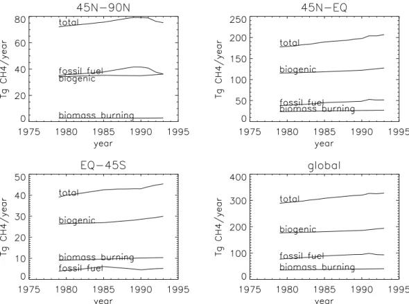
Houwel-Fig. 1. Temporal development of anthropogenic CH4emissions separated for biogenic, fossil fuel related, and biomass burning emissions. Global and 3 world regions.
ing et al., 1999; Hein et al., 1997). For a more comprehensive discussion on this topic we refer to the previous discussion in ACPD (Rayner, 2002; Kaminski, 2002).
As a starting point of the simulations we use the a pri-ori natural and anthropogenic CH4emissions that were
ob-tained from Houweling et al. (1999), see Table 1. The an-thropogenic part of these emissions, is with some small adaptations, consistent with the emissions from the EDGAR database (see below). Note that these a priori emissions do not contain inter-annual variability, and are not representative for a specific year. In a next step the measured concentra-tions are assimilated in the model using the measurements of the NOAA CMDL network in combination with model results (see Sect. 3.2). In order to interpret the methane trends and to determine the inter-annual variability and trend of the methane emissions we calculate so called ‘residual emissions’. These residual emissions are calculated from the difference of the top-down determined yearly methane emissions from a model simulation constrained by observed trends, and the bottom-up estimated time evolution of anthro-pogenic methane emissions from the EDGAR inventory. In this section we present the time evolution in the emission in-ventories and explain our method to calculate emissions from a model simulation and to derive the residual emissions.
3.1 Time evolution of anthropogenic emissions
In Fig. 1 we present the bottom-up estimated yearly anthro-pogenic methane emissions for the period 1979–1993 as adopted from Aardenne et al. (2001). For clarity we have aggregated the detailed 1 × 1 degree data set in four zonal regions (45 N–90 N; 0–45 N; 0–45 S; 45 S–90 S) and three source categories (fossil fuel, biogenic and biomass burning). For comparison Houweling et al. (2000), used in his study emissions of 73.4, 234.5 and 63.4, and 0.7 Tg CH4yr−1
for the anthropogenic emissions in the 4 regions, respec-tively. Natural emissions (including uptake by soils) were 27.4, 56.4, 74.5 and 1.2 Tg CH4yr−1, respectively (see
Ta-ble 1). Since there are no significant anthropogenic emis-sions south of 45 S this region is not included separately in Fig. 1. The fossil fuel emissions encompass all emissions as-sociated with the production and consumption of fossil fuels. Biogenic emissions contain emissions from ruminants, rice-paddies and landfills. Biomass burning emissions include sa-vannah fires, deforestation, waste burning and domestic bio-genic fuel use. At middle and high northern latitudes fos-sil fuel and biogenic emissions are of equal importance. At low latitudes and in the Southern Hemisphere biogenic emis-sions are largest. Although especially biomass burning is known to exhibit a strong inter-annual variation, such
vari-Table 2. NOAA stations used in this work to derive the model trends
Station Code Long Lat Polar Front CTM 2E 66N Cold Bay CBA 162W 55N Mould Bay MBC 119W 76N Barrow BRW 156W 71N Cape Meares CMO 123W 45N Key Biscayne KEY 80W 25N Mauna Loa MLO 155W 19N Cape Kumukahi KUM 154W 19N Guam GMI 144E 13N Ascension Island ASC 14W 8S Tutuila,Samoa SMO 170W 14S South Pole SPO 24W 90S
ations in anthropogenic emissions, other than by economical and demographic developments, are not taken into account in the bottom-up emission estimates. Calculated anthropogenic trends are markedly different in the mid-and-high-latitude Northern Hemisphere, and the rest of the world.
3.2 Boundary conditions for top-down emission estima-tions
For the top-down determination of the methane emissions we performed model simulations covering the period 1979 to 1993. In these simulations the calculated methane mixing ratios are adjusted in the boundary layer, i.e. the first 3 model layers up to 600 m height, using a relaxation time scale of 10 days, to match the model zonal average to a prescribed set of zonally and monthly averaged methane mixing ratios de-rived from and consistent with observations. This timescale was choosen to include synoptic events, without constrain-ing the model too strongly to the measurements. The choice to adjust these three model layers, rather than only the sur-face layer with a thickness of about 60 m, is motivated by the fact that the observational (mostly marine) data-set is proba-bly more representative for a mixed boundary layer than for continental surface layer concentrations. The observational data set consists of the independently determined zonally and monthly averaged methane mixing ratios for the year 1987 (which is in the middle of our modelling period) adopted from the inverse modelling study by Hein et al. (1997). The results of the zonal mean results of this independent inverse modeling study are useful as a constraint as the difference of the observed and calculated concentrations was minimized by their inversion. On top of this field we impose for the period 1984–1993 a trend derived from twelve background stations from the NOAA network for which there is a com-plete record during this time period (see Table 2).
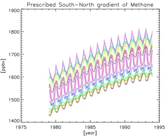
The global annual trend was obtained by equally
weight-Fig. 2. Latitudinal and temporal evolution of prescribed methane volume mixing ratio [ppbv]. Each color represents a different lati-tude, starting from 86 N at the top in steps of 8 degrees.
ing of all stations. This yields a trend that is somewhat biased to the Northern Hemisphere (NH), which had most measurements. Alternatively, we could have given specific weigths to the stations depending on the distance of the ‘foot-prints’ associated with the measurements. Since we have only used remote stations we expect those footprints to be roughly comparable. Furthermore, it is questionable if the representativity of the few Southern Hemispheric stations is good enough to make our analysis more realistic and less subjective. Our approach is further supported by the fact that the magnitude of the methane north-south gradient has not changed during the period of our analysis (Dlugokencky et al., 1997). This supports that at least in the 1980s the trends in the NH and SH have been the same.
Prior to 1984 hardly any NOAA observations were avail-able. Therefore, for the period 1979–1983 we use the ob-served trends evaluated by Etheridge et al. (1998).
By using the observed trends in combination with a zonal distribution, the main temporal and latitudinal features of the methane boundary conditions are well represented in the sim-ulations, as shown in Fig. 2. The gradual increase of methane between 1979 and 1991 is included, as well as the smaller in-creases in 1992 and 1993 (see Introduction). In general the thus derived methane trends showed a good agreement with the individual station trends (see Sect. 5).
3.3 Residual emissions
The following method is used to calculate the residual emis-sions (E0). Consider the temporal evolution of methane mixing ratio X at a specific longitude, latitude and height (i, j, k1,3):
dXi,j,k
where F represents the concentration changes in the model due to emissions, transport and chemical loss at each grid-point, and G the nudging time constant (0.1 day−1). Integra-tion of the second part on the right of Eq. (1) over one year and converting this term to mass units using a factor M yields the yearly emissions or sinks (dE) which need to be added to (or subtracted from) the model, in addition to the a priori natural and anthropogenic emissions, to force the model to its boundary conditions:
dE = Z t +dt
t
GMj,k(Xzon,j,k−Xobs,j)dt (2)
Note again that as an a priori estimate we used the emis-sions from Houweling et al. (1999), that did not contain inter-annual variations. To calculate the residual emissions vari-ability (dE0) we remove the anthropogenic emission trend, by subtracting from dE the difference between the bottom-up determined anthropogenic emission (EEdgar) relative to its
average over the 1979–1993 time period.
dE0 =dE − EEdgar+EEdgar,1979−1993 (3)
The residual emission variability may still contain a trend, that was not taken into account in the original bottom-up es-timate. Note that this residual trend is not necessarily only ‘natural’: it could also be a trend which was not represented in the EDGAR database (Aardenne et al., 2001).
A crucial assumption in our calculation of residual emis-sions is that the applied surface measurements and trends in the simulations are considered to be representative for larger atmospheric compartments, i.e. as zonal average and for the whole boundary layer. This is valid in first order because the monthly average measurements represent ‘clean’ back-ground conditions. The representation problems connected with the use of surface network observations have been pre-viously discussed by Houweling et al. (2000). To assess the accuracy of our method we present in the Appendix a sen-sitivity study in which we used a synthetic annually varying emission set to calculate the residual emissions.
In the following section we present the results integrated over four regions spanning from 90 N–45 N, 45 N–Equator, Equator–45 S, and 45 S–90 S. These large regions were cho-sen since we expect that the errors associated with our method start dominating the results when smaller regions are used to present the results.
4 Results
For the top-down determination of the methane emissions we performed three simulations covering the ERA15 period (1979–1993), and also some sensitivity studies. The three ba-sic simulations differ such that we can assess the individual influences on:
– the interannual variability of methane emissions of the prescribed meteorology,
– the emission changes (of e.g. NOxand other precursor
gases) and
– the stratospheric ozone column changes over this time period.
In the base simulation (S1) all three influences varied with time. This simulation has been used in previous analyses of the ozone budget as described by Lelieveld and Dentener (2000) and Peters et al. (2001). Both studies showed that ozone was realistically represented at various background lo-cations, and a clear correlation of tropical ozone with the ENSO index was found, in good agreement with an earlier analysis of satellite observations (Ziemke et al., 1999). In a next step the monthly averaged OH fields associated with S1 were stored and used in further simulations. We verified that the use of the monthly averaged OH fields had marginal influ-ence on our methane source calculations. In the second simu-lation (S2) meteorology was varied for the period 1979–1993 while the OH fields from S1 for the year 1987 were used. The third simulation (S3) uses one repeated meteorological year (1987), while OH for the period 1979–1993 derived from S1 was used.
Thus, all three simulations had the year 1987 in common, which can be used to detect possible discrepancies among the simulations. Further, the 3 simulations show the role of chemistry (OH) versus transport. More simulations would be needed to determine the separate roles of sources, bound-ary conditions, and meteorological parameters such as wa-ter vapor and temperature. In all cases the model used the data-assimilation procedure for methane as explained in the previous section. All simulations used the a priori methane emissions derived from Houweling et al. (1999), and used a spin-up period of two years (1977–1978). It should be noted that the largest time-scale associated with the equilibration of CH4 corresponds to about 13 years (Wild and Prather,
2000), which is even larger than the tropospheric methane lifetime of about 9 years. However, using our assimilation method, such long simulations can be avoided, and the spin-up time is sufficient to account for hemispheric mixing and tropospheric-stratospheric exchange. Further it should be mentioned that we used initial conditions for January 1977 that were already quite realistic.
We start our analysis by assessing by how much and by which mechanism in our simulations the methane destruc-tion rates have varied. In Fig. 3 we show the tropospheric lifetime of methane calculated for the reference simulation (S1) as well as the two sensitivity simulations (S2, S3). The lifetimes are calculated as the quotient of the annual average tropospheric burden and the destruction rates of CH4by OH.
In this analysis a fixed tropopause of 100 hPa was used to de-fine the tropospheric compartment. Calculated lifetimes are about 28 and 55 years in the NH and SH high latitude regions, respectively, and 6.5 years and 7.5 years for the 45 N–0 and 0–45 S latitude regions.
CH4 lifetime troposphere 90N-45N 1975 1980 1985 1990 1995 24 26 28 30 32 [years] CH4 lifetime troposphere 45N-0N 1975 1980 1985 1990 1995 5.8 6.0 6.2 6.4 6.6 6.8 7.0 [years] CH4 lifetime troposphere 0S-45S 1975 1980 1985 1990 1995 6.8 7.0 7.2 7.4 7.6 7.8 8.0 8.2 [years] CH4 lifetime troposphere 45S-90S 1975 1980 1985 1990 1995 48 50 52 54 56 58 60 62 [years]
CH4 lifetime troposphere global
1975 1980 1985 1990 1995 8.0 8.5 9.0 9.5 10.0 [years] S1: Base S3: meteo 1987, OH variable S2: OH 1987+meteo variable
Fig. 3. Methane lifetime [years] determined for 3 simulations, for the 4 regions and global.
For the period 1979–1993, our simulations indicate a clear decrease of methane lifetimes in all four regions by −0.23% to −0.36% per year (Table 3). Globally, the calculated tro-pospheric methane lifetime decreases from 9.2 to 8.9 years (−0.26 ± 0.06% yr−1). Note that here and in the further text the uncertainty interval strictly refers to the ± 1 stan-dard deviation of the statistical analysis. The real uncertainty is probably larger, due to unaccounted model uncertainties. This lifetime can be compared with a range of 6.5–9.8 Tg CH4 yr−1 evaluated by Prather et al. (2001), although the
comparison is rendered somewhat difficult due to differences in calculation methods (e.g. the tropopause height).
Considering a somewhat shorter period (1979–1991), thus largely excluding the effect of the eruption of Mt. Pinatubo, the calculated global CH4 trend is −0.37 ± 0.08% yr−1.
Over the full time period our calculated OH trend, weighted to CH4destruction, is +0.26% ± 0.06 yr−1, which is
some-what smaller than the OH trend of 0.46% ± 0.6% yr−1 de-rived by Krol et al. (1998). The standard deviations in the cal-culated trends are large, indicating substantial inter-annual variability due to variability in meteorology (e.g. circulation patterns, convection) and variability in the chemical
bound-Table 3. Lifetime and trend of CH4lifetime for S1 for the period
1979–1993. Lifetime is calculated for the year 1979 considering a tropopause height of 100 hPa using annual average results. Uncer-tainties refer to the ± 1 σ standard deviation
Region Trend [% yr−1] Uncertainty of Tropospheric trend [% yr−1] lifetime [year]
90N-45N -0.23 0.20 28 45N-EQ -0.25 0.07 6.5 EQ-45S -0.27 0.07 7.5 45S-90S -0.36 0.15 55 Global -0.26 0.06 9.2 ary conditions.
Our analysis shows that most of the decrease in CH4
life-time in SH high latitude regions can be attributed to the influ-ence of stratospheric ozone decline on photolysis rates and the associated enhanced OH production. Figure 3 clearly shows that the combined influence of emissions and
strato-Fig. 4. Calculated emissions (Tg CH4yr−1) for the years 1979–1993.
Fig. 5. Residual emissions (Tg CH4yr−1) for the base case and the 4
regions, calculated according to Eq. (3).
spheric ozone is determining most of the variability in the CH4 lifetime. Variability due to changing transport plays a
smaller but not negligible role.
The change in CH4lifetime in the tropical regions is
con-sistent with the strong increase of NOxemissions in
develop-ing countries from 1979–1993. These increases amounted,
e.g. in East Asia, China, and India to 70%, 75% and 55%, respectively (Aardenne et al., 2001). Indeed a high sensitiv-ity of the location of NOx emissions on CH4 lifetime was
calculated by another model study (Gupta et al., 1998).
In Fig. 4 we present the calculated annual methane emis-sions for the four regions and the corresponding global total
Table 4. Standard deviation of residual emissions (as a measure of variability), trend and uncertainty of this trend for the period 1979–1993. Units are (Tg CH4yr−1). Uncertainties refer to the ± 1 σ standard deviation interval. The trend is also calculated for the shorter period
1979–1991
Region Standard Trend Uncertainty Trend Uncertainty deviation 1979-1993 of trend 1979-1991 of trend 90N-45N 1.6 0.14 0.09 0.09 0.12 45N-EQ 5.2 -0.64 0.27 -0.17 0.24 EQ-45S 3.7 0.49 0.18 0.80 0.17 45S-90S 1.1 0.16 0.05 0.24 0.09 Global 7.8 0.16 0.48 0.98 0.43
for the base run (S1). The calculated methane emissions (ex-cluding the soil-sink) increased from 500 to 550 Tg CH4yr−1
during the period 1979–1991, but dropped by about 13 Tg CH4yr−1to 530 Tg yr−1 between 1991 and 1993. The
cal-culated emissions are remarkably close to the a priori emis-sions of 523 Tg yr−1for 1987 by Houweling et al. (2000). As expected the largest methane emissions are found in the low latitude zonal regions. However, since the area represented by the 45 N–Equator region is twice as large as that from the 90 N–45 N region, the area weighted emissions in the two regions are rather similar.
In Fig. 5 we present the residual emissions, i.e. the emis-sion changes corrected for the anthropogenic trend using the Edgar database (Eq. 3). Note that for clarity the 1987 resid-ual emissions are taken to be 0. Table 4 gives the standard deviations and trend-estimates corresponding to Fig. 5, and considering the full period 1979–1993 and also the shorter period 1979–1991.
From Fig. 5, and in comparison with Fig. 4, it is clear that most of the year-to-year changes in CH4emissions are due
to increasing anthropogenic emissions, which are adequately accounted for in the EDGAR emission database. The nega-tive residual trend in the 0–45 N zonal region is strongly de-termined by the decrease in emissions in the year 1992 and 1993. The decrease is about 13 Tg CH4yr−1 and is likely
associated with the Mt. Pinatubo volcanic eruption. For the shorter analysis period there is no significant residual trend. In the SH the model calculates a statistical significant resid-ual trend of about 0.65 ± 0.23 Tg CH4yr−1. However, this
estimate is very uncertain because there are only three mea-surement sites in the SH, of which the meamea-surements cover the entire period.
Globally the emissions are consistent with the EDGAR database. The inter-annual variability of the global emissions amounts to about 8 Tg CH4yr−1. However, in the
discus-sion section we will show that the real variability is probably higher.
Figure 6 presents, similar to Fig. 5, the global residual emissions calculated for the base simulation S1 and the two sensitivity studies S2 and S3. The common simulation year
Fig. 6. Global residual emissions (Tg CH4yr−1) for the 3 case
studies. Full line: S1 base simulation. Dashed line: S2 varying meteorology, constant OH. Dotted line: S3 varying OH, constant meteorology.
is 1987 and indeed similar residual emissions are calculated for this year.
The three simulations show rather similar calculated resid-ual emissions. This shows that the applied measurements have the largest impact on the calculated residual emissions, and not the assumptions in the model simulations such as on CH4emissions, OH distribution and transport. For example,
the use of 1987 OH fields (S3) does not change very much the calculated residual emissions for 1992 and 1993. This strengthens our conclusion that, integrated over the globe, the eruption of Mt. Pinatubo has lead to about 13 Tg CH4yr−1
lower emissions in the years 1992 and 1993.
Simulation S2 with 1987 OH and varying meteorology shows a significant difference with base simulation S1 during the first years, indicating the influence of OH, the differences become small after 1987.
Fig. 7. A comparison of measured and observed CH4concentrations at six NOAA stations.
Comparison of simulation S3 with fixed meteorology and variable OH from S1, with the base run S1 shows to what extent the year-to-year meteorological transport variability (transport, water vapor, temperature) influences the derived CH4 emissions. The transport variability mainly involves
differences in methane concentrations due to differences in large-scale transport and convection. Inter-annual variabil-ity in methane destruction is mainly caused by changes in the transport efficiency of photo-oxidant precursor gases and by inter-annual variations of water vapor and temperature. These effects are taken into account in S1 and further anal-ysed by Dentener et al. (2002).
We note here that we have performed a simple analysis of the correlation of the residual emissions in the four regions considered in this study and the annual average temperature variations in 12 world regions (e.g. Africa, OECD Europe, etc.). Only for a few regions (Africa and East Asia) statis-tically significant but weak correlations were found, which could indicate a methane emission-temperature sensitivity of the order 10 Tg yr−1K−1. Likely candidates causing the vari-ability are wetland emissions and biomass burning. How-ever, as mentioned in the ACPD paper and in the reviewers
and authors comments, there are several issues regarding the ability of our method to retrieve flux variability on regional scales, as well as the statistical evidence for the results, which render these findings rather speculative. For further infor-mation we refer the interested readers to these comments (Kaminski, 2002; Rayner, 2002) and to Sect. 5.
5 Discussion
The top-down calculated emissions, their trends and variabil-ity, are all subject to a number of uncertainties.
A first insight in the model performance may be derived from a comparison of computed concentrations and measure-ments at individual stations, that generally shows an agree-ment within ± 50 ppbv (Fig. 7). We note here again, that our method does not require exact match of concentrations on all stations.
Trends, hemispheric and global averages of the concentra-tions are rather well reproduced by the model, but in general the model concentrations at those remote locations that are located in the same latitude band where also strong continen-tal emissions occur tend to be somewhat underestimated (e.g.
Samoa), whereas in the sources regions sometimes the model somewhat overestimates the CH4 concentrations and
vari-ability. This can be understood from our assimilation pro-cedure which forces the model zonal mean towards the zonal mean of the model study by Hein et al. (1997), which has a different vertical resolution and mixing characteristics. It is not possible to quantify from the difference of the model and measurements an error in the calculated emissions. However we qualitatively judge that, especially on the global scale, the retrieved residual emission variability can not be simply attributed to a mismatch of model results and measurements. Important uncertainties result from the OH fields that are used. Our emission estimates are obtained using OH fields, which are calculated on-line within the model. Thus, these OH fields are not, as is commonly done, calibrated to give an optimized sink for methyl chloroform. Nevertheless, the cal-culated global emissions of 500–550 Tg CH4yr−1are
consis-tent with the range of net emissions (including a soil sink) de-rived by Houweling et al. (2000), i.e. 479–528 Tg CH4yr−1
based on a methylchloroform (MCF) calibrated OH field. However, the calibration of OH with MCF is also associ-ated with uncertainties. For example, the uncertainty listed by Sander et al. (2000) for the reaction between MCF and OH is 10% , although the uncertainty of this reaction rela-tive to the reaction between OH and CH4may be less.
Fur-ther, the uncertainty of the absolute calibration of MCF is about 5% (Prinn et al., 1995). It is also generally assumed that emissions of MCF are accurate within about 2% (e.g. Midgley and McCulloch, 1995). There is however no inde-pendent test to verify this rather low uncertainty. The strato-spheric and oceanic loss rates of MCF are not well deter-mined, which may lead to systematic errors of 1–2% (Hein et al., 1997). Houweling et al. (2000) suggest that the methyl-chloroform lifetimes determined by chemical-transport mod-els strongly depend on the model inter-hemispheric exchange times, which can be erroneous by 10%. Therefore we argue that an uncertainty of at least 10% is associated with these top-down determined global source strengths of methane. In view of the uncertainties involved with the ‘calibration’ of OH using MCF, which are at least 10% , an adjustment of OH does not add much value to our study. Moreover, we re-alize that the fact that we are calculating MCF-consistent OH fields, without adjustment, might be rather fortuitous. To our experience, changes in emissions, rate constants or removal processes, within their limit of uncertainty, may easily cause differences in global OH of the order 10% or larger.
Further, it is still questionable whether or not an OH trend is present in the considered time period. Recently, there has been a lengthy discussion between Krol et al. (2001) and Prinn and Huang (2001), also see the introduction. A recent paper by Prinn et al. (2001) reports a strong positive trend of 15% ± 22% for the period 1979–1989 (or 1.3% yr−1) followed by a strong decrease the following decade. At this point there is little to add to their points of view. Our ‘best’ model simulation (S1) suggests that an increasing OH
and decreasing turn-over time of methane during the period 1979–1993 as shown in Fig. 3, which is consistent with the results of Krol et al. (2001) and Karlsd`ottir et al. (2000). A more comprehensive study on the trend and variability of OH will be presented elsewhere (Dentener et al., 2002).
Another model uncertainty arises from the simplified way to treat the stratospheric methane sink. In this model version an annual amount varying between 38 and 42 Tg CH4yr−1
was destroyed in the upper 5 model levels in the stratosphere, which results were derived from a 2-D model calculation by Br¨uhl and Crutzen (1993). In addition, stratospheric chlo-rine increased during the period 1979-1993, possibly influ-encing the stratospheric lifetime of methane. In this study the impact of this uncertainty is expected to be small, since chlorine accounts for only about 20% of the stratospheric CH4oxidation. It is worth to mention here that the
strato-spheric methane budgets did not show unexpected variations or drifts.
Without doubt the largest uncertainty pertaining to our method is whether a prescribed zonal average CH4
concen-tration field derived from an independent inverse modeling study and valid for a single year modified with a trend de-rived from a limited set of measurements can be used to retrieve trends in emissions and to deduce variability. To estimate the uncertainty we present in the Appendix a test with prescribed emissions, which indicates that the regional trends of emissions can be determined with accuracy better than 50%, and much better on the global scale. This can be compared with the results of more conventional inversion methods (e.g. Green’s function approach). In principle these methods can provide optimized emission estimates includ-ing a model consistent error estimate. However, at the same time we should be modest on the usefulness of the present generation of inversion techniques. For example, Houwel-ing et al. (1999) use an inversion of the methane cycle to calculate a global emission of 528 ± 90 Tg yr−1 CH4 (or
17%). On the hemispheric scales the relative uncertainties are even higher (SH: 50%, NH: 20%). Different models and inversion techniques give rather different results, e.g. Hein et al. (1997) reports a global emission uncertainty in the or-der of 8%. Most likely these uncertainties are larger since they do not account for uncertainties that are hard-wired into the method. It should also be noted that their results strictly pertain the average emissions of one specific period.
Related to the use of our technique is the question whether the calculated global and annual emission variability of 8 Tg CH4yr−1is realistic and what the meaning of the variability
on the sub-hemispheric scales is. First of all it is interesting to note that the inverse model study by Hein et al. (1997) gives estimates for the avarage emissions of two different periods (1983–1989, and 1991–1993) which differ only by 10 Tg yr−1CH4or 2%. In that study the chemical and
trans-port characteristics for the different target periods were iden-tical, and the study used 18 stations. Their findings are thus fairly consistent with our results, although the analysis time
scales are somewhat different.
As we showed in the Appendix, our method tends to re-duce the real variability by 20–30%. Furthermore the ag-gregrated emissions are more accurate than those on the finer scales. Especially in regions with a lack of measurements the errors can be large. The most likely candidates causing emis-sion variability are (tropical) wetlands and biomass burning emissions. In our model wetland emissions amount to 145 Tg CH4yr−1(see Table 1), with a large fraction occuring in the
tropics. Thus, relatively small variations of these emissions may explain the calculated global variation. Model calcula-tions by Walter et al. (2001) suggest a ± 1 σ variability of 15 Tg CH4yr−1. The main factors influencing variability are
the temperature and the hydrological cycle (e.g. the water table/precipitation), with sometimes opposite effects.
Another methane source that is known to exhibit a strong inter-annual variability is biomass burning, especially savan-nah burning. Emission estimates for biomass burning emis-sions (i.e. savannah burning, waste burning, and deforesta-tion) range from about 40 Tg yr−1 CH4 (Houweling et al.,
1999) to less than 13 Tg CH4yr−1(Olivier and Berdowski,
2001). Langenfelds et al. (2001) suggest that biomass burn-ing emissions are larger by 15% to 90% in ‘high-burnburn-ing’ years in excess of mean levels of other years. This sug-gest that even the lower end of the range (2–6 Tg CH4yr−1)
could explain substantial part of our calculated variability. The upper range of 11–34 Tg CH4yr−1would be
inconsis-tent with our results, assuming that biomass burning and wet-land emissions can be considered independent. We note that an independent satellite based study by Barbosa et al. (1999) indicated a variability of biomass burning of the order of 25% for the African continent. It is not clear if this number can be extrapolated to the globe.
Like for wetland emissions we would expect for biomass burning emissions that the variability would correlate with meteorological parameters such as temperatures or precipi-tation. In addition we mention that it is possible that wetland emissions and biomass burning emissions are to some extent anti-correlated, by opposing effects of the large-scale hydro-logical cycle.
Biomass burning may also affect NOxand CO emissions.
Except for a small trend related to population increase, our model simulations did not include this. These emissions may in turn influence regional ozone and OH abundance. To give some indication on the sensitivity of our model to biomass burning NOxemisions we make a comparison with the trend
resulting from anthropogenic NOx emissons. In the
tropi-cal regions from 1979–1993 these emissions may have in-creased by about 4.8 Tg N leading to a corresponding inte-grated increase of OH (weighted to CH4) destruction rates)
over this period by about 4%. In comparison, Gupta et al. (1998) found a similar sensitivity of about 3% for an addi-tional 5 Tg NOxemitted in the tropics. The continent with the
largest biomass burning emissions is Africa. NOxemissions
from savannah burning in Africa are about 2 Tg (Marland
et al., 2000). Barbosa et al. (1999) used 6 years of AVHRR data to estimate the burned area in Africa. Their lower es-timate of NOx emissions is 2.8 ± 0.75 Tg Nyr−1. Thus,
assuming an inter-annual variability of these emissions for whole Africa of 25%, the corresponding influence on inte-grated tropical OH would be about 0.4% yr−1 (correspond-ing to an emission of ca. 2 Tg CH4yr−1). This is
proba-bly an upper estimate for the NOx-OH-CH4sensitivity, since
these emissions occur predominantly during a limited time in the dry season and under very stable conditions. There-fore this relatively low influence of NOxemission variability
on methane concentrations would not alter our conclusions. However if the NOxemissions would be significantly higher,
or the chemistry would be significantly different from that in other regions, this could alter our conclusions. Several re-search efforts by our as well as other groups are now under-way to quantify inter-annual variability of biomass burning emissions and the resulting effect on photo-chemistry.
6 Conclusions
We used a set of multi-annual global 3-D chemical trans-port model (CTM) simulations to check the consistency of changes in photochemistry (including the nonlinearity of OH chemistry), meteorology, methane sources, and observa-tions. Our semi inverse analysis provides a first estimate of CH4emission trend and variability on a 15 years timescale.
The reference simulation yields a rather consistent picture of global methane emissions, atmospheric chemistry and observations. In this simulation we used annually varying meteorological fields derived from the ECMWF re-analysis for the years 1979–1993, annually varying NOx, CO, and
NMHC emissions (Aardenne et al., 2001) and ozone column boundary conditions obtained from TOMS. The methane concentrations were adjusted in the boundary layer to a monthly and zonally averaged concentration field based on observations, with the observed global annual trend super-imposed to this field. The amount of methane destroyed by photochemical reactions in the model and replenished into the lower model layers is therefore a good measure of the methane emissions needed to balance the observations.
Globally, during the period 1979–1993 the calculated tro-pospheric methane lifetime decreases from 9.2 to 8.9 years (−0.26 ± 0.06% yr−1). This is consistent with the work of Krol et al. (1998).
The calculated methane emissions trends are consistent with the time evolution of methane emissions from an in-dependent database compiled by Aardenne et al. (2001). For the period 1979–1993 this trend amounts to 2.7 Tg CH4yr−1.
The eruption of Mt. Pinatubo in 1991 may have lead to a strong decrease of methane emissions by about 13 Tg CH4yr−1.
The calculated interannual variability of (natural) methane sources is of the order of 8 Tg CH4yr−1. We showed in
Fig. 8. Synthetic emission data set, and re-calculated emissions using a limited amount of station data.
the Appendix that our method using a limited set of obser-vations tends to give an underestimate of this variability by 15% globally and 40% in the NH. Sensitivity studies showed that in studies of methane trends it is most important to in-clude the trends of the oxidant fields, and to a lesser extent the transport variability.
The variability of the oxidant fields, however, does not strongly influence the variability of the retrieved emissions (see Fig. 6), as can be expected. Most variability in the re-trieved emissions is probably caused by changes in biomass-burning and/or wetland emissions, both of which depend on meteorological factors such as temperature or rainfall. An analysis of correlation between regional scale emissions and large scale temperatures, indeed suggests for some regions such a relationship. However, the statistical evidence as well as the applicability of our method to sub-hemispheric scales prohibits to draw firm conclusions. It is also worthwhile to mention that we did not find significant correlations between a five-month running average of the residual natural emis-sions and the El Ni˜no Southern Oscillation index.
The main uncertainty in this work is associated with the use of a limited set of measurements to derive global emis-sions and trends. The uncertainties associated with our
method were evaluated using an synthetic emission dataset, which was used to ‘generate’ concentrations at the locations of the measurement stations. Using these synthetic emissions we were able to calculate trends and variability with an ac-curacy of about 50%. The real-world acac-curacy is probably better, since the imposed variabilities were unrealisticly high. Thus the order of magnitude of the error introduced by our method is of similar magnitude as the a-posteriori uncertainty estimated using more formal inversion techniques.
We believe that the results presented in this study, which were obtained with a relatively simple method, give valuable insights into model uncertainties and indicate what can be learned from future multi-annual inversions of the methane cycle, especially on emission trend issues. Satellite observa-tions which are now becoming available together with inver-sions/data assimilation will further help to reduce the uncer-tainties of CH4emissions.
Appendix: Test with synthetic emissions
Our method can be seen as a rather informal inverse tech-nique, similar to the more rigorous and formally more correct method described in e.g. Law and Simmonds (1996).
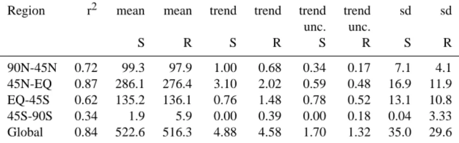
Table 5. Statistical analysis of the synthetic (S) annual emissions, and the retrieved (R) annual emissions (Tg CH4yr−1). The standard
deviation (sd) is a measure of the inter-annual variability. The trend is associated with a calculated uncertainty (trend unc.) using the ± 1 σ interval. Correlation coefficient r2is calculated using annual values of S and R
Region r2 mean mean trend trend trend trend sd sd unc. unc. S R S R S R S R 90N-45N 0.72 99.3 97.9 1.00 0.68 0.34 0.17 7.1 4.1 45N-EQ 0.87 286.1 276.4 3.10 2.02 0.59 0.48 16.9 11.9 EQ-45S 0.62 135.2 136.1 0.76 1.48 0.78 0.52 13.1 10.8 45S-90S 0.34 1.9 5.9 0.00 0.39 0.00 0.18 0.04 3.33 Global 0.84 522.6 516.3 4.88 4.58 1.70 1.32 35.0 29.6
The largest uncertainty pertaining to our method is whether a prescribed zonal field for a single year modified with a trend derived from a limited set of measurements can be used to retrieve trends in emissions and to deduce variabil-ity. To evaluate this difficult problem, we generated a set of synthetic emissions, which consisted of the emission data-set evaluated by Houweling et al. (2000) supplemented with an artificial, but realistic trend of 1% yr−1for all anthropogenic emissions. In addition we applied an artificial variability on the biomass burning and wetland emissions, which are con-sidered to be the main sources of inter-annual variability. We assumed a period of 2 and 4 years and amplitude of 33% and 25%, respectively. The variability of the synthetic emis-sions was on purpose chosen very high to provide a rigorous test for our method. In the next step the monthly and zonal average field for 1987 was calculated, and the surface layer CH4 concentrations at the locations of the 12 NOAA sites
were used to calculate the global 1979–1993 trend. These zonal average concentrations and their trends were then used to ‘nudge’ the model. The further steps followed the same procedure as described before, using varying OH fields and varying meteorology. Shortly, the method tests to what ex-tent the information contained in a limited amount of data can be used to retrieve relatively variable and complex emis-sions. However, the method is not able to test errors in model transport and station representativity on the model’s spatial scale. Figure 8 shows the annual average original synthetic and recalculated emissions. The corresponding statistical pa-rameters are presented in Table 5. Overall, the average emis-sions, the variability and trend are indeed recovered using the method, and high correlation is found between the prescribed and calculated emissions. Except for the southernmost re-gion, the retrieved emissions are within a few percent of the original emissions. Retrieved trends are about 30% lower on the Northern Hemisphere and about 100% higher on the Southern Hemisphere. Globally the errors seem to balance. Except in the 45 S–90 S compartment, the retrieved variabil-ity is 20–30% less than the prescribed ones, due to the use of the ‘background’ station data, and the associated loss of
information.
The largest obvious deviation is found in the region 45 S– 90 S, where spurious emissions are calculated. However, the maximum deviation of the retrieved and synthetic emissions is of similar magnitude (about 10 Tg CH4 yr−1) as in other
regions. Interestingly, the emissions calculated using ‘real’ measurements show much less variability than in this syn-thetic case. We therefore think that the annual trends and 2-D CH4fields are more representative for the ‘real’
situa-tion. Given the rigorous conditions in this test it is therefore quite likely that the trend of CH4 can be retrieved with an
accuracy substantially better than 50%.
References
Aardenne, J. A., Dentener, F. J., Olivier, J. G. J., Klein Goldewijk, C. G. M., and Lelieveld, J.: A 1◦×1◦resolution data set of histor-ical anthropogenic trace gas emissions for the period 1890–1990, Global Biogeochem. Cycles, 15, 909–928, 2001.
Barbosa, P. M., Stroppiana, D., Gregoire, J.-M., and Pereira, J. M. C.: An assessment of vegetation fire in Africa (1981–1991): Burned areas, burned biomass, and atmospheric emission, Global Biogeochem. Cycles, 18, 933–95, 1999.
Bekki, S., Law, K. S., and Pyle, J. A.: Effect of ozone depletion on atmospheric CH4and CO concentrations, Nature, 371, 595–597, 1994.
Br¨uhl, C. and Crutzen, P. J.: MPIC two-dimensional model, NASA Ref. Publ., 1292, 103–104, 1993.
Dentener, F. J. and Crutzen, P. J.: A three-dimensional model of the global ammonia cycle, J. Atmos. Chem., 19, 331–369, 1994. Dentener, F. J., Peters, W., Krol, M., van Weele, M., Bergamaschi,
P., and Lelieveld, J.: On the inter-annual-variability and trend of OH and the lifetime of CH4: 1979–1993 global CTM
simula-tions, J. Geophys. Res., submitted, 2002.
Dlugokencky, E. J., Masarie, K. A., Tans, P. P., Conway, T. J., and Xiong, X.: Is the amplitude of the methane seasonal cycle chang-ing?, Atmos. Environ., 31, 21–26, 1997.
Dlugokencky, E. J., Masarie, K. A., Lang, P. M., and Tans, P. P.: Continuing decline in the growth rate of the atmospheric methane burden, Nature, 393, 447–450, 1998.
Etheridge, D. M., Steele, L. P., Francy, R. J., and Langenfelds, R. L.: Atmospheric methane between 1000 A. D. and present: Evidence of anthropogenic emissions and climatic variability, J. Geophys. Res., 103, 15 979–15 993, 1998.
Fortuin, J. P. F. and Kelder, H.: An ozone climatology based on ozonesonde and satellite measurements, J. Geophys. Res., 103, 31 709–31 734, 1998.
Fung, I., John, J., Lerner, J., Matthews, E., Prather, M., Steele, L. P., and Fraser, P. J.: Three-dimensional model synthesis of the global methane cycle, J. Geophys. Res., 96, 13 033–13 065, 1991.
Ganzeveld, L., Lelieveld, J., and Roelofs, G. J.: A dry deposition parameterization for sulfur oxides in a chemistry and general cir-culation model, J. Geophys. Res., 103, 5679–5694, 1998. Gibson, R., Kallberg, P., and Uppsala, S.: The ECMWF re-analysis
(ERA) project, ECMWF Newsletter 73, European Centre for Medium Range Weather Forecasts, Reading, England, 1997. Guelle, W., Balkanski, Y. J., Schulz, M., Dulac, F., and Monfray,
P.: Wet deposition in a global size-dependent aerosol transport model, Comparison of a 1 year Pb210 simulation with ground measurements, J. Geophys. Res., 103, 11 429–11 445, 1998. Gupta, M., Cicerone, R. J., and Elliot, S.: Perturbation to global
tropospheric oxidizing capacity due to latitudinal redistribution of surface sources of NOx, CH4, and CO, Geophys. Res. Lett.,
21, 3931–3934, 1998.
Heimann, M.: The global atmospheric tracer model TM2, Tech. Rep. 10, Deutsches Klimarechenzentrum, Hamburg, Germany, 1995.
Hein, R., Crutzen, P. J., and Heimann, M.: An inverse modeling approach to investigate the global atmospheric methane cycle, Global Biogeochem. Cycles, 11, 43–76, 1997.
Hogan, K. B. and Harris, R. C.: Comment on “A decrease in the growth rate of atmospheric methane in the Northern Hemisphere during 1992” by E. J. Dlugokencky et al., Geophys. Res. Lett., 21, 2445–2446, 1994.
Houweling, S., Dentener, F. J., and Lelieveld, J.: The impact of non-methane hydrocarbon compounds on tropospheric photochem-istry, J. Geophys. Res., 103, 10 673–10 696, 1998.
Houweling, S., Kaminski, T., Dentener, F. J., Lelieveld, J., and Heimann, M.: Inverse modeling of methane sources and sinks using the adjoint of a global transport model, J. Geophys. Res., 104, 26 137–26 160, 1999.
Houweling, S., Dentener, F. J., Lelieveld, J., Walter, B., and Dlugo-kencky, E. J.: The modeling of tropospheric methane: How well can point measurements be reproduced by a global model?, J. Geophys. Res., 105, 8981–9002, 2000.
Kaminski, T.: Interactive comment on Trends and inter-variability of methane emissions derived from 1979–1993 global CTM sim-ulations by F. Dentener et al., Atmos. Chem. Phys. Discuss., 2, S76–S79, 2002.
Karlsd`ottir, S., Isaksen, I. S. A., G., G. M., and Berntsen, T.: Trend analysis of O3 and CO in the period 1980–1996: A
three-dimensional model study., J. Geophys. Res., 105, 28 907–28 933, 2000.
Krol, M. and Van Weele, M.: Implications of variation of photodis-sociation rates for global atmospheric chemistry, Atmos. Env., 31, 1257–1273, 1997.
Krol, M., van Leeuwen, P. J., and Lelieveld, J.: Global OH trend in-ferred from methylchloroform measurements, J. Geophys. Res.,
103, 10 697–10 711, 1998.
Krol, M., Van Leeuwen, P. J., and Lelieveld, J.: Reply to the com-ment of Prinn and Huang on “Global OH trend inferred from methylchloroform measurements’ by Krol et al., J. Geophys. Res., 106, 23 159–23 164, 2001.
Landgraf, I. and Crutzen, P. J.: An efficient method for online cal-culations of photolysis and heating rates, J. Atmos. Sci., 55, 863– 878, 1998.
Langenfelds, R., Francey, J., Pak, B., Steele, P., Lloyd, J., Trudinger, C., and Allison, C.: The use of multi-species for in-terpreting interannual variability in the carbon cycle, 2001. Lassey, K. R., Lowe, D. C., Brenninkmeijer, C. A. M., and Gomez,
A. J.: Atmospheric methane and its carbon isotopes in the South-ern Hemisphere: Their time series and an instructive model, Chemosphere, 26, 95–109, 1993.
Law, R. and Simmonds, I.: The sensitivity of deduced CO2sources
and sinks to variations in transport and imposed surface concen-trations, Tellus, Ser. B, 48, 613–625, 1996.
Lelieveld, J. and Dentener, F. J.: What controls tropospheric ozone?, J. Geophys. Res., 105, 3531–3551, 2000.
Lelieveld, J., Crutzen, P. J., and Dentener, F. J.: Changing concen-tration, lifetime and climate forcing of atmospheric methane, Tel-lus, Ser. B, 50, 128–150, 1998.
Louis, J. F.: A parametric model of vertical eddy fluxes in the atmo-sphere, Boundary Layer Meteorol., 17, 187–202, 1979. Marland, G., Boden, T. A., and Andres, R. J.: CO2 emissions.
trends: A compendium of data on global change, Tech. rep., Car-bon Dioxide Analysis Center, Oak Ridge National Laboratory, Oak Ridge, Tenn USA, 2000.
McPeters, R.: Nimbus-7 total ozone mapping spectrometer (toms) data products user’s guide, Reference publication 1384, NASA, Washington DC, 1996.
Midgley, P. M. and McCulloch, A.: The production and global dis-tribution of emissions to the atmosphere of 1,1,1-trichloroethane (methyl chloroform), Atmos. Environ., 29, 1601–1608, 1995. Olivier, J. G. J. and Berdowski, J.: Global emissions sources and
sinks, in: The climate system, (Eds) Guicherit, R. and Heij, B. J., A.A. Balkema Publishers/Swets and Zeitlinger Publishers, Lisse, The Netherlands, 2001.
Olivier, J. G. J., Bouwman, A. F., Berdowski, J. J. M., Veldt, C., Bloos, J. P. J., Visschedijk, A. J. H., van der Maas, C. W. M., and Zandveld, P. Y. J.: Sectoral emission inventories of greenhouse gases for 1990 on a per country basis as well as on 1◦×1◦, Environ. Sci. Policy, 2, 241–263, 1999.
Peters, W., Krol, M., Dentener, F. J., and Lelieveld, J.: Identifica-tion of an El Ni˜no oscillaIdentifica-tion signal in a multiyear global sim-ulation of tropospheric ozone, J. Geophys. Res., 106, 19 389– 19 402, 2001.
Prather, M., Ehhalt, D., Dentener, F., Derwent, R., Dlugokencky, E., Holland, E., Isaksen, I., Katima, J., Kirchhoff, V., Matson, P., Midgley, P., and Wang, M.: Atmospheric chemistry and green-house gases, chapter 4, in: Climate Change 2001, The scien-tific basis: Contribution of working group I to the Third assess-ment report of the Intergovernassess-mental Panel on Climate, (Eds) Houghton, J. T., Ding, Y., Griggs, D. J., Noguer, M., van der Lin-den, P. J., Dai, X., Maskell, K., and Johnson, C. A., p. 881, Cam-bridge University Press, CamCam-bridge, United Kingdom and New York, NY, US., 2001.
from methylchloroform measurements” by Krol et al., J. Geo-phys. Res., 106, 23 151–23 157, 2001.
Prinn, R. G., Weiss, R. F., Miller, B. R., Huang, J., Alyea, F. N., Cunnold, D. M., Fraser, P. B., Hartley, D. E., and Simmonds, P. G.: Atmospheric trends and lifetime of CH3CCl3and global
average hydroxyl radical concentrations based on 1978–1994 ALE/GAGE measurements, Science, 269, 187–192, 1995. Prinn, R. G., Huang, J., Weiss, R. F., Cunnold, D. M., Fraser,
P. J., Simmonds, P. G., Mcculloch, A., Harth, C., Salameh, P., O’Doherty, S., Wang, R. J., Porter, L., and Miller, B. R.: Evi-dence for substantial variations of atmospheric hydroxyl radicals in the past two decades, Science, 292, 1882–1888, 2001. Rayner, P.: Interactive comment on Trends and inter-variability of
methane emissions derived from 1979–1993 global CTM simu-lations by F. Dentener et al., Atmos. Chem. Phys. Discuss., 2, S158–S163, 2002.
Russell, G. and Lerner, J.: A new finite-differencing scheme for the tracer transport equation, J. Appl. Meteorol., 20, 1483–1498, 1981.
Sander, S. P., Friedl, R. R., DeMore, W. B., Kurylo, M. J., Hamp-son, R. F., Huie, R. E., Moortgat, G. K., Ravishankara, A. R., Hampson, C. E. K., J., C., and Molina, M. J.: Chemical kinet-ics and photochemical data for use in stratospheric modelling, NASA/JPL publ. 00-003 Eval. 13, Jet Propul. Lab., Pasadena, California, USA, 2000.
Tiedke, M.: A comprehensive mass flux scheme for cumulus pa-rameterization in large-scale models, Mon. Weather Rev., 117, 1779–1800, 1989.
Walter, B. P., Heimann, M., and Matthews, E.: Modeling modern methane emissions from natural wetlands 2., interannual varia-tions 1982–1993, J. Geophys. Res., D24, 34 207–34 129, 2001. Wild, O. and Prather, M.: Excitation of the primary tropospheric
chemical mode in a global three-dimensional model, J. Geophys. Res., 105, 24 647–24 660, 2000.
Ziemke, J., Chandra, S., and Bartia, P.: Seasonal and interannual variabilities in tropical tropospheric ozone, J. Geophys. Res., 104, 21 245–21 442, 1999.
![Fig. 3. Methane lifetime [years] determined for 3 simulations, for the 4 regions and global.](https://thumb-eu.123doks.com/thumbv2/123doknet/14544186.535945/8.892.126.765.90.613/fig-methane-lifetime-years-determined-simulations-regions-global.webp)