HAL Id: hal-03142102
https://hal.uca.fr/hal-03142102
Submitted on 15 Feb 2021
HAL is a multi-disciplinary open access
archive for the deposit and dissemination of
sci-entific research documents, whether they are
pub-lished or not. The documents may come from
L’archive ouverte pluridisciplinaire HAL, est
destinée au dépôt et à la diffusion de documents
scientifiques de niveau recherche, publiés ou non,
émanant des établissements d’enseignement et de
On some graph classes related to perfect graphs: A
survey
Flavia Bonomo-Braberman, Guillermo Durán, Martín Safe, Annegret Wagler
To cite this version:
Flavia Bonomo-Braberman, Guillermo Durán, Martín Safe, Annegret Wagler. On some graph classes
related to perfect graphs: A survey. Discrete Applied Mathematics, Elsevier, 2020, 281, pp.42-60.
�10.1016/j.dam.2019.05.019�. �hal-03142102�
On graph classes related to perfect graphs:
A survey
Flavia Bonomo
1, Guillermo Dur´
an
2, Mart´ın D. Safe
3, and
Annegret K. Wagler
4 1Universidad de Buenos Aires. Facultad de Ciencias Exactas y
Naturales. Departamento de Computaci´on. /
CONICET-Universidad de Buenos Aires. Instituto de
Investigaci´on en Ciencias de la Computaci´on (ICC). Buenos
Aires, Argentina, [email protected]
2Universidad de Buenos Aires. Facultad de Ciencias Exactas y
Naturales. Departamento de Matem´atica. /
CONICET-Universidad de Buenos Aires. Instituto de C´alculo
(IC). Buenos Aires, Argentina / Departamento de Ingenier´ıa
Industrial, Facultad de Ciencias F´ısicas y Matem´aticas,
Universidad de Chile, Santiago, Chile, [email protected]
3Departamento de Matem´atica, Universidad Nacional del Sur,
Bah´ıa Blanca, Argentina / INMABB (UNS-CONICET), Bah´ıa
Blanca, Argentina, [email protected]
4Laboratoire d’Informatique, de Mod´elisation et d’Optimisation des
Syst`emes (LIMOS, UMR CNRS 6158), Universit´e Clermont
Auvergne, Clermont-Ferrand, France, [email protected]
Abstract
Perfect graphs form a well-known class of graphs introduced by Berge in the 1960s in terms of a min-max type equality involving two famous graph parameters. In this work, we study variants and subclasses of per-fect graphs defined by means of min-max relations of other graph pa-rameters. Our focus is on clique-perfect, coordinated, and neighborhood-perfect graphs. We show the connection between graph classes and both hypergraph theory and the clique graph operator. We review different par-tial characterizations of them by forbidden induced subgraphs, present the previous results, and the main open problems. Computational complexity problems are also discussed.
1
Introduction
Perfect graphs were defined by Berge in the 1960s in terms of a min-max type equality involving two important parameters: the clique-number and the
chro-matic number. Coloring a graph is the task of assigning colors to its vertices
in such a way that no two adjacent vertices receive the same color. In many situations we are interested in knowing the minimum number of different colors needed to color a certain graph G. This minimum number is called the
chro-matic number of G and is denoted by χ(G). A complete is a set of vertices
that are pairwise adjacent and a clique is a complete set that is not properly contained in any other. The maximum cardinality of a clique of a graph G is called the clique number of G and is denoted by ω(G). Clearly, in any coloring, the vertices of a clique must receive different colors. Thus, ω(G) is a trivial lower bound for χ(G), i.e., the min-max type inequality
ω(G) ≤ χ(G) holds for any graph G.
Moreover, the difference between χ(G) and ω(G) can be arbitrarily large. My-cielski presented in [61] a family of graphs {Gn}n≥2 with ω(Gn) = 2 and
χ(Gn) = n. In this context, Berge defined a graph G to be perfect if and only if
the min-max type equality ω(G′) = χ(G′) holds for each induced subgraph G′
of G.
Min-max type relations play a remarkable role in the field of discrete mathe-matics. In the following pages, we will recall two famous min-max type theorems due to K˝onig for bipartite graphs. Other notable examples are Dilworth’s theo-rem [31] that dictates that in any partial order the maximum size of an antichain equals the minimum number of chains needed to cover it, Menger’s theorem [60] that states that the maximum number of disjoint paths joining two vertices s and t equals the minimum number of edges in an st-cut, and its generalization, the max-flow min-cut theorem [40] that ensures that the maximum amount of flow in a network equals the capacity of a minimum cut.
The complement of a graph G is the graph G whose vertex set is the same as the vertex set of G but such that any pair of different vertices are adjacent in G if and only if they are nonadjacent in G. In 1972, Lov´asz, and shortly after Fulkerson, proved a conjecture by Berge stating the following:
Theorem 1 (Perfect Graph Theorem [56]) A graph is perfect if and only
if its complement is perfect.
A stable set of a graph is a set of vertices that are pairwise nonadjacent. The
stability number of a graph G is the maximum cardinality α(G) of a stable set of
G. The clique covering number of a graph G is defined as the minimum number of cliques of G needed to cover the vertices of G, and it is denoted by θ(G). Clearly, α(G) ≤ θ(G). Moreover, α(G) = ω(G) and θ(G) = χ(G). Therefore, by the Perfect Graph Theorem, the notion of perfection can also be formulated in terms of a min-max type equality involving the stability number and the
clique covering number: a graph G is perfect if and only if α(G′) = θ(G′) for
each induced subgraph G′ of G.
A hole is a chordless cycle of length at least 5 (a chord is an edge joining two nonconsecutive vertices of the cycle). An antihole is the complement of a hole. A hole, or antihole, is said odd or even if it has an odd or an even number of vertices. We say that a graph has an odd hole (resp. antihole) if it contains an induced odd hole (resp. antihole). A hole of length n is denoted by Cn.
It is not difficult to verify that odd holes and odd antiholes are imperfect (i.e., not perfect). Since the class of perfect graphs is hereditary, any perfect graph has no odd holes and no odd antiholes. Furthermore, Berge conjectured, and Chudnovsky, Robertson, Seymour, and Thomas proved the following forbidden
induced subgraph characterization for perfect graphs:
Theorem 2 (Strong Perfect Graph Theorem (SPGT) [24]) A graph G
is perfect if and only if G has no odd hole and no odd antihole.
Shortly before, Chudnovsky, Cornu´ejols, Liu, Seymour, and Vuˇskovi´c devised a polynomial-time algorithm for recognizing perfect graphs [23].
The class of clique-perfect graphs is defined in a somewhat similar fashion. A
clique-independent set of a graph G is a subset of pairwise disjoint cliques of G.
A clique-transversal of G is a subset of vertices intersecting all the cliques of G. Denote by αc(G) and τc(G) the maximum cardinality of a clique-independent set
and the minimum cardinality of a clique-transversal of G, respectively. Clearly, the min-max type inequality
αc(G) ≤ τc(G) holds for any graph G.
In analogy to perfect graphs, a graph G is said to be clique-perfect if and only if αc(G′) = τc(G′) holds for each induced subgraph G′ of G. A graph that
is not clique-perfect is said clique-imperfect. It is important to mention that clique-perfect graphs do not need to be perfect since, for instance, odd antiholes of length 6n + 3 are clique-perfect for each n ≥ 1 (Reed, 2001, cf. [36]). The difference between αc(G) and τc(G) can be arbitrarily large. Dur´an, Lin, and
Szwarcfiter presented in [36] a family of graphs {Gn}n≥2such that αc(Gn) = 1
and τc(Gn) = n where the number of vertices of Gn grows exponentially. Later,
Lakshmanan S. and Vijayakumar [51] found another family of graphs {Hn}n≥1
such that αc(Hn) = 2n + 1 and τc(Hn) = 3n + 1 but Hnhas only 5n + 2 vertices.
The equality between αc(G) and τc(G) has been implicitly studied in the
lit-erature for long time, but the name ‘clique-perfect’ was first introduced by Gu-ruswami and Pandu Rangan [47]. Some well-known graph classes being clique-perfect are: balanced graphs [7], comparability graphs [2], dually chordal graphs [19], complements of acyclic graphs [9], and distance-hereditary graphs [52].
A matching of a graph G is a set of edges that pairwise do not share end-points. A vertex cover of G is a set S of vertices of G such that every edge of G has at least one endpoint in S. The matching number ν(G) is the maximum cardinality of a matching of G, and the vertex covering number τ (G) is the
minimum cardinality of a vertex cover. K˝onig’s matching theorem [49] asserts that the min-max equality
ν(G) = τ (G) holds for any bipartite graph G.
Notice that if G is bipartite and with no isolated vertices then the cliques of G coincide with its edges and, as a consequence, αc(G) = ν(G) and τc(G) = τ (G).
Then, by K˝onig’s matching theorem, if G is bipartite and without isolated vertices then αc(G) = τc(G). It is easily seen that this equality holds even if
the bipartite graph G is permitted to have isolated vertices. Since the induced subgraphs of a bipartite graph are also bipartite then bipartite graphs are perfect. Thus, bipartite graphs can be regarded as a special type of clique-perfect graphs.
Coordinated graphs form a subclass of perfect graphs and are defined
simi-larly. Let G be a graph, let γc(G) be the minimum number of colors needed to
color the cliques of G in such a way that two intersecting cliques receive different colors, and let ∆c(G) be the maximum cardinality of a family of cliques all of
which have at least one vertex of G in common. Clearly, ∆c(G) ≤ γc(G) holds for any graph G.
Parameters ∆c and γc are generally denoted in the literature by M and F ,
respectively.
A graph G is called coordinated if ∆c(G′) = γc(G′) for each induced subgraph
G′ of G. Since the class of coordinated graphs is hereditary by definition, and
since odd holes and odd antiholes are not coordinated [12] then, by the SPGT, coordinated graphs are perfect. Also in this case, the difference between the parameters can be arbitrarily large. In fact, in [12] it is shown that, for antiholes, the difference γc(Cn) − ∆c(Cn) grows exponentially in n.
If G is a triangle-free graph without isolated vertices, the cliques of G coincide with the edges, then γc(G) coincides with γ(G), the so called chromatic index
(minimum number of colors to color the edges of a graph so that edges that share an endpoint receive different colors), and the parameter ∆c(G) coincides
with the maximum degree ∆(G) of the vertices of G. By K˝onig’s edge coloring theorem [49],
γ(G) = ∆(G) holds for any bipartite graph G.
As in the case of clique-perfection, we can conclude that γc(G) = ∆c(G) holds
for any bipartite graph G and hence bipartite graphs are coordinated. Thus, coordinated graphs constitute another way of generalizing bipartite graphs.
Neighborhood-perfect graphs were defined in [53], also by the equality of two
parameters for all induced subgraphs. Given a graph G, a set C ⊆ V (G) is a
neighborhood-covering set (or neighborhood set) if each edge and each vertex of G
belongs to G[v] for some v ∈ C, where G[v] denotes the subgraph of G induced by the closed neighborhood of the vertex v. Two elements of E(G) ∪ V (G) are neighborhood-independent if there is no vertex v ∈ V (G) such that both
Figure 1: Some small graphs
elements are in G[v]. A set S ⊆ V (G) ∪ E(G) is said to be a
neighborhood-independent set if every pair of elements of S is neighborhood-neighborhood-independent.
Let ρn be the size of a minimum neighborhood-covering set and αn(G) of a
maximum neighborhood-independent set. Clearly, ρn≥ αn(G) for every graph
G. When ρn(G′) = αn(G′) for every induced subgraph G′ of G, G is called
a neighborhood-perfect graph. It was proved in [53] that odd holes and odd antiholes are not neighborhood-perfect and hence, the Strong Perfect Graph Theorem implies that neighborhood-perfect graphs are also perfect.
In Section 2 we present the basic definitions and preliminary results. In Sec-tion 3 we discuss the connecSec-tion between our subject and hypergraph theory. In Section 4 we study how clique-perfection and coordination depend on prop-erties of the clique graph. In Section 5 the studied variants of perfect graphs are analyzed when restricted to different graph classes, detailing the previous results and providing some new contributions and open problems.
2
Definitions and preliminaries
All graphs in this paper are undirected, without loops and without multiple edges. We denote the vertex set of the graph G by V (G), and the edge set by E(G). For any set S, |S| will denote its cardinality. Cn will denote the
chordless cycle with n vertices, Pnthe chordless path with n vertices, and Kn a
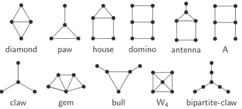
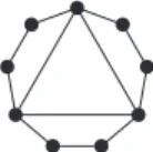
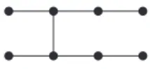
complete with n vertices. Path and cycles are assumed to be simple (i.e., with no repeated vertices aside from the starting and ending vertices in the case of cycles). A cycle of a graph is Hamiltonian if it visits every vertex of the graph. By the edges of a cycle we mean those edges joining two consecutive vertices of the cycle. A triangle is a complete with three vertices. A graph is triangle-free if it contains no induced triangle. Some small graphs to be referred in the sequel are depicted in Figure 1.
A universal vertex in a graph is a vertex that is adjacent to all the other vertices of the graph. An isolated vertex is a vertex that is not adjacent to any other vertex of the graph. The neighborhood of a vertex v in a graph G is the set NG(v) consisting of all the vertices that are adjacent to v. The degree of v
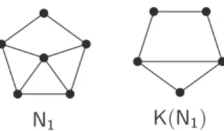
Figure 2: The graph N1 and its clique graph
is dG(v) = |NG(v)|. The common neighborhood of an edge e = vw is NG(e) =
NG(v)∩NG(w), and, in general, the common neighborhood of a nonempty subset
W of vertices is NG(W ) =
T
w∈WNG(w), while NG(∅) = V (G). If H is a
subgraph of G then NH(v) = NG(v) ∩ V (H), NH(e) = NG(e) ∩ V (H) and
NH(W ) = NG(W ) ∩ V (H) for every vertex v, every edge e and every subset
of vertices W . The closed neighborhood of v is the set NG[v] = NG(v) ∪ {v}.
Two vertices v and w are true twins in G if NG[v] = NG[w], and false twins if
NG(v) = NG(w). The subgraph of G induced by the vertex set W ⊆ V (G) is
denoted by G[W ], and G − W denotes G[V (G) \ W ]. A vertex set W ⊆ V (G) is a vertex covering of G if each edge of G has at least one endpoint in W .
A graph G is anticonnected if G is connected. An anticomponent of G is the subgraph of G induced by the vertices of a connected component of G.
A class C of graphs is called hereditary if, for every graph of C, all its induced subgraphs belong to C. Let G and H be graphs. We say that G is H-free to mean that G contains no induced H. If H is a collection of graphs we say that G is H-free to mean that G contains no induced H for any H ∈ H.
Let F be a family of sets. The intersection graph of F is a graph whose vertices are the members of F, and such that two members of F are adjacent if and only if they intersect. For instance, the line graph L(G) of a graph G is the intersection graph of the edges of G. Whitney [76] proved that if H and H′
are connected graphs such that L(H) = L(H′) 6= K
3 then H = H′.
Another example of an intersection graph is the clique graph. The clique
graph K(G) of a graph G is the intersection graph of the cliques of G. The
map K : G 7→ K(G) is known as the clique graph operator or simply the clique
operator. A graph G is said to be perfect if K(G) is perfect. If G is not
K-perfect we say that it is K-imK-perfect. Notice that the class of K-K-perfect graphs is not hereditary. For instance, the graph N1 of Figure 2 is K-perfect but it
contains an induced C5 and K(C5) = C5 is imperfect. Because of this, the
following terminology is introduced in [66]: a graph is hereditary K-perfect if all its induced subgraphs are K-perfect. It turns out that hereditary K-perfect graphs are perfect, as implied by the SPGT together with the following lemma. Lemma 3 ([66]) A hereditary K-perfect graph has no odd holes and has no
antiholes with more than 6 vertices.
Proof. It is clear that hereditary K-perfect graphs have no odd holes since odd
holes are K-imperfect. All along the proof, Cn will denote the graph such that
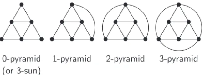
Figure 3: From left to right: 0-, 1-, 2- and 3-pyramid
n ≥ 5 and n 6= 6, 7, 9, 12. By elementary number theory, n = 5a + 3b for some a ≥ 1 and some b ≥ 0. This implies that there exists a sequence a1, . . . , ak
of integers taken from the set {2, 3} that satisfies the following conditions: (i ) a1+ · · · + ak = n; (ii ) ai = 2 for some i ∈ {1, . . . , k}; and (iii ) for each
j = 1, . . . , k, aj = 2 implies aj+1 = 3 (where ak+1 means a1). Assume such a
sequence {ai} is given and define bi equal to a1+ · · · + ai modulo n for each
i = 1, . . . , k. In particular, bk = 0. Let Q1 = {b1, b2, . . . , bk}, Q2 = Q1+ 2,
Q3 = Q1+ 4, Q4= Q1+ 1, and Q5 = Q1+ 3, where A + p = {a + p : a ∈ A}
and the sum is taken modulo n. Then, Qi is a clique of Cn for i = 1, 2, . . . , 5
and, by construction, Q1Q2. . . Q5 is an odd hole in K(Cn). Finally, observe
that K(C7) = C7; that if Q1= {0, 2, 4, 6} then {Q1, Q1+ 1, Q1+ 2, . . . , Q1+ 8}
induces a C9 in K(C9); and that if Q1 = {0, 2, 5, 7, 9} and Q2= {1, 3, 5, 7, 10}
then {Q1, Q1+ 1, Q1+ 2, Q1+ 3, Q1+ 9, Q2, Q2+ 1, Q2+ 2, Q2+ 3} induces a
C9 in K(C12). ¤
Interestingly, hereditary K-perfection has been implicitly characterized when restricted to several graph classes; many of these characterizations are presented in Section 5.
A family F of nonempty sets is said to satisfy the Helly property if every nonempty subfamily of F of pairwise intersecting members has nonempty in-tersection. A graph G is said to be clique-Helly (CH) if the family of its cliques satisfies the Helly property. The graphs of Figure 3 are examples of graphs that are not clique-Helly. Clique-Helly graphs were characterized in [32] and inde-pendently in [71]. Notice that any graph with a universal vertex is clique-Helly and thus a clique-Helly graph may contain any prescribed induced subgraph. Instead, a graph is hereditary clique-Helly (HCH) [64] if all its induced sub-graphs are clique-Helly. Prisner gave several characterizations of hereditary clique-Helly graphs, one by means of minimal forbidden induced subgraphs: Theorem 4 ([64]) A graph is hereditary clique-Helly if and only if it contains
none of the graphs of Figure 3 as induced subgraph.
In the sequel, we call any of the graphs in Figure 3 a pyramid. The graph 0-pyramid is also called 3-sun. In [64] and [74], it is proved that a hereditary clique-Helly graph G has at most |V (G)| + |E(G)| cliques.
union of G and H is a graph G ∪ H whose vertex set is V (G) ∪ V (H) and
whose edge set is E(G) ∪ E(H). The disjoint union is clearly an associative operation, and for each nonnegative integer t we will denote by tG the disjoint union of t copies of G. The join of G and H is a graph G+H whose vertex set is V (G)∪V (H) and whose edge set is E(G)∪E(H)∪{vw : v ∈ V (G), w ∈ V (H)}. A graph is bipartite if its vertex set can be partitioned into two (possibly empty) stable sets. A graph is chordal if every cycle of length at least 4 has at least one chord. A comparability graph is a graph that admits a transitive acyclic orientation of its edges. Bipartite and chordal graphs can be recognized in linear time and comparability graphs can be recognized in polynomial time [65, 70]. Bipartite, chordal and comparability graphs are subclasses of perfect graphs.
A cograph [29] is a P4-free graph, that is, a graph without chordless paths on
4 vertices. Equivalently, cographs are those graphs that can be obtained from isolated vertices by successively applying disjoint union and join operations. Cographs form a well-known class of perfect graphs.
We will study in this survey two superclasses of cographs: P4-tidy graphs
and tree-cographs. A graph G = (V, E) is P4-tidy if for every vertex set A
inducing a P4 in G there is at most one vertex v ∈ V \ A such that G[A ∪ {v}]
contains at least two induced P4’s. They were introduced in [45]. A starfish is
a graph whose vertex set can be partitioned into three sets S, C and R, where each of the following conditions holds: (1) S = {s1, . . . , st} is a stable set and
C = {c1, . . . , ct} is a clique, for some t ≥ 2; (2) siis adjacent to cj if and only if
i = j; and (3) R is allowed to be empty and if it is not, then all the vertices in R are adjacent to all the vertices in C and nonadjacent to all the vertices in S. An urchin is a graph whose vertex set can be partitioned into three sets S, C, and R satisfying the same conditions (1) and (3) but that instead of condition (2) satisfies: (2’) siis adjacent to cjif and only if i = j. Clearly, urchins are the
complements of starfishes and vice versa. A fat starfish (resp. fat urchin) arises from a starfish (resp. urchin) with partition (S, C, R) by substituting exactly one vertex of S ∪ C by K2 or 2K1.
Theorem 5 ([45]) If G is a P4-tidy graph, then exactly one of the following
statements holds:
1. G or G is disconnected;
2. G is isomorphic to C5, P5, P5, a starfish, a fat starfish, an urchin, or a
fat urchin.
Tree-cographs were defined in [72] by the following recursive definition: 1. Every tree is a tree-cograph.
2. If G is a tree-cograph, then G is a tree-cograph. 3. The disjoint union of tree-cographs is a tree-cograph.
This definition implies that if G is a tree-cograph, then either G or G is dis-connected, or G is a tree or the complement of a tree. Tree-cographs are also a subclass of perfect graphs.
Distance-hereditary graphs form another superclass of cographs. A graph G
is called distance-hereditary if and only if the distance between any two vertices of G is the same in every connected induced subgraph of G containing the two vertices. Equivalently, a graph is distance-hereditary if and only if it is {house,domino,gem}-free and has no holes of length at least 5 [3].
A circular-arc graph [46] is the intersection graph of arcs of the unit circle. A representation of a circular-arc graph is a collection of arcs (of the unit circle), each corresponding to a unique vertex of the graph, such that two arcs intersect if and only if the corresponding vertices are adjacent. A Helly circular-arc
(HCA) graph [44] is a circular-arc graph admitting a representation whose arcs
satisfy the Helly property.
Let G be a graph, Q1, . . . , Qk all its cliques and v1, . . . , vn all its vertices.
A clique matrix (or clique-vertex incidence matrix ) of G is the k × n matrix A = (aij) where aij is 1 if vj ∈ Qi and 0 otherwise. The clique matrix of a
graph is unique up to permutations of rows and/or columns. Let A be a m × n zero-one matrix. We say that A is perfect if the set packing polytope
{x ∈ Rn| x ≥ 0, Ax ≤ 1}
has all integer extreme points. Perfect graphs and perfect matrices are related by the following result [26, 63]: a graph is perfect if and only if its clique matrix
is perfect.
A zero-one matrix A is said to be balanced if and only if it contains no odd square submatrix with exactly two 1’s in each row and in each column. Clearly, balancedness is preserved by row permutations, column permutations and transpositions. There is a forbidden submatrix characterization for balanced matrices in terms of perfect matrices: Let A be a zero-one matrix. Then A is
balanced if and only if all submatrices of A are perfect [4, 63]. In particular,
balanced matrices are perfect. By analogy with the relation between perfect graphs and perfect matrices, Dahlhaus, Manuel and Miller proposed to call a graph balanced if its clique matrix is balanced [30]. There is a characterization of balanced graphs in terms of forbidden structures defined as follows. An
unbalanced cycle of a graph G is an odd cycle C such that for each edge e of C
there exists a (possibly empty) complete We of G such that We ⊆ NG(e) \ C
and NC(We) ∩ NC(e) = ∅.
Theorem 6 ([4, 14]) A graph is balanced if and only if it contains no
unbal-anced cycle.
In [64], Prisner proved that a graph is hereditary clique-Helly if and only if its clique matrix does not contain a 3×3 submatrix with exactly two 1’s in each row and in each column. In particular, it turns out that balanced graphs are heredi-tary clique-Helly, thus the number of cliques of a balanced graph is bounded by its number of vertices plus its number of edges. Dahlhaus, Manuel and Miller observed that combining the polynomial-time algorithm in [73] that outputs the clique matrix of a hereditary clique-Helly graph, together with the polynomial-time algorithm in [27] that recognizes balanced matrices, a polynomial-polynomial-time
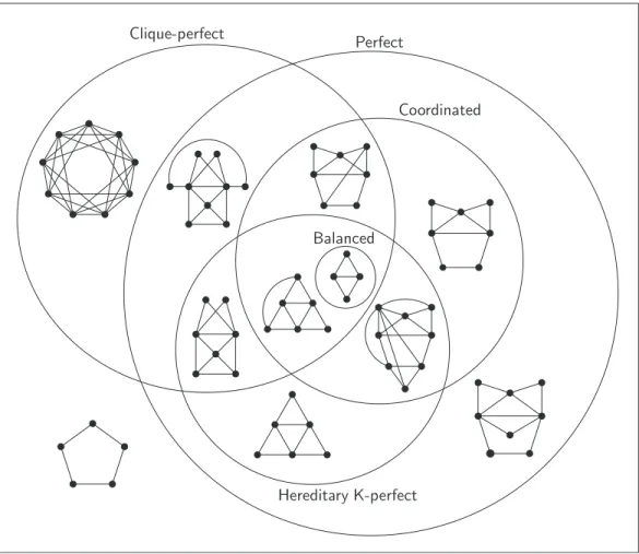
Figure 4: Inclusions and intersections of the studied classes related to coordi-nated graphs, together with separating examples
algorithm to recognize balanced graphs is obtained. The algorithm proposed in [27] by Conforti, Cornu´ejols, Kapoor and Vuˇskovi´c was quite involved, but Zam-belli [77] developed a simpler polynomial-time algorithm to test balancedness of a matrix.
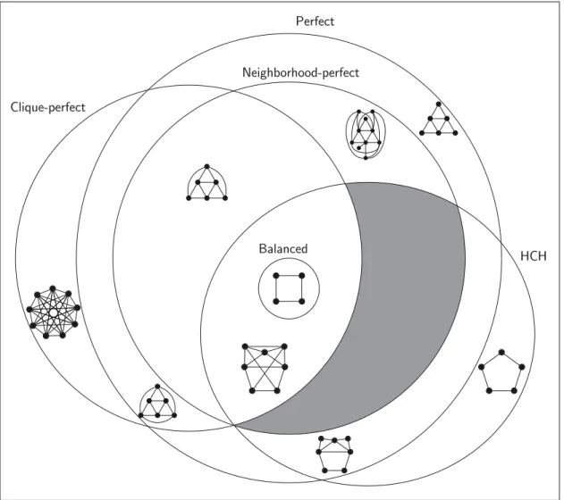
Figures 4 and 5 show the inclusion and intersection schemes of the graph classes that are the subject of this paper related to coordinated and neighborhood-perfect graphs, respectively.
Figure 5: Inclusions and intersections of the studied classes related to neighborhood-perfect graphs, with separating examples. The shaded region corresponds to an empty set.
3
Connection with hypergraph theory
A hypergraph H is an ordered pair (X, E) where X is a finite set and E is a family of nonempty subsets of X. The elements of X are the vertices of H and the elements of E are the hyperedges of H. If x1, . . . , xn are the vertices of
H and E1, . . . , Em are the hyperedges of H then a hyperedge-vertex incidence
matrix of H is the m × n matrix A = (aij) where aij is 1 if xj ∈ Ei and
0 otherwise. A hypergraph has the Helly property if every nonempty family of pairwise intersecting hyperedges has a nonempty intersection. The line graph (or
representative graph) of a hypergraph H, denoted by L(H), is the intersection
graph of the family E of hyperedges of H.
We will restrict ourselves to hypergraphs (X, E) whereSE = X. A partial
hypergraph of H is a hypergraph H′ whose hyperedge set E′ is a subset of the
hyperedge set of H and whose vertex set is the union of the members of E′.
We will be mostly interested in studying clique hypergraphs of graphs. Namely, the clique hypergraph of a graph G is the hypergraph K(G) = (X, E) where X is the set of vertices of G and E is the family of cliques of G. The hyperedge-vertex incidence matrix of K(G) is the clique matrix of G, and G is clique-Helly if and only if K(G) has the Helly property. Besides, clique graph and clique hypergraph are related in the following way: K(G) = L(K(G)).
3.1
The K˝
onig property
A matching of H is a family of pairwise disjoint hyperedges and the matching
number ν(H) is the maximum cardinality of a matching of H. A transversal of
H is a set of vertices that meet all the hyperedges and the transversal number τ (H) is the minimum cardinality of a transversal of H. Clearly, ν(H) ≤ τ (H) for each hypergraph H. A hypergraph is said to satisfy the K˝onig property if
ν(H) = τ (H). Notice that αc(G) = ν(K(G)) and τc(G) = τ (K(G)). Thus, we
have by definition:
Remark 1 A graph G is clique-perfect if and only if the clique hypergraph K(G′)
has the K˝onig property for each induced subgraph G′ of G.
3.2
The colored edge property
Another property of hypergraphs being of our interest is the following. Let H be a hypergraph. The chromatic index γ(H) of H is the least number of colors necessary to color the hyperedges of H such that any two intersecting hyperedges are colored with different colors. The degree dH(x) of a vertex x
of H is the number of hyperedges of H containing x. The maximum degree of the hypergraph H is defined as ∆(H) = maxx∈XdH(x). Clearly, ∆(H) ≤
γ(H) for any hypergraph H. Finally, a graph is said to have the colored edge
property [6, p. 15] if and only if γ(H) = ∆(H). Since γc(G) = γ(K(G)) and
Remark 2 A graph G is coordinated if and only if the clique hypergraph K(G′)
has the colored edge property for each induced subgraph G′ of G.
3.3
Normality
Lov´asz proved the following (we use the formulation of Berge [6, pp. 195–197]): Theorem 7 ([56]) Let H be a hypergraph, AH be the hyperedge-vertex
inci-dence matrix of H and AT
H be its transpose. Then the following conditions are
equivalent:
1. Every partial hypergraph of H has the K˝onig property. 2. Every partial hypergraph of H has the colored edge property. 3. The matrix AT
H is perfect.
4. H satisfies the Helly property and L(H) is perfect.
Any hypergraph satisfying any of these conditions is said to be normal. Since K(G) = L(K(G)), it follows as a corollary:
Corollary 8 Let G be a graph, AG the clique matrix of G and ATG be its
trans-pose. Then the following are equivalent:
1. Every partial hypergraph of K(G) has the K˝onig property. 2. Every partial hypergraph of K(G) has the colored edge property. 3. The matrix AT
G is perfect.
4. G is clique-Helly and K(G) is perfect.
In light of this theorem we introduce the following terminology: a graph G will be called clique-normal if G is clique-Helly and K(G) is perfect, or equivalently, if its clique hypergraph K(G) is normal. Notice that an induced subgraph of a clique-normal graph may not be clique-normal. For instance, the graph N1 of Figure 2 is clique-normal but contains an induced C5 which is not
even K-perfect.
So we introduce also the following definition: a graph G is said to be
hered-itary clique-normal if all the induced subgraphs of G are clique-normal.
Equiv-alently, G is hereditary clique-normal if it is hereditary clique-Helly and hered-itary K-perfect. Combining Corollary 8 with Remarks 1 and 2 it follows: Corollary 9 If G is hereditary clique-normal (i.e., hereditary clique-Helly and
hereditary K-perfect) then G is clique-perfect and coordinated.
The converse is not true because there are graphs that are clique-perfect and coordinated but not even hereditary K-perfect (see Figure 4). Neverthe-less, Corollaries 16 and 20 of Section 4 can be regarded as partial converses of Corollary 9.
A different characterization of clique-normal graphs arises from defining clique subgraphs, which are closer to partial hypergraphs of the clique hyper-graph than induced subhyper-graphs. Let G be a hyper-graph, Q the set of cliques of G and
Q′⊆ Q. Denote by G
Q′ the subgraph of G formed exactly by the vertices and
edges corresponding to the cliques in Q′. If every clique of G
Q′ is also a clique
of G then GQ′ is called a clique subgraph of G [13]. A graph G is called c–clique-perfect if τc(H) = αc(H) for every clique subgraph H of G, and c–coordinated
if γc(H) = ∆c(H) for every clique subgraph H of G.
By definition, if H is a clique subgraph of a graph G then K(H) is an induced subgraph of K(G). This property allows to prove the following theorem: Theorem 10 ([12, 13]) Let G be a clique-normal graph. Then G is
c–clique-perfect and c–coordinated.
Moreover, when G is hereditary clique-Helly, every induced subgraph of K(G) is the clique graph of a clique subgraph of G [64]. So the following holds: Theorem 11 ([12, 13]) Let G be a hereditary clique-Helly graph. Then the
following statements are equivalent: 1. K(G) is perfect.
2. G is c–clique-perfect. 3. G is c–coordinated. 4. G is clique-normal.
It remains an open question whether the equivalence among assertions (1), (2), and (3) of the above theorem holds for (general) clique-Helly graphs G.
Berge defined in 1969 a hypergraph to be balanced (cf. [33, p. 397]) if its hyperedge-vertex incidence matrix is balanced. Recall that balanced graphs are those whose clique matrix is balanced, that is, those graphs whose clique hypergraph is balanced. We have also the following:
Theorem 12 ([7, 56]) If a hypergraph is balanced then it is also normal. Since the class of balanced graphs is hereditary [14, 46] then:
Corollary 13 Balanced graphs are hereditary clique-normal (i.e., hereditary
Helly and hereditary K-perfect). In particular, balanced graphs are clique-perfect and coordinated.
The class of balanced graphs is a common subclass of clique-perfect and coordinated graphs that is interesting from a computational point of view. In fact, the problems of determining each of the parameters αc, τc, ∆c and γc
are NP-complete [20], NP-hard [38], #P-complete [8] and {#P,NP}-hard [8], respectively. However, all these problems are known to be polynomially solvable when restricted to balanced graphs. Indeed, as we already mentioned, the size of the clique matrix of a balanced graph is bounded by a polynomial in the number of vertices and, consequently, can be computed in polynomial time. This, combined with the fact that the set packing and set covering polyhedra of balanced matrices are integral [41], implies the following:
Theorem 14 ([30, 41]) Each of the parameters αc, τc, ∆cand γc can be
Figure 6: An example of an α(K)-perfect and χ(K)-perfect but K-imperfect graph
4
Connection with the clique graph operator
The following result relates the parameters used to define clique-perfect graphs with the parameters used to define perfect graphs applied to the clique graph: Theorem 15 ([13]) Let G be a graph. Then:1. αc(G) = α(K(G)).
2. τc(G) ≥ θ(K(G)).
3. If G is clique-Helly then τc(G) = θ(K(G)).
The theorem above asserts, in particular, that
αc(G) = α(K(G)) ≤ θ(K(G)) ≤ τc(G) holds for any graph G (∗)
and we shall notice that a graph is clique-perfect exactly when both inequalities are satisfied at equality for each of its induced subgraphs.
A graph G is called α-good when α(G) = θ(G), and α-bad otherwise. Con-trary to the case of perfect graphs, the equality is not imposed to the induced subgraphs, and α-goodness is strictly weaker than perfection. We will say that a graph G is α(K)-good if K(G) is α-good, i.e. if α(K(G)) = θ(K(G)). We will say that it is α(K)-bad otherwise. Finally, we define a graph to be α(K)-perfect if each of its induced subgraphs is α(K)-good, or equivalently, if α(K(G′)) = θ(K(G′)) for each induced subgraph G′ of G. The graph
de-picted in Figure 6 is an example of an α(K)-perfect graph that is not hereditary K-perfect. Notice that given a graph G, the clique graph K(G) may contain some induced subgraphs which are not clique graphs of any induced subgraph of G and this is one reason why α(K)-perfection turns out to be strictly weaker property than hereditary K-perfection.
With all this terminology, Theorem 15 implies the following variant of Corol-lary 9:
Corollary 16 ([13]) If G is a clique-perfect graph then G is α(K)-perfect.
Fur-thermore, if G is hereditary clique-Helly then the converse also holds.
Thus the class of α(K)-perfect graphs is a superclass of both clique-perfect graphs and hereditary K-perfect graphs. Below we introduce some graphs that are known to be clique-imperfect and study whether they are α(K)-good or not.
An r-sun or simply sun [39] is a chordal graph G on 2r vertices, r ≥ 3, whose vertex set can be partitioned into two sets, W = {w1, . . . , wr} and U =
{u1, . . . , ur}, such that W is a stable set and for each i and j, wj is adjacent to
ui if and only if i = j or i ≡ j + 1 mod r. A sun is odd if r is odd. A sun is
complete if U is a complete.
The concept of suns was later extended as follows. Let G be a graph and C be a cycle of G not necessarily induced. An edge of C is non-proper (or
improper ) if it forms a triangle with some vertex of C. An r-generalized sun,
r ≥ 3, is a graph G whose vertex set can be partitioned into two sets: a cycle C of r vertices, with all its non-proper edges {ej}j∈J (J is permitted be an empty
set) and a stable set U = {uj}j∈J, such that for each j ∈ J, uj is adjacent
exactly to the endpoints of ej. An r-generalized sun is said to be odd if r is
odd. Clearly odd holes and odd suns are odd generalized suns. We call a cycle
proper if none of its edges is improper. By definition, proper odd cycles are odd
generalized suns. It turns out that odd generalized suns are not clique-perfect. Indeed, the following holds.
Theorem 17 ([13, 36]) Odd generalized suns and antiholes of a length not
divisible by 3 are clique-imperfect.
It is not hard to see that the 3-sun is hereditary K-perfect and, in particular, α(K)-perfect. We will now show that this is the only odd-generalized sun that is α(K)-good. More precisely:
Theorem 18 Odd generalized suns different from the 3-sun and antiholes of a
length not divisible by 3 are α(K)-bad.
Proof. Let G be a (2r + 1)-generalized sun for some r ≥ 2 and let C, {ej}j∈J
and {uj}j∈J be as in the definition of odd generalized suns. In [13] it is proved
that α(K(G)) = αc(G) ≤ r. We claim that θ(K(G)) ≥ r + 1. Notice that
θ(K(G)) is the minimum number of colors needed to color the cliques of G in such a way that if two cliques receive the same color then they intersect. Consider any such coloring with θ(K(G)) colors. We assign to each edge e = xy of C a clique Qe of G as follows: if e is proper then Qe = {x, y} and if e is
improper then there exists j ∈ J such that e = ej and let Qe = {x, y, uj}.
Clearly, Qe∩ Qe′ 6= ∅ if and only if e′ and e are adjacent. Since r ≥ 2 then the
edges of C do not form triangles and then there are not three pairwise different and pairwise adjacent edges of C. This means that among all the cliques Qe
there are no more than two of them that receive the same color, and therefore θ(K(G)) ≥ (2r + 1)/2 > r ≥ α(K(G)).
Regarding antiholes, let n ≥ 5 and n not be a multiple of 3. Then α(K(Cn)) =
2 [36]. By the proof of Lemma 3, K(Cn) is not the complement of a bipartite
graph, and this accounts for θ(K(Cn)) > 2. (In fact, it is easy to see that
θ(K(Cn)) = 3 because given three consecutive vertices v1, v2, v3 of Cn, the
cliques of Cn that contain viconstitute a clique of K(Cn), and conversely every
In particular, C8 is not α(K)-good, which shows that perfect graphs are
not necessarily α(K)-perfect. Also notice that antiholes C3k are α(K)-perfect
because they are clique-perfect. This shows that α(K)-perfect graphs are not necessarily perfect. We have the following:
clique-perfect ⊂ α(K)-perfect ⊂ {(2r + 1)-generalized sun, r > 1}-free ∩ {Cn: n ≥ 5, n 6= 3k}-free
To see that the inclusions are proper, notice that the 3-sun is α(K)-perfect (because it is hereditary K-perfect) but not clique-perfect because αc(3-sun) = 1
and τc(3-sun) = 2, and that S2 (cf. Figure 10, p. 28) contains no induced odd
generalized sun and has no antiholes but is not α(K)-good since α(K(S2)) = 2
and θ(K(S2)) = 3.
According to equation (∗) (p. 15), we propose to classify the minimal for-bidden induced subgraphs for clique-perfection into two classes (whenever we say minimal, it should be understood in the sense of induced subgraphs). The class O1of those graphs G with α(K(G)) < θ(K(G)), and the class O2 of those
graphs G for which θ(K(G)) < τc(G) holds. We will call its elements simply
obstructions. Notice that all odd generalized suns belong to O1 with the only
exception of the 3-sun that consequently belongs to O2. If n ≥ 5 and n is not a
multiple of 3 then also Cn∈ O1. The classes O1 and O2 may actually overlap.
Indeed there are graphs G for which α(K(G)) < θ(K(G)) < τc(G), but all
ex-amples of such graphs G that we know contain an induced C5 and so they are
not minimally clique-imperfect.
Due to Theorem 15 all graphs G that are hereditary clique-Helly satisfy θ(K(G)) = τc(G), thus, if an obstruction contains no pyramid then it belongs
to O1. It would be interesting to find a weaker condition on the obstructions
G that still ensures that θ(K(G)) = τc(G) holds. We wonder, for instance, the
following:
Problem 1 Is there any minimally clique-imperfect graph G that contains no
induced 0-, 1-, or 2-pyramid and such that θ(K(G)) = τc(G) does not hold?
Clearly, if there is any such graph G then it must contain an induced 3-pyramid. Currently, we do not know any example to answer this question affir-matively.
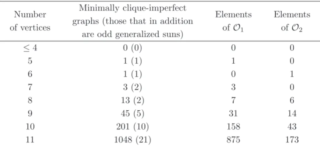
In Table 1 the number of minimally clique-imperfect graphs in the classes O1and O2were tabulated by computer, and suggest that the class O1is much
larger than the class O2.
The analogous to Theorem 15 for coordinated graphs was formulated in [12]: Theorem 19 ([12]) Let G be a graph. Then:
1. γc(G) = χ(K(G)).
2. ∆c(G) ≤ ω(K(G)).
Number of vertices
Minimally clique-imperfect graphs (those that in addition
are odd generalized suns)
Elements of O1 Elements of O2 ≤ 4 0 (0) 0 0 5 1 (1) 1 0 6 1 (1) 0 1 7 3 (2) 3 0 8 13 (2) 7 6 9 45 (5) 31 14 10 201 (10) 158 43 11 1048 (21) 875 173
Table 1: Classifying minimally clique-imperfect graphs
As a consequence,
∆c(G) ≤ ω(K(G)) ≤ χ(K(G)) = γc(G) holds for any graph G,
and coordinated graphs are exactly those for which both inequalities are satisfied at equality for each induced subgraph. Again, as a corollary of Theorem 19 we will obtain Corollary 20, which is another variant of Corollary 9 but in terms of χ-goodness. A graph is called χ-good if χ(G) = ω(G). The same property is not required for induced subgraphs, and for this reason χ-goodness is strictly weaker than perfection. Let us call a graph χ(K)-good if its clique graph is χ-good, and define a graph G to be χ(K)-perfect if all its induced subgraphs are χ(K)-good. Equivalently, G is χ(K)-perfect if and only if χ(K(G′)) = ω(K(G′))
for each induced subgraph G′ of G. Again, the graph of Figure 6 shows that
χ(K)-perfection is strictly weaker than hereditary K-perfection. Finally, the analogous to Corollary 16 is the following.
Corollary 20 If G is a coordinated graph then G is χ(K)-perfect. Furthermore,
if G is hereditary clique-Helly then the converse also holds.
Therefore χ(K)-perfect graphs constitute a superclass of both coordinated graphs and hereditary K-perfect graphs. In [12] the following is proved for coordinated graphs:
Theorem 21 ([12]) If G is a coordinated graph then G has no odd holes and
has no antiholes with more than 6 vertices.
The analogous for hereditary K-perfect graphs was proved in Lemma 3. In the next theorem we extend both results to the class of χ(K)-perfect graphs.
Theorem 22 If G is χ(K)-perfect then G has no odd holes and has no antiholes
with more than 6 vertices.
Proof. Since K(Cn) = Cn then odd holes are not χ(K)-good. In [12] it is shown
that χ(K(Cn)) ≥ (|V (K(Cn))| − 1)/2 for each n ≥ 5 and a recursive formula is
given for |V (K(Cn))| which implies that |V (K(Cn))| > 2n + 1 for n ≥ 8. All
along the proof, Cnwill denote the graph such that V (Cn) = {0, 1, . . . , n−1} and
E(Cn) = {01, 12, 23, . . . , (n − 1)0}. Let Q be a clique of Cn and define the orbit
of Q as O(Q) = {Q + j : 0 ≤ j ≤ n − 1} where Q + j stands for {a + j : a ∈ Q}
and the sum is taken modulo n. The period of Q is |O(Q)|. The orbits induce a partition of the cliques of Cn and the period of each clique Q divides n. For
each clique Q of Cnit holds that (Q + j) ∩ (Q + j + 1) = ∅ and consequently any
complete of K(Cn) cannot contain both Q+j and Q+j +1 for any j. Therefore,
each complete of K(Cn) contains at most ⌊|O(Q)|/2⌋ members of O(Q), for each
clique Q of Cn (where ⌊x⌋ denotes the largest integer not exceeding x).
Since K(C7) = C7 then C7 is not χ(K)-good, so henceforth we can assume
that n ≥ 8. We claim that there is a set S that is the union of orbits of cliques of Cn such that any complete of K(Cn) contains at most |S|/2 − 1 elements of
S. This will imply that ω(K(Cn)) ≤ (|V (K(Cn))| − 2)/2, which together with
χ(K(Cn)) ≥ (|V (K(Cn))| − 1)/2 shows that Cn is not χ(K)-good.
When n is odd this is easy. Since we are assuming that n ≥ 8 then |V (K(Cn))| > 2n + 1 and then there are at least two cliques Q1 and Q2 of
Cn such that O(Q1) ∩ O(Q2) = ∅ and let S = O(Q1) ∪ O(Q2). Since n is odd
then |O(Q1)| and |O(Q2)| are both odd and each complete of K(Cn) contains
at most ⌊|O(Q1)|/2⌋ + ⌊|O(Q2)|/2⌋ = (|O(Q1)| + |O(Q1)|)/2 − 1 = |S|/2 − 1
elements from S, and the claim is proved.
Consider the case when n = 4k + 4 and k ≥ 1. Let a1, . . . , a2k+1be the finite
sequence formed by k terms equal to 2, followed by one 3, followed by k − 1 terms equal to 2, followed by one 3, and let Q ⊆ {0, 1, . . . , n − 1} be the set of the partial sums of {ai} modulo n, i.e., Q = {b1, . . . , b2k+1} where biis equal to
a1+ · · · + ai modulo n, for each i = 1, 2, . . . , 2k + 1 (in particular, b2k+1= 0).
Then Q is a clique of Cn of period n. Let S = O(Q) and let Q be any complete
of K(Cn). If Q∩S = ∅ then the claim is trivially true. Without loss of generality
Q ∈ Q. By construction, Q ∩ (Q + 2k + 2) = ∅, thus Q + 2k + 2 /∈ Q. Since Q does not contain both Q + j and Q + j + 1 for any j then Q contains at most 2k + 1 = |S|/2 − 1 elements of S, as claimed.
Finally, consider the case n = 4k + 6 for any k ≥ 1. Let a1, . . . , a2k+2 be
the finite sequence formed by k terms equal to 2, followed by one 3, followed by k terms equal to 2, followed by one 3, let b1, . . . , b2k+2be the sequence formed
by k terms equal to 2, followed by one 3, followed by k − 1 terms equal to 2, followed by one 3, followed by one 2, and let Q1, Q2⊆ {0, 1, . . . , n − 1} be the
partial sums modulo n of {ai} and {bj}, respectively. Then Q1 and Q2 are
cliques of Cn, Q1 has period n/2 = 2k + 3 and Q2 has period n = 4k + 6. Let
S = O(Q1) ∪ O(Q2) and let Q be any complete of K(Cn). It is enough to prove
that |Q ∩ S| ≤ 3k + 3. If Q ∩ O(Q2) = ∅ then the claim is trivially true. Without
|Q ∩ O(Q2)| ≤ 2k + 2. Since necessarily |Q ∩ O(Q1)| ≤ k + 1, we conclude that
|Q ∩ S| ≤ 3k + 3 and the claim is proved also in this case. ¤ We have the following inclusions:
coordinated ⊂ χ(K)-perfect ⊂ ({C2k+1: k ≥ 2} ∪ {Cn : n ≥ 7})-free ⊂ perfect.
To see that the three inclusions are proper, notice that the 3-sun is χ(K)-perfect (as it is hereditary K-χ(K)-perfect) but not coordinated since ∆c(3-sun) = 3
and γc(3-sun) = 4, and that S2 (cf. Figure 10, p. 28) has no odd holes and no
antiholes but K(S2) is not χ-good since ω(K(S2)) = 3 and χ(K(S2)) = 4, and
finally C8proves that the rightmost inclusion is also proper.
As we did with the classes O1 and O2, we propose to classify the minimal
forbidden induced subgraphs for the class of coordinated graphs into two classes of obstructions. The class O3 of those graphs G with ∆c(G) < ω(K(G)) and
the class O4 of those graphs G for which ω(K(G)) < χ(K(G)) holds. Again,
Theorem 19 tells us that hereditary clique-Helly obstructions satisfy ∆c(G) =
ω(K(G)), and necessarily belong to the class O4. The obstructions appearing
in the partial minimal forbidden induced subgraphs characterizations in the literature belong all to the class O4 with the only exceptions of the 3-sun, 2P4
and R (cf. Theorem 34).
Finally, note that the α(K)-perfect and χ(K)-perfect graphs define classes that are incomparable because C9is α(K)-perfect but not χ(K)-perfect, and the
viking with 7 vertices (cf. Figure 10, p. 28) is χ(K)-perfect but not α(K)-perfect. The graph of Figure 6 is α(K)-perfect and χ(K)-perfect but not K-perfect, and proves the following proper inclusion:
hereditary K-perfect ⊂ α(K)-perfect ∩ χ(K)-perfect
5
Partial characterizations
In this section we review characterizations of clique-perfect and coordinated graphs when restricted to different graph classes. We review the previous re-sults, present some new contributions and formulate the main open problems. Computational complexity issues are also discussed.
The class of clique-perfect graphs is hereditary and thus admits some forbid-den induced subgraph characterization. Nevertheless, although some families of forbidden induced subgraphs were identified and some partial characterizations were formulated, a complete list of forbidden induced subgraphs for the class of clique-perfect graphs is not known. Furthermore, the problem of determining the complexity of the recognition of clique-perfect graphs is also open. These two questions are regarded as the main open problems related to clique-perfect graphs (see for instance [10]).
The coordinated graph recognition problem is NP-hard and it is NP-complete even restricted to {gem,C4,odd hole}-free graphs with ∆ = 4, ω = 3 and
complete list of minimal forbidden induced subgraphs. This problem seems to be difficult because in [69] several families of minimally non-coordinated graphs were described whose cardinality grows exponentially on the number of vertices and edges.
Although there are some partial results, the problem of given a characteriza-tion by forbidden induced subgraphs of neighborhood-perfect graphs is also open in general. Similarly, although some polynomial-time algorithms for recogniz-ing neighborhood-perfectness when the input graph is known to belong to cer-tain graph classes, the computational complexity of recognizing neighborhood-perfect graphs in general is not known. These are the main open problems regarding neighborhood-perfect graphs.
In this section we present the known partial results on clique-perfect, co-ordinated graphs, and/or neighborhood-perfect graphs regarding the problems of characterizing by minimal forbidden induced subgraphs and determining the computational complexity of their recognition when restricted to different graph classes. These graph classes are: chordal graphs, diamond-free graphs, P4-tidy
graphs, Helly circular-arc graphs, complements of forests, line graphs and com-plements of line graphs, some other subclasses of claw-free graphs and two su-perclasses of triangle-free graphs.
5.1
Chordal graphs
Lehel and Tuza [53] proved that in chordal graphs, balanced and neighborhood-perfect graphs coincide and they are those graphs with no induced odd suns. This, together with Theorem 17, implies the following result.
Theorem 23 ([53, 9]) Let G be a chordal graph. Then G is clique-perfect if
and only if G contains no induced odd sun, if and only if G is balanced, if and only if G is neighborhood-perfect.
Notice that odd suns may properly contain odd suns as induced subgraphs, thus unfortunately this characterization is not by minimal forbidden induced subgraphs. Indeed, it is an open problem to determine the minimal odd suns in the sense of induced subgraphs. As balanced graphs can be recognized in polynomial time, the same algorithm solves, in polynomial time, the problem of recognizing clique-perfect graphs (and thus neighborhood-perfect graphs) re-stricted to chordal graphs.
Since clique-perfect chordal graphs coincide with balanced chordal graphs then both are subclasses of coordinated chordal graphs. The inclusion is proper since, for instance, the graph displayed in Figure 7 is an example of an odd sun that is coordinated. The fact that clique-perfect chordal graphs are balanced implies, by Theorem 14, that for clique-perfect chordal graphs both parameters αc and τc (that coincide) can be computed in polynomial time.
Notice that also the 3-sun is chordal and hereditary K-perfect but not clique-perfect, or coordinated. So hereditary K-perfection does not coincide with co-ordination or clique-perfection or balancedness even when restricted to chordal graphs.
Figure 7: A chordal coordinated odd sun.
5.2
Diamond-free graphs
The characterization by forbidden induced subgraphs of those diamond-free graphs that are clique-perfect is the following:
Theorem 24 ([11]) Let G be a diamond-free graph. Then G is clique-perfect
if and only if G contains no induced odd generalized sun.
In fact, the authors prove that diamond-free graphs with no odd generalized suns are hereditary Helly and hereditary K-perfect, and therefore clique-perfect.
The problem of deciding whether there exists a polynomial-time algorithm for the recognition of the clique-perfection of a diamond-free graph was left open in [11]. This problem was solved in [15], where it was proved that such an algorithm exists, based on the following result.
Theorem 25 ([15]) Let G be a diamond-free graph. Then G is clique-perfect
if and only if G is balanced.
Proof. Since balanced graphs are clique-perfect then we only need to prove
that diamond-free clique-perfect graphs are balanced, or equivalently, that a diamond-free graph that is not balanced is not clique-perfect. Assume that G is a diamond-free graph and that G is not balanced. By Theorem 6, G contains an unbalanced cycle C, that is, an odd cycle C and for each edge e of C a (possibly empty) complete We ⊆ NG(e) \ C such that NC(We) ∩ NC(e) = ∅.
We claim that C is proper. Suppose, for contradiction, that some edge e = xy of C is improper, and let v in C such that {x, y, v} is a triangle of G. Since NC(We) ∩ NC(e) = ∅, then there is a vertex w ∈ We such that v is not
adja-cent to w, and thus {v, w, x, y} induces a diamond in G, a contradiction. We conclude that C is proper and thus V (C) induces an odd generalized sun. By Theorem 17, G is clique-imperfect. ¤ Thus, the problems of recognizing balancedness and recognizing clique-per-fection coincide when restricted to diamond-free graphs. Therefore the recogni-tion of clique-perfecrecogni-tion can also be solved in polynomial time for diamond-free graphs. Moreover, by Theorems 14 and 25, αc (and therefore also τc) can be
Figure 8: A coordinated diamond-free odd generalized sun.
Notice that if G is a diamond-free graph, the problem of deciding whether G is a minimal odd generalized sun can be solved in polynomial time (it suffices to check that G is not clique-perfect but G − {v} is clique-perfect for every vertex v of G). Surprisingly, the problem of deciding whether G is an odd generalized sun (not necessarily minimal) is NP-complete even if G is a triangle-free graph [50]. Notice that an odd cycle in a triangle-triangle-free graph cannot have improper edges. Hence, if G is a triangle-free graph with an odd number of vertices, then G is an odd generalized sun if and only if G has a Hamiltonian cycle, and the Hamiltonian cycle problem on triangle-free graphs with an odd number of vertices is NP-complete [43, pp. 56–60].
Since
balanced graphs ⊂ hereditary clique-Helly∩hereditary K-perfect ⊂ clique-perfect holds and diamond-free graphs are hereditary clique-Helly we conclude, as a corollary of Theorem 25 and its proof, the following.
Corollary 26 Let G be a diamond-free graph. Then the following conditions
are equivalent (and can be decided in polynomial time): 1. G is balanced.
2. G is hereditary K-perfect. 3. G is clique-perfect.
4. G contains no induced proper odd cycle.
Since diamond-free clique-perfect graphs are balanced then they are also coordinated. Therefore the class of clique-perfect diamond-free graphs is a sub-class of the sub-class of coordinated diamond-free graphs. The inclusion is proper since the graph of Figure 8 is coordinated but not clique-perfect.
Odd holes and complete odd suns are minimally clique-imperfect. However, there are other odd generalized suns that contain proper induced odd generalized suns and consequently are not minimally clique-imperfect. The same is true even for proper odd cycles. Thus, the characterizations of Theorem 25 and Corollary 26 are not by minimal forbidden induced subgraphs. The minimal forbidden induced subgraph characterization of clique-perfect (or equivalently balanced) graphs restricted to diamond-free graphs was described in [1]. The corresponding minimal forbidden diamond-free induced subgraphs are the odd holes and the sunoids (which can be put in correspondence with Dyck-paths); the reader is referred to [1] for the details.
5.3
Superclasses of cographs
It is known that comparability graphs are clique-perfect [2]. Since cographs are comparability graphs [42] then cographs are also clique-perfect. In [51] the authors gave a simpler proof of the clique-perfection of cographs based on the following result.
Theorem 27 ([51]) Let G be the join of the graphs G1 and G2. Then αc(G) =
min{αc(G1), αc(G2)} and τc(G) = min{τc(G1), τc(G2)}. In particular, G is
clique-perfect if and only if G1 and G2 are clique-perfect.
As a corollary it is possible to compute αc(G) and τc(G) of a given cograph G
in linear time by first computing its cotree [29].
Distance-hereditary graphs and P4-tidy graphs define two superclasses of
cographs not included in the class of comparability graphs. In [52], distance-hereditary graphs were shown to be clique-perfect, relying on a decomposition tree of distance-hereditary graphs introduced in [21]. In [52], linear-time al-gorithms for computing αc(G) and τc(G) for any distance-hereditary graph are
also presented. In [15], those P4-tidy graphs that are clique-perfect were
charac-terized by minimal forbidden induced subgraphs. Moreover, it was shown that the problems of recognizing clique-perfect graphs can be solved in linear time for P4-tidy graphs.
Theorem 28 ([15]) Let G be a P4-tidy graph. Then G is clique-perfect if and
only if G contains neither C5 nor 3-sun as an induced subgraph. Moreover,
clique-perfectness of P4-tidy graphs can be decided in linear time.
Furthermore, it was shown that both parameters that define clique-perfect-ness can be computed in linear time for P4-tidy graphs.
Theorem 29 ([15]) There are linear-time algorithms that compute αc(G) and
τc(G) for any given P4-tidy graph G.
The proof of the above theorems relies on the structural characterization of P4-tidy graphs given in Theorem 5. Analogous results to the above theorems
for neighborhood-perfectness of P4-tidy graphs were obtained in [37].
Theorem 30 ([37]) A P4-tidy graph G is neighborhood-perfect if and only if
G has no induced 3K2, 3-sun, or C5. Moreover, neighborhood-perfectness of
P4-tidy graphs can be decided in linear time.
Theorem 31 ([37]) There are linear-time algorithms that compute αn(G) and
ρn(G) for any given P4-tidy graph G.
Since the 3-sun and C5 are not coordinated, the class of coordinated P4
-tidy graphs is included in the class of clique-perfect P4-tidy graphs. Moreover,
the inclusion is proper since the graph tent ∪ K2 is P4-tidy and clique-perfect
Figure 9: The graph R
3K2 is an example of a coordinated P4-tidy graph that is not
neighborhood-perfect; thus, coordinated P4-tidy graphs are not contained in
neighborhood-perfect P4-tidy graphs.
It was proved in [9] that if F is a forest then F is clique-perfect. As the class of complements of forests is closed under taking induced subgraphs, it suffices to prove that αc(F ) = τc(F ). We may assume that F has no isolated vertex,
because if u were an isolated vertex of F then every clique of F would contain u implying αc(F ) = τc(F ) = 1. Thus F has no universal vertex, which means
that τc(F ) > 1. Moreover F has some leaf u and let v be the only neighbor of
u in F . Then {u, w} is a clique-transversal of F , which shows that τc(F ) = 2.
Furthermore, since every connected component of F is a tree with at least two vertices, αc(F ) = τc(F ) = 2. This, together with Theorem 27 immediately
implies the following.
Theorem 32 ([9, 51]) Every tree-cograph is clique-perfect.
In [37], the following characterization of neighborhood-perfect graphs by forbidden induced subgraphs was proved.
Theorem 33 ([37]) If G is a tree-cograph, then G is neighborhood-perfect if
and only if G contains no induced 3K2 or P6+ 3K1.
Moreover, from this a linear-time recognition algorithm for neighborhood-perfectness of tree-cographs was also found in [37]. Furthermore, in the same work, linear-time algorithms for computing αn(G) and ρn(G) for any
tree-cograph G were devised. In the following subsection, we will present the char-acterization of coordinated graphs for complements of forests, a subclass of tree-cographs.
5.4
Complements of forests
Recall from the previous subsection that all complements of forests are clique-perfect. Moreover, it follows from Theorem 33 that those complements of forests that are neighborhood-perfect are those that are 3-pyramid-free. In [18] a characterization by minimal forbidden induced subgraphs of those coordi-nated graphs within the class of complements of forests was found. Recall that 2P4 is the disjoint union of two P4’s and let R be the graph depicted in
Fig-ure 9. Both 2P4 and R are not coordinated, since ∆c(2P4) = ∆c(R) = 6 and
γc(2P4) = γc(R) = 7. The characterization is as follows.
Theorem 34 ([18]) Let G be the complement of a forest. Then G is
A characterization of those forests obtained by identifying the false twins of G when G is coordinated, called c-forest, leads to a linear time recognition algorithm for coordinated graphs within the class of complements of forests [18].
5.5
Line graphs and complements of line graphs
The characterization by forbidden induced subgraphs of those line graphs that are clique-perfect is as follows.
Theorem 35 ([10]) Let G be a line graph. Then G is clique-perfect if and only
if G has no odd holes and contains no induced 3-sun.
The first part of the proof consists of proving that perfect line graphs are K-perfect, and relies on the characterization of perfect line graphs in [58] and on a property of clique-cutsets in perfect graphs [5]. Therefore, those perfect line graphs that are in addition hereditary clique-Helly are also clique-perfect. In the second part of the proof those line graphs that are not hereditary clique-Helly are treated separately. In fact, hereditary K-perfection and clique-perfection do not coincide for line graphs as one realizes by considering the 3-sun.
Those line graphs that are coordinated were characterized by forbidden in-duced subgraphs in [18].
Theorem 36 ([18]) Let G be a line graph. Then G is coordinated if and only
if G has no odd hole and contains no induced 3-sun.
Reasoning as in the first part of the proof of Theorem 35, line graphs without odd holes are K-perfect, and then those that in addition are hereditary clique-Helly, are coordinated. Therefore the proof consists of studying those line graphs that have no odd holes but have some family of cliques that does not satisfy the Helly property.
Notice that by Theorems 35 and 36, coordinated and clique-perfect graphs coincide when restricted to line graphs.
In [18] also a characterization of coordinated line graphs in terms of its root graph is given. To formulate it, the authors introduce the following definitions. Given a graph H and a set S ⊆ V (H), denote by EH(S) the set of edges of H
that have both endpoints in S. The set S ⊆ V (H) is an edge separator of H if every vertex of S belongs to a different connected component of G \ EH(S).
Let t = {v1, v2, v3} be a triangle of a graph H. The triple (v1, v2, v3) is a well
ordering of t if dH(v1) ≤ dH(v2) ≤ dH(v3) and at least one of the following
conditions holds: (i ) dH(v1) < dH(v2), or (ii ) NH[v3] is equal to both NH[v1]
and NH[v2], or (iii ) NH[v3] is equal to none of NH[v1] and NH[v2]. Every
triangle admits some well ordering permutation [18]. Let Etbe the set of edges
{v1v2, v2v3, v3v1}, and if T is a family of triangles, let ET =St∈T Et. With
this terminology, the characterization can now be formulated as follows: Theorem 37 ([18]) Let H be a graph and T be the set of triangles of H. Then
1. L(H) is coordinated.
2. H \ET is bipartite and every well ordered triangle (v1, v2, v3) of H satisfies
one of the following statements:
(a) dH(v1) = 2 and NH[v2] ∩ NH[v3] is an edge separator of H.
(b) dH(v1) = 3, v1 and v2are true twins and NH[v1] is an edge separator
of G.
This characterization leads to a linear-time recognition algorithm for coor-dinated graphs within the class of line graphs. As a corollary, a linear-time recognition algorithm for clique-perfect graphs within this class follows. In [18], a linear-time algorithm for determining ∆c(G) and γc(G) for any coordinated
line graph G = L(H) is also presented.
We would like to remark that the first part of the proof of Theorem 36 implies the following: a line graph is hereditary K-perfect if and only if it has no odd holes, if and only if it is perfect.
In [16], clique-perfectness of complements of line graphs was characterized by minimal forbidden induced subgraphs.
Theorem 38 ([16]) If G is the complement of a line graph, then G is
clique-perfect if and only if G contains no induced 3-sun and has no antihole Ck for
any k ≥ 5 such that k is not a multiple of 3.
Let G be the complement of the line graph of a graph H. In order to prove the above theorem, the parameters αc(G) and τc(G) are expressed in terms of
the graph H. Clearly, the cliques of G are precisely the maximal matchings of H. The matching-transversal number of H, denoted by τm(H), is defined as
the minimum size of a set of edges of H that meets every maximal matching of H. Similarly, the matching-independence number of H, denoted by αm(H),
is defined as the maximum size of a set of pairwise-disjoint maximal matchings of H. A graph is called matching-perfect [16] if τm(H) = αm(H) for every
subgraph (induced or not) of H. It is not hard to see that G is clique-perfect if and only if H is matching-perfect. In fact, the proof of Theorem 38 follows as a corollary of the following characterization of matching-perfect graphs. Theorem 39 ([16]) A graph H is matching-perfect if and only if H contains
no bipartite claw and the length of each cycle of H is at most 4 or a multiple of
3.
In its turn, Theorem 39 is proved by means of a decomposition theorem describing in detail the linear and circular structure of graphs containing no bipartite claw proved in [16].
Notice that since the 3-sun and antiholes different from C6 are neither
co-ordinated nor neighborhood-perfect, coco-ordinated (resp. neighborhood-perfect) complements of line graphs are clique-perfect. Moreover, these inclusion are proper and coordination and neighborhood-perfectness differ for complements of line graphs. In fact, the 3-pyramid = L(K4) is clique-perfect and
coordi-nated but not neighborhood-perfect, whereas 2P4 = L(2P5) is clique-perfect
Figure 10: Minimal forbidden induced subgraphs for clique-perfect graphs inside the class of Helly circular-arc graphs. Dashed lines represent induced paths of length 2k − 3 for each k ≥ 2.
5.6
Helly circular-arc graphs
In [11] a characterization of those Helly circular-arc graphs that are clique-perfect was formulated in terms of forbidden induced subgraphs. The forbidden induced subgraphs are displayed in Figure 10. The 3-sun, odd holes, vikings and 2-vikings are all odd generalized suns. The authors show that, within Helly circular-arc graphs, there are only two families of minimally clique-imperfect graphs which are not odd generalized suns or antiholes, namely, Sk and Tk for
each k ≥ 2. Since the graphs of Figure 10 do not contain properly each other as induced subgraphs then the following is a characterization by minimal forbidden induced subgraphs:
Theorem 40 ([11]) Let G be a Helly circular-arc graph. Then G is
clique-perfect if and only if it does not contain a 3-sun, an antihole of length 7, an odd hole, a viking, a 2-viking or one of the graphs Sk or Tk for each k ≥ 2.
Whether a graph is a Helly circular-arc graph can be decided in linear time and, if affirmative, both parameters αc(G) and τc(G) can also be computed in
linear time [34, 35, 55]. However, these facts do not immediately imply the existence of a polynomial-time recognition algorithm for clique-perfect Helly circular-arc graphs (because we need to verify the equality for every induced subgraph). The characterization given in [11] leads to such an algorithm, which is strongly based on the recognition of perfect graphs [23]. The idea of the algorithm is similar to the one used in [28] for recognizing balanceable matri-ces. It was proved in [75] that clique-perfectness coincides with neighborhood-perfectness for Helly circular-arc graphs. As in [11], the proof strategy consists in studying separately those Helly circular-arc graphs that are hereditary clique-Helly from those that are not so.
Theorem 41 ([75]) If G is a Helly circular-arc graph, then G is clique-perfect